Abstract

A five-dimensional lattice space is decomposed into a number of four-dimensional lattices called ‘layers’. We can interpret the five-dimensional gauge theory as four-dimensional gauge theories on the multi-layer with interactions between neighboring layers. In the theory, there exist two independent coupling constants: $\beta_{4}$ controls the dynamics inside a layer, and $\beta_{5}$ does the strength of the inter-layer interaction. We propose the new possibility to realize the continuum limit of a five-dimensional theory using four-dimensional dynamics with large $\beta_{4}$ and small $\beta_{5}$. Our result is also related to the higher dimensional theory by deconstruction approach.

PACS number(s): 11.10.Kk, 11.15.Ha, 11.25.Mj

1 Introduction

Kaluza and Klein (KK)’s idea was a nice unification scenario that a four-dimensional gravity and a Maxwell theory are derived from a five-dimensional gravity[1]. But their approach was done within a classical framework and it is not so easy to realize its quantum theory. The first problem is that five-dimensional theories are generally unrenormalizable even if they are renormalizable theories in four dimensions. The another point is that the property of phase transitions in five-dimensional lattice theories is exactly same as that of mean-field theories. The latter implies that it is generally difficult to take the continuum limit in the five-dimensional theory using the second order phase transition and the associated fixed point (FP). Actually, some searches for both properties in a five-dimensional gauge theory have been tried [2, 3, 4, 5] and it is still far that one realizes a continuum limit from five-dimensional statistical mechanics.

Although most of possibilities in the construction of five-dimensional theories are shut, there is a path to the construction, that is to use well-known properties of a four-dimensional statistical mechanics. Since we know the continuum limit of a four-dimensional gauge theory, the limiting operation keeping fixed physical quantities can be considered in the meaning of a four-dimensional theory. Recently, a new approach for the KK’s scenario called deconstruction has appeared using four-dimensional asymptotically free gauge theories in the continuum[6, 7]. The approach realizes KK-like modes although they are completely four-dimensional theories. It is an interesting idea but can not give any answer for difficulties of higher dimensional theories because the idea is based on the perturbative picture of four-dimensional theories and has nothing to any clue about properties of the statistical mechanics.

On the other hand, Fu and Nielsen suggested to reduce the extra-dimensional space by the dynamics of a higher-dimensional lattice gauge theory[8]. In the idea, they considered a decomposition of a five-dimensional lattice space into an ensemble of four-dimensional lattice spaces (multi-layer). Unfortunately, they studied about compact $U(1)$ gauge theories which have no continuum limit in four dimensions[9, 10, 11, 12]. In this paper, we formulate a five-dimensional lattice $SU(2)$ gauge theory as a block of four-dimensional theories with an extra interaction like as Fu and Nielsen. The phase structure of the theory is clarified with Monte Carlo simulation and we discuss about the continuum limit as a four-dimensional multi-layer system (multi-layer world). Finally, we suggest how to construct a five-dimensional theory by explicit limiting operations. A limiting curve corresponding to five-dimensional scale shall becomes to an envelope.

The outline of our paper is as follows: our model setting and the notation are explained in the next section. In sec.3, our model is investigated by a numerical method. In sec.4, we discuss physical properties of our model such as gauge squared mass matrix, the four-dimensional continuum limit and suggestion of a new idea for defining a five-dimensional theory. Sec.5 is devoted to summary and discussions.

2 Our Model

In this section, we shall set our model in addition to explanation for a layer structure in the five-dimensional lattice. Link variables along a fifth direction are interpreted as scalar fields in the model. Naively, this has a picture of a four-dimensional theory in the continuum limit. Afterwards, measured order parameters in our numerical simulation are listed and an expected phase diagram is sketched.

1. Layer structure and Wilson action We consider the five-dimensional pure $SU(2)$ Wilson action on a $N_{4}^{4}\times N_{5}$ lattice with a periodic boundary condition:

$$S_{\rm lat} = \beta_{4}\sum_{P_{4}}\left[1-\frac{1}{2}{\rm~{}Tr}\,U_{P_{4}}\right]+\beta_{5}\sum_{P_{5}}\left[1-\frac{1}{2}{\rm~{}Tr}\,U_{P_{5}}\right]\ ,$$ (1)

$${\rm~{}Tr}\,U_{P_{4}} \equiv {\rm~{}Tr}\,U_{n,\mu}^{n_{5}}\ U_{n+\hat{\mu},\nu}^{n_{5}}\ U_{n+\hat{\nu},\mu}^{\dagger n_{5}}\ U_{n,\nu}^{\dagger n_{5}}\ ,$$ (2)

$${\rm~{}Tr}\,U_{P_{5}} \equiv {\rm~{}Tr}\,U_{n,\mu}^{n_{5}}\ U_{n+\hat{\mu},5}^{n_{5}}\ U_{n,\mu}^{\dagger n_{5}+1}\ U_{n,5}^{\dagger n_{5}}\ ,$$ (3)

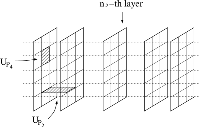
where the sum is defined as $\sum_{P_{4}}\equiv\sum_{n,n_{5}}\ \sum_{1\leq\mu<\nu\leq 4}\ ,\ \sum_{P_{5}}\equiv\sum_{n,n_{5}}\ \sum_{1\leq\mu\leq 4}$ . According to Fu and Nielsen[8], we call the four-dimensional subspace a ‘layer’, because the individual four-dimensional subspace must be independent of each other if $\beta_{5}$ is equal to zero. Every layer was aligned along the fifth direction $-\!\!\!-$ see Fig.1. An $n_{5}$-th layer is noted ${\cal L}_{n_{5}}$. $U_{n,\mu}^{n_{5}}$ is a link variable inside ${\cal L}_{n_{5}}$ and $U_{n,5}^{n_{5}}$ connects between ${\cal L}_{n_{5}}$ and ${\cal L}_{n_{5}+1}$. These link variables behave as $\underline{2}$ of $SU(2)$. Then the first term of the action (1) represents interactions inside layers controlled by $\beta_{4}$, and the second term represents interactions between different layers (inter-layer) controlled by $\beta_{5}$. Note that for convenience two coupling constants,

$$\beta\equiv\sqrt{\beta_{4}\beta_{5}}\ ,\ \gamma\equiv\sqrt{\frac{\beta_{5}}{\beta_{4}}}\ ,$$ (4)

are also used.

2. Measuring quantities To understand the dynamics of (1), the following quantities are measured.

• Expectation values of the plaquette $U_{P_{4}}$ inside a layer and $U_{P_{5}}$ between neighboring layers.

• Creutz ratio of loops inside a layer,

  $$\sigma_{4}(l_{\mu},l_{\nu})\equiv-{\rm ln}\left\{\frac{W(l_{\mu},l_{\nu})W(l_{\mu}-1,l_{\nu}-1)}{W(l_{\mu},l_{\nu}-1)W(l_{\mu}-1,l_{\nu})}\right\}\ ,$$ (5)

  where $W(l_{\mu},l_{\nu})$ implies an expectation value of Wilson loop with $l_{\mu}\times l_{\nu}$ size on the same layer.

• Polyakov loop along fifth direction,

  $$L_{5,n}\equiv\frac{1}{2}{\rm Tr}\prod_{n_{5}}U_{n,5}^{(n_{5})}\ .$$ (6)

• Inverse of correlation length for Polyakov loops,

  $$\left<L_{5,n}L_{5,m}\right>-\left<L_{5,n}\right>^{2} \sim \cosh(-H\left|n-m\right|)\ .$$ (7)

$U_{P_{4}}$ and $U_{P_{5}}$ correspond to parts of the internal energy. $\sigma_{4}(l_{\mu},l_{\nu})$ is an order parameter of four-dimensional confinement inside a layer and $\left<L_{5,n}\right>$ is that of $Z_{2}$ center symmetry .

3. Intuitive understanding of dynamics Depending on the magnitude of $\beta_{4},\beta_{5}$, the dynamics (1) has various feature. In the case that $\gamma$ is larger than unity, inter-layer interactions are strong compared to those inside layers. In this region the influence among the layer can not be ignored because a layer is strongly bound to its neighboring layers. It seems difficult to control the system in taking the continuum limit because there remain the strong extra-interactions caused by the fifth direction in the coupling region. As $\gamma$ is smaller than unity, interactions of inter-layer are weaker than those of inside layers. Then layers are loosely bound to each other, and in this region the dynamics is similar to a four-dimensional gauge theory with extra fields. We call this picture a ‘multi-layer world’.

From two order parameters $\sigma_{4}$ and $\left<L_{5}\right>$ we can imagine four phases. Since our model is reduced to a four-dimensional gauge theory at $\beta_{5}=0$, we know that the phase of $\sigma_{4}=0$ and $\left<L_{5}\right>=0$ is not realized $-\!\!\!-$ see Fig.2.

4. Naive continuum limit as four-dimensional gauge theory We consider the naive continuum limit of our model for a particular case which $U_{n,5}^{n_{5}}$ is interpreted as a fundamental ‘scalar’ field $V^{n5}_{n}$ on the ${\cal L}_{n_{5}}$. In the interpretation, the fifth direction is simply an internal degree of freedom. We should consider limit $a_{4}\rightarrow 0$ as the naive continuum limit because there is only lattice spacing $a_{4}$ inside layers. In the first term of the action (1) $\Sigma_{n_{5}}$ corresponds to a trace operation in the internal space and $\Sigma_{n}$ dose to the summation of four-dimensional space. Then the relation between the inside layer coupling $\beta_{4}$ and a four-dimensional gauge coupling $g_{4}$ is determined as

$$\beta_{4}=\frac{4}{g_{4}^{2}}\ .$$ (8)

On the other hand, the second term of the action (1) means interactions between gauge field and ‘scalar’ field written as

$$U_{P_{5}} = U_{n,\mu}^{n_{5}}\ V_{n+\hat{\mu}}^{n_{5}}\ U_{n,\mu}^{\dagger n_{5}+1}\ V_{n}^{\dagger n_{5}}\ .$$ (9)

The $\beta_{5}$ is the inter-layer coupling which controls dynamics of ‘scalar’ fields, and it is determined from the renormarization factor in the continuum limit.

3 Numerical Analysis $-\!\!\!\!-\!\!\!\!-$ Phase Structures on Various ${N_{5}}$ $-\!\!\!\!-\!\!\!\!-$

In this section, we investigate the phase structure of our model by using Monte Carlo simulation. We simulate for Wilson action (1) using $N_{4}^{4}\times N_{5}$ lattice ($N_{4}=8,10,12$, $N_{5}=1,2,3,5,6,8$) by heat-bath algorithm. We measure expectation values of plaquettes $\left<U_{P_{4}}\right>$, $\left<U_{P_{5}}\right>$, specific heats $C_{4}\equiv\left<U_{\rm P_{4}}^{2}\right>-\left<U_{\rm P_{4}}\right>^{2}$, $C_{5}\equiv\left<U_{\rm P_{5}}^{2}\right>-\left<U_{\rm P_{5}}\right>^{2}$, Creutz ratio and Polyakov loop with its fluctuation $\chi_{5}\equiv\left<L_{5}^{2}\right>-\left<L_{5}\right>^{2}$. The statistical errors of these measurements are estimated by the jackknife method. In the following figures, open and filled symbols are noted as results of ordered and disordered start respectively. We describe $N_{5}=1$ and $N_{5}>1$ cases separately.

3.1 Case of ${N_{5}=1}$

Fig.3 represents the phase diagram at $N_{5}=1$ and plots measured lines where (i) $\beta_{4}=0$, (ii) $\gamma=1/\sqrt{12}\sim 0.29$, (iii) $\beta_{4}=10.0$ and (iv) $\beta_{5}=10.0$. Our calculations support the expected phase diagram (Fig.2), and their detailed discussions are summarized as follows:

(i) ${\it\beta_{4}=0}$: Fig.4 shows results of $\left<L_{5}\right>$ and $\chi_{5}$. Those quantities imply that the confinement-deconfinement phase transition occurs at $\beta_{5c}\sim 0.6$. Especially in $\chi_{5}$, we can see the volume effect which is a characteristic signal of the phase transition.

(ii) ${\it\beta_{4}=10.0}$: From $\left<L_{5}\right>$, the similar signal of the transition can be seen at $\beta_{5}\sim 0.6$. In addition, $\sigma_{4}$ also bends sharply at $\beta_{5}\sim 0.6$ $-\!\!\!-$ see Fig.5.

(iii) ${\it\beta_{5}=0.3}$: In Fig.6, we can confirm that signal of crossover about $\sigma_{4}$ is exactly same as that of an ordinary four-dimensional lattice gauge theory ($\beta_{5}=0$).

(iv) ${\it\beta_{5}=10.0}$: We can see that $\sigma_{4}$ is decreasing as $\beta_{4}$ is growing in Fig.7, although it is difficult to recognize a rapid change of $\sigma_{4}$ at $\beta_{4}\sim 1.2$.

The naive continuum limit of an $N_{5}=1$ system corresponds to the four-dimensional gauged non-linear $\sigma$ model:

$$S_{\rm lat}\rightarrow\int d^{4}x\left\{\frac{1}{4}{\rm~{}Tr}\,F_{\mu\nu}^{2}+\frac{1}{2}f_{\pi}^{2}\Bigl{(}D_{\mu}V(x)\Bigr{)}^{\dagger}\Bigl{(}D_{\mu}V(x)\Bigr{)}\right\}$$ (10)

where $V(x)$ is a scalar field with a constraint condition

$$V(x)=\theta_{0}(x)+i\vec{\sigma}\cdot\vec{\theta}(x)\ ,$$

$$\quad\theta_{0}^{2}+\vec{\theta}^{2}=1\ .$$ (11)

This condition reads to $(\partial_{\mu}\theta_{0})^{2}\ll(\partial_{\mu}\theta^{a})^{2}$ at $\theta^{a}\ll 1$. Then the system corresponds to a Georgi-Glashow model with a Higgs triplet [14, 15, 16] which is equivalent to a four-dimensional $O(3)$ Heisenberg model.

3.2 Case of ${N_{5}>1}$

The phase diagram for $N_{5}>1$ and measuring directions are shown in Fig.8. Dashed lines are (i) $\gamma=\sqrt{2}$, (ii) $\gamma=0.5,~{}1/\sqrt{2}~{}(\sim 0.71),~{}1/1.2~{}(\sim 0.83)$, (iii) $\gamma=0.29$ and (iv) $\beta_{4}=8.0,~{}10.0$ and $20.0$ respectively.

(i) ${\it\gamma=\sqrt{2}}$: In Fig.9, as $\beta$ becomes to large, the new phase appears at $\beta\sim 1.2$ where the phase varies from $\sigma_{4}\neq 0$ and $\left<L_{5}\right>=0$ to $\sigma_{4}\neq 0$ and $\left<L_{5}\right>\neq 0$. Afterward the new phase transition occurs at $\beta\sim 2.0$ where the phase varies from $\sigma_{4}\neq 0$ and $\left<L_{5}\right>\neq 0$ to $\sigma_{4}=0$ and $\left<L_{5}\right>\neq 0$.

(ii-a) ${\it 0.5\leq\gamma\leq 0.83}$: In the middle range of $\gamma$, we found a first order phase transition for both order parameters $U_{P_{4}}$ and $U_{P_{5}}$ on a $8^{4}\times 2$ lattice in Fig.10. There the hysteresis loop is clearly seen at $\gamma=0.71$. As $N_{5}$ approaches to $N_{4}$, the range is wider and includes unity where the theory is recovered as usual five-dimensional one. Then this signal of the first order transition corresponds to that of the isotropic five-dimensional $SU(2)$ gauge theory [3].

(ii-b) ${\it 0.0\leq\beta_{5}\leq 1.2}$: Fig.11 shows a change of $\sigma_{4}(2,2)$ for $\beta_{4}$. To compare with it, the result of an ordinary four-dimensional lattice is also shown at the circle symbol. As $\beta_{5}$ is larger, a slope of $\sigma_{4}(2,2)$ is deeper. The signal of crossover is changed to the second order phase transition at $\beta_{5}\sim 1.0$ and further the first order phase transition at $\beta_{5}\sim 1.2$. The change of $\sigma_{4}(2,2)$ for $\beta_{5}$ at $\beta_{4}=2.3$, is shown in Fig.12. We can see that $\sigma_{4}(2,2)$ or the tension is slightly varied in small $\beta_{5}$, although it becomes clear in $\beta_{5}>0.8$ near the phase transition.

(iii) ${\it\gamma=0.29}$: We can find the phase transition at $\beta\sim 2.3$ ($\beta_{4}\sim 0.79,\beta_{5}\sim 0.67$). It is a surprising fact in a multi-layer world that the transition point is independent of $N_{5}>1$. Fig.13 shows results of $U_{P_{5}}$ and $C_{5}$ on a $8^{4}\times N_{5}$ lattice, where $N_{5}=1,2,3,5,6$ and $8$. Both quantities for $N_{5}>1$ are unchanged.

(iv) ${\it\beta_{4}=8.0,10.0}$ and ${\it 20.0}$: At $\beta_{4}=10.0$ we can see that the phase transition occurs at $\beta_{5}\sim 0.63$ from $\sigma_{4}\neq 0$ and $\left<L_{5}\right>=0$ to $\sigma_{4}=0$ and $\left<L_{5}\right>\neq 0$ $-\!\!\!-$ see Fig.14. The hysteresis loop can not be seen in their signals. Therefore we expect the phase transition is second order. The inverse correlation length for Polyakov loops shows at $\beta_{4}=10.0$ on a $12^{4}\times 3$ lattice in Fig.15 and also supports the property of the phase transition. In addition, we found that the transition point for $N_{5}>1$ is closer to that for $N_{5}=1$ as $\beta_{4}$ is larger $-\!\!\!-$ see Fig.16.

Those interesting phenomenon in the multi-layer world shall support our discussions in the next section.

4 Multi-Layer World

4.1 Multi-layer world and gauge fields

In this section, we investigate a multi-layer world ($\gamma$ is sufficiently small to unity and $N_{5}>1$). This world is composed of four-dimensional gauge theories bound by ‘scalar’ fields: $V_{n}^{i}\equiv U_{n,5}^{i}$. The fields are transformed as bi-fundamental representations of ${\cal L}_{i}$ and ${\cal L}_{i+1}$. The gauge transformations are defined as

$$U_{n,\mu}^{i} \rightarrow Y^{i}(n)\ U_{n,\mu}^{i}\ {Y^{i}}^{\dagger}(n+\hat{\mu})\hskip 11.38092pt\mbox{for a gauge field inside a ${\cal L}_{i}$, }$$ (12)

$$V_{n}^{i} \rightarrow Y^{i}(n)\ V_{n}^{i}\ {Y^{i+1}}^{\dagger}(n)\hskip 28.45274pt\mbox{for a `scalar' field between ${\cal L}_{i}$ and ${\cal L}_{i+1}$, }$$ (13)

where $Y^{i}(n)$ is an arbitrary element of $SU(2)$. From (13), $V_{n}^{i}$ can be fixed to unity except for $V_{n}^{1}$,

$$\left\{\begin{array}[]{lclll}V_{n}^{1^{\prime}}&=&Y^{1}(n)\ V_{n}^{1}\ {Y^{2}}^{\dagger}(n)&=1\ ,&\\ V_{n}^{2^{\prime}}&=&Y^{2}(n)\ V_{n}^{2}\ {Y^{3}}^{\dagger}(n)&=1\ ,&\\ &\vdots&\\ V_{n}^{N_{5}^{\prime}}&=&Y^{N_{5}}(n)\ V_{n}^{N_{5}}\ {Y^{1}}^{\dagger}(n)&=Y^{1}(n)\left\{\prod_{i=1}^{N_{5}}V_{n}^{i}\right\}{Y^{1}}^{\dagger}(n)&\equiv Y^{1}(n)X_{n}{Y^{1}}^{\dagger}(n)\ .\end{array}\right.$$ (18)

Note that ${\rm~{}Tr}\,V_{n}^{N_{5}^{\prime}}$ is exactly a Polyakov loop $L_{5,n}$. Since a non-trivial $V_{n}^{i}$ can be moved to every inter-layer, this implies that the system has a translational invariance to the fifth direction. In this point, the multi-layer world is significantly different from a just four-dimensional theory.

Based on this setting of the gauge fixing, we consider mass spectrum of vector fields, $A_{n,\mu}^{a\ i}$. The masses include the effect of fluctuations by layers. We get the following mass term,

($$A_{n,\mu}^{2} \equiv a_{4}^{4}\sum_{n,\mu}\sum_{i,j=1}^{N_{5}}\frac{1}{2}A_{n,\mu}^{a\ i}\ M_{ij}^{2}\ A_{n,\mu}^{a\ j}\ ,$$ term) (19)

where the mass squared matrix is defined as

$$M_{ij}^{2} \equiv \frac{\beta_{5}g_{4}^{2}}{4\ a_{4}^{2}}\left\{\left[\begin{array}[]{ccccc}1&-1&&&\\ -1&2&\ddots&&\\ &\ddots&\ddots&\ddots&\\ &&\ddots&2&-1\\ &&&-1&1\\ \end{array}\right]+L_{5,n}^{2}\left[\begin{array}[]{ccccc}1&&&&-1\\ &0&&0&\\ &&\ddots&&\\ &0&&0&\\ -1&&&&1\\ \end{array}\right]\right\}$$ (30)

$$\equiv \frac{\beta_{5}g_{4}^{2}}{4\ a_{4}^{2}}{\cal M}_{ij}$$ (31)

using $U_{n,\mu}^{i}=\exp\left\{i\ a_{4}\ g_{4}\ \frac{\sigma^{a}}{2}\ A_{n,\mu}^{a\ i}\right\}$ . For the purpose that we go ahead to non-perturbative analysis, the mass may be also non-perturbatively defined by the correlation length between different layers. But the analysis is necessary for a large $N_{5}$ lattice and it is beyond our present computer capacity. Therefore, we take the semi-classical approach such that the mass formula is derived by expanding a field $A_{n,\mu}$ and the mass squared matrix is calculated by Monte Carlo simulation. Under this approximation, $L_{5,n}$ can be replaced with $\left<L_{5}\right>\equiv 1/(2V_{4})\cdot\sum_{n}{\rm~{}Tr}\,X_{n}$, and $V_{4}$ is the four-dimensional volume of a layer. In the case of $\left<L_{5}\right>^{2}=1$, we can easily analyze this matrix ${\cal M}_{ij}$ owing to the periodic boundary condition for the fifth direction [6, 7]. Eigenvalues of this matrix are

$$\lambda_{k} = 4\sin^{2}\frac{\pi k}{N_{5}}\quad,\quad k=0,1,\cdots,N_{5}-1\ ,$$ (32)

and at $k\ll N_{5}$, they are simply written as

$$\lambda_{k}=\left(\frac{2\pi k}{N_{5}}\right)^{2}\ .$$ (33)

It is noted that the values for even $k$ are independent of $\left<L_{5}\right>$. Since it is not so easy to get the values for odd $k$, we numerically calculate them with arbitrary $\left<L_{5}\right>$ which is determined by Monte Carlo simulation. Fig.17 shows plots of eigenvalues $\lambda_{k}$ versus $\left<L_{5}\right>^{2}$ at $N_{5}=3,6$ and $12$.

We see that eigenvalues are doubly degenerate at $\left<L_{5}\right>^{2}=1$. In addition, a noteworthy thing is that the eigenvalues at $\left<L_{5}\right>^{2}=1$ and $N_{5}=n$ are equal to the eigenvalues at $\left<L_{5}\right>=0$ and $N_{5}=n/2$ except for its degeneracy. Our system at $\left<L_{5}\right>^{2}=1$ and $N_{5}=n$ has really the corresponding relation to a circular model at $N_{5}=n$, and a system with $\left<L_{5}\right>=0$ and $N_{5}=n/2$ has a relation to a model with $Z_{2}$ orbifolding [6, 7]. This circumstance means that $S^{1}$ and $S^{1}/Z_{2}$ with respectively different topologies are connected by one parameter $\left<L_{5}\right>$ which corresponds to the energy releasing quarks from a layer. The reason is the existence of ’singular’ gauge transformations such as (18) on lattice theories in contrast to continuum theories. The eigenvalues for even $k$ are topology-independent and mainly used in our following analysis because we do not have a clue to change to the topology although topology changing phenomena is an interesting topics.

4.2 Continuum limit as a four-dimensional gauge theory

In this subsection, we shall consider the continuum limit of four-dimensional gauge theories on layers. Since our fifth direction is identified with just a internal space, we take only the continuum limit $a_{4}\rightarrow 0$ on layers. From $\beta_{4}=4/g_{4}^{2}$, we can express the mass squared matrix as

$$M_{k}^{2}=\frac{\beta_{5}}{\beta_{4}a_{4}^{2}}\lambda_{k}\left(\left<L_{5}(\beta_{4},\beta_{5})\right>,N_{5}\right)=\frac{\gamma^{2}}{a_{4}^{2}}\lambda_{k}(\left<L_{5}(\beta_{4},\beta_{5})\right>,N_{5})\ .$$ (34)

At $k\ll N_{5}$, the simple mass formula

$$M_{k}^{2}=\gamma^{2}\left(\frac{2\pi k}{N_{5}a_{4}}\right)^{2}=\frac{1}{N_{5}}\left(\frac{2\pi\gamma k}{a_{4}}\right)^{2}\ ,$$ (35)

is obtained. In order to take the continuum limit $a_{4}\rightarrow 0$ with a fixed mass (34), a possible method exists;

$$N_{5}{\rm~{}fixed,~{}}\gamma\rightarrow 0{~{}\rm and~{}}\frac{\gamma}{a_{4}}\ {~{}\rm finite~{}}.$$

The approach is realized on $\beta_{4}\rightarrow\infty$ with finite $\beta_{5}$. This theory is defined as four-dimensional asymptotically free one using $\sigma_{4}$ in the confinement phase like a la deconstruction. Actually, the scaling for $\sigma_{4}$ is non-trivial because we have to take care of bi-fundamental fields $V_{n}^{n_{5}}$. Our numerical result shows that the scaling is subtly different from an ordinary four-dimensional theory with $\beta_{5}=0$ $-\!\!\!-$ see Fig.11.

Although we can not use $\sigma_{4}$ in the case of the deconfinement phase, from (7) Higgs mass,

$$m_{h}\equiv\frac{H(\beta_{4},\beta_{5},N_{5})}{a_{4}}\ ,$$ (36)

can be considered instead. This quantity is not yet seen as a good data in statistics in Fig.15. But near $\beta_{5c}$ in both phases, it can be seen as the important scaling parameter

$$H\propto|\beta_{5}-\beta_{5c}|^{\nu}$$ (37)

where $\nu$ is a critical exponent for the correlation length and seems less than unity. It is consistent with second order phase transition at $\beta_{5}=\beta_{5c}\sim 0.6$. The observation is supported by no hysteresis loop and the peak of the specific heat. In this standing point, four-dimensional theories with inter-layer interactions are defined for every $\beta_{5}$ (a multi-layer world).

The phase diagram for $N_{5}>1$ in the multi-layer world is not changed by $N_{5}$ $-\!\!\!-$ see Fig.13. This fact suggests us an extension of a multi-layer theory. If we try to extend this internal space to an real extra dimension, $N_{5}$ must be took to infinity. When $N_{5}$ goes to infinity, $M_{k}$ vanishes from (35). To avoid it, it is necessary for a relation among $\gamma,a_{4}$ and $N_{5}$. If we can introduce a new lattice spacing, $a_{5}\sim a_{4}/\gamma$, our squared mass (35) is written as

$$M_{k}^{2}\sim\left(\frac{2\pi k}{N_{5}a_{5}}\right)^{2}\ .$$ (38)

This relation is exactly a KK mass. Originally, our fifth direction is just an internal space but (38) shows the possibility that the internal space is interpreted as fifth direction. Although the explicit definition for $a_{5}$ is discussed in the following subsection, we note that a relation

$$\left(\frac{a_{4}}{a_{5}}\right)^{2}\sim\frac{\beta_{5}}{\beta_{4}}=\gamma^{2}$$ (39)

implies just that anisotropy of gauge coupling constants corresponds to that of lattice spacings like as finite temperature theories.

4.3 Suggestion for a new definition of five-dimensional gauge theory

In the end of the previous subsection, we saw the possibility of an extra dimension. To construct a continuous extra dimension, we must consider the continuum limit ($a_{5}\rightarrow 0$) combining with another limit $a_{4}\rightarrow 0$. This is a hard parameter-tuning but it becomes possible by the balance between extra-dimensional dynamics and four-dimensional one. In order to set the balance, we can define the quantity from (7), (34) and (37),

$${\cal R}\equiv\frac{M_{k}^{2}}{m_{h}^{2}}=\frac{\beta_{5}\lambda_{2}(N_{5})}{\beta_{4}H^{2}(\beta_{4},\beta_{5},N_{5})}\propto\frac{\beta_{5}}{N_{5}^{2}\beta_{4}|\beta_{5}-\beta_{5c}|^{2\nu}}\ .$$ (40)

If this dimensionless quantity is kept as a nonzero finite value in the limit, it is possible to make both a Higgs mass and KK one of the second excited mode finite.

Let us consider when ${\cal R}$ can be nonzero finite. From the $a_{4}\rightarrow 0$ and (40), we should investigate the region where $\beta_{4}$ is large and $H$ is small ($\beta_{5}\sim\beta_{5c}$). Our numerical study in section 3 suggests to us that the phase structure and the parameter $\beta_{5c}$ unchanged under various $N_{5}>1$. So, we can concentrate on large $\beta_{4}$ and small $H$ independent of $N_{5}$. After of all, we can introduce a scale parameter $a_{5}$,

$$a_{5}\equiv\frac{\pi}{\sqrt{\lambda_{2}}N_{5}\gamma}a_{4}.$$ (41)

From this parameter, we can define an extra-dimensional physical scale,

$$R_{5}\equiv N_{5}a_{5}=\frac{\pi}{\sqrt{\lambda_{2}}\gamma}a_{4}.$$ (42)

Can we realize this as a five-dimensional space? The answer shall be yes if the five-dimensional scale

$$R_{5}=\sqrt{\frac{\beta_{4}}{\beta_{5}}}\frac{\pi H}{\sqrt{\lambda_{2}}m_{h}}=\frac{\pi}{\sqrt{{\cal R}}m_{h}}$$ (43)

is kept nonzero finite. From the relation (43), we find that $R_{5}$ is larger as $\beta_{4}$ is larger in the case of fixed $\beta_{5}$. The formed lines in Fig.18 are expected to make an envelope in $\beta_{5}\sim\beta_{5c}$, which the limiting line appears in the plot after $\beta_{4}\rightarrow\infty$. The existence of the envelope shall be an important clue in the proof that a five-dimensional field theory is constructed with a finite extra-dimensional scale $R_{5}$ and a finite Higgs mass.

5 Summary and Discussions

In this paper, we have investigated the phase diagram for a five-dimensional $SU(2)$ gauge theory. From the view of a layer world a la Fu-Nielsen, this system is considered as an ensemble of four-dimensional gauge theories on layers with inter-layer interactions. In the region of small but nonzero $\beta_{5}$, the phase structure including a second order phase transition is surprisingly unchanged with $N_{5}>1$. In the limiting operations, we consider $a_{4}\rightarrow 0$ firstly because we know the limit of the four-dimensional gauge theory well. After the construction of this multi-layer theory, we have sought the possibility that we can keep an extra-dimensional scale and a four-dimensional scale finite.

From the universality argument, our theory on $\beta_{4}\rightarrow\infty$ and $\beta_{5}=\beta_{5c}$ corresponds to a four-dimensional Ising spin model. The model has a second order phase transition with $\nu\geq 0.5$ [17, 18, 19, 20]. What happens for our model in the case of $\beta_{5c}=0$ ? In $\nu>0.5$, we can obtain a finite extra-dimensional scale by the same procedure as above discussion. If $\nu=0.5$, we need logarithmic corrections for non-trivial theories.

There is another approach called deconstruction. It is the ensemble of asymptotic free theories and has KK-like modes in four dimensions. Based on the construction of a four-dimensional lattice gauge theory, we study the non-perturbative property such as the vacuum expectation value of a five-dimensional Polyakov loop. Both approaches seem complimentary to each other.

As remained problems, after detailed numerical computations along to our scenario, it is natural to try (A) an extension to matter fields, (B) restoration of the rotational symmetry in the five dimensions. Although, in this paper, we have mainly investigated the small $\beta_{5}/\beta_{4}$, we may try the connection to the large $\beta_{5}/\beta_{4}$ to solve these problems.

Acknowledgments

The authors thank H. Nakano for discussions about deconstruction approaches. We also thank S. Ejiri and H. Arisue for references of four-dimensional Ising models. This work was mainly computed the Yukawa Institute Computer Facility. It is also supported in part by the Grants-in-Aid for Scientific Research No. 13135209 from the Japan Society for the Promotion of Science.

$\hskip 59.75095pt{\cal L}_{1}\hskip 28.45274pt{\cal L}_{2}\hskip 36.98866pt{\cal L}_{n_{5}}\hskip 42.67912pt{\cal L}_{N_{5}}\hskip 28.45274pt{\cal L}_{1}$

Figure 1: Layer structure of five-dimensional lattice.

Figure 2: Intuitive understanding of phase diagram in (2.1).

Figure 3: The phase diagram for $N_{5}=1$. Solid lines imply phase boundaries and a dash-dotted line is originated in the crossover of a four-dimensional gauge theory. Dashed lines correspond to measured directions.

Figure 4: $\left<L_{5}\right>$ and $\chi_{5}$ at $\beta_{4}=0$.

Figure 5: $\left<L_{5}\right>$ and $\sigma_{4}(2,2)$ at $\beta_{4}=10.0$.

Figure 6: $\sigma_{4}$ and $\left<L_{5}\right>$ at $\beta_{5}=0.3$.

Figure 7: $\sigma_{4}$ and $\left<L_{5}\right>$ at $\beta_{5}=10.0$.

Figure 8: The phase diagram for $N_{5}>1$. The meaning of lines is same as Fig.3.

Figure 9: $\left<L_{5}\right>$ and $\sigma_{4}$ at $\gamma=\sqrt{2}$.

Figure 10: $U_{P_{4}}$ and $U_{P_{5}}$ at $0.5\leq\gamma\leq 0.83$.

Figure 11: The circle symbol shows $\sigma_{4}(2,2)$ on an $8^{4}$ lattice. The others are results on an $8^{4}\times 3$ lattice.

Figure 12: $\sigma_{4}(2,2)$ at $\beta_{4}=2.3$.

Figure 13: $U_{P_{5}}$ and $C_{5}$ at $\gamma=0.29$ on an $8^{4}\times N_{5}$ lattice; $N_{5}=1,2,3,5,6$ and $8$.

Figure 14: $\left<L_{5}\right>$ and $\sigma_{4}$ at $\beta_{4}=10.0$.

Figure 15: The lattice counterpart $H$ for a Higgs mass at $\beta_{4}=10.0$ on a $12^{4}\times 3$ lattice.

Figure 16: $U_{P_{5}}$ at $\beta_{4}=8.0,10.0$ and $20.0$.

Figure 17: Eigenvalues $\lambda_{k}$ of a matrix ${\cal M}_{ij}$ for $N_{5}=12,6$ and $3$.

Figure 18: An expected envelope ($\beta_{4}=\infty$) formed by lines $\beta_{4},\beta_{4}^{\prime},\beta_{4}^{\prime\prime}$, etc.