THERMODYNAMICS AND IN-MEDIUM HADRON PROPERTIES FROM LATTICE QCD

Abstract

Non-perturbative studies of the thermodynamics of strongly interacting elementary particles within the context of lattice regularized QCD are being reviewed. After a short introduction into thermal QCD on the lattice we report on the present status of investigations of bulk properties. In particular, we discuss the present knowledge of the phase diagram including recent developments of QCD at non-zero baryon number density. We continue with the results obtained so far for the transition temperature as well as the temperature dependence of energy and pressure and comment on screening and the heavy quark free energies. A major section is devoted to the discussion of thermal modifications of hadron properties, taking special account of recent progress through the use of the maximum entropy method.

1 Introduction

Understanding the properties of elementary particles at high temperature and density is one of the major goals of contemporary physics. Through the study of properties of elementary particle matter exposed to such extreme conditions we hope to learn about the equation of state that controlled the evolution of the early universe as well as the structure of compact stars. A large experimental program is devoted to the study of hot and dense matter created in ultrarelativistic heavy ion collisions. Lattice studies of QCD thermodynamics have established a theoretical basis for these experiments by providing quantitative information on the QCD phase transition, the equation of state and many other aspects of QCD thermodynamics.

Already 20 years ago lattice calculations first demonstrated that a phase transition in purely gluonic matter exists [1, 2] and that the equation of state of gluonic matter rapidly approaches ideal gas behavior at high temperature [3]. These observables have been of central interest in numerical studies of the thermodynamics of strongly interacting matter ever since. The formalism explored in these studies, its further development and refinement has been presented in reviews [4] and the steady improvement of numerical results is regularly presented at major conferences [5].

Rather than discussing the broad spectrum of topics approached in lattice studies of QCD thermodynamics we will concentrate here on basic parameters, which are of direct importance for the discussion of experimental searches for the QCD transition to the high temperature and/or density regime, which generally is denoted as the Quark Gluon Plasma (QGP). In our discussion of the QCD phase diagram, the transition temperature and the equation of state we will also emphasize the recent progress made in lattice studies at non-zero baryon number density. A major part of this review, however, is devoted to a discussion of thermal modifications of hadron properties, a topic which is of central importance for the discussion of experimental signatures that can provide evidence for the thermal properties of the QGP as well as those of a dense hadronic gas.

1.1 QCD Thermodynamics

A suitable starting point for a discussion of the equilibrium thermodynamics of elementary particles interacting only through the strong force is the QCD partition function represented in terms of a Euclidean path integral. The grand canonical partition function, $Z(V,T,\mu_{f})$, is given as an integral over the fundamental quark ($\bar{\psi},\;\psi$) and gluon ($A_{\nu}$) fields. In addition to its dependence on volume ($V$), temperature ($T$) and a set of chemical potentials ($\mu_{f}$), the partition function also depends on the coupling $g$ and on the quark masses $m_{f}$ for $f=1,..,n_{f}$ different quark flavors,

$$Z(V,T,\mu_{f})=\int\;{\cal D}A_{\nu}{\cal D}\bar{\psi}{\cal D}\psi\;{\rm e}^{-S_{E}(V,T,\mu_{f})}\quad.$$ (1)

Here the bosonic fields $A_{\nu}$ and the Grassmann valued fermion fields $\bar{\psi},\;\psi$ obey periodic and anti-periodic boundary conditions in Euclidean time, respectively. The Euclidean action $S_{E}\equiv S_{G}+S_{F}$ contains a purely bosonic contribution ($S_{G}$) expressed in terms of the field strength tensor, $F_{\mu\nu}=\partial_{\mu}A_{\nu}-\partial_{\nu}A_{\mu}-ig[A_{\mu},A_{\nu}]$, and a fermionic part ($S_{F}$), which couples the gluon and quark fields through the standard minimal substitution,

$$S_{E}(V,T,\mu_{f}) \equiv S_{G}(V,T)\;+\;S_{F}(V,T,\mu_{f})\quad,$$ (2)

$$S_{G}(V,T) = \int\limits_{0}^{1/T}\mbox{\rm d}x_{4}\int\limits_{V}\mbox{\rm d}^{3}{\bf x}\;\frac{1}{2}{\rm Tr}\;F_{\mu\nu}F_{\mu\nu}\quad,$$ (3)

$$S_{F}(V,T,\mu_{f}) = \int\limits_{0}^{1/T}\mbox{\rm d}x_{4}\int\limits_{V}\mbox{\rm d}^{3}{\bf x}\;\sum_{f=1}^{n_{f}}\bar{\psi}_{f}\left(\gamma_{\nu}[\partial_{\nu}-igA_{\nu}]+\mu_{f}\gamma_{0}+m_{f}\right)\psi_{f}.$$ (4)

Basic thermodynamic quantities like the pressure ($p$) and the energy density ($\epsilon$) can then easily be obtained from the logarithm of the partition function,

$${p\over T^{4}} = {1\over VT^{3}}\ln Z(T,V,\mu_{f})~{}~{},$$ (5)

$${\epsilon-3p\over T^{4}} = T{{\rm d}\over{\rm d}T}\left(\frac{p}{T^{4}}\right)_{\bigl{|}{\rm fixed}~{}\mu/T}~{}~{}.$$ (6)

Moreover, the phase structure of QCD can be studied by analyzing observables which at least in certain limits are suitable order parameters for chiral symmetry restoration ($m_{f}\rightarrow 0$) or deconfinement ($m_{f}\rightarrow\infty$), i.e. the chiral condensate and its derivative the chiral susceptibility,

$$\langle\bar{\psi}_{f}\psi_{f}\rangle={T\over V}{\partial\over\partial m_{f}}\ln Z(T,V,\mu_{f})\quad,\quad\chi_{m}={T\over V}\sum_{f=1}^{n_{f}}{\partial^{2}\over\partial m_{f}^{2}}\ln Z(T,V,\mu_{f})~{},$$ (7)

as well as the expectation value of the trace of the Polyakov loop,

$$\langle L\rangle={1\over V}\langle\sum_{\vec{x}}{\rm Tr}L(\vec{x})\rangle\quad,$$ (8)

where the trace is normalized such that ${\rm Tr}{\bf 1}=1$. Here $L(\vec{x})$ denotes a closed line integral over gluon fields which represents a static quark source,

$$L(\vec{x})={\rm e}^{-\int_{0}^{1/T}{\rm d}x_{0}\;A_{0}(x_{0},\vec{x})}\quad.$$ (9)

We may couple these static sources to a constant external field, $h$, and consider its contribution to the QCD partition function. The corresponding susceptibility is then given by the second derivative with respect to $h$,

$$\chi_{L}=V\;(\langle L^{2}\rangle-\langle L\rangle^{2})\quad,$$ (10)

where $h$ has been set to zero again after taking the derivatives.

1.2 Lattice formulation of QCD Thermodynamics

The path integral appearing in Eq. 1 is regularized by introducing a four dimensional space-time lattice of size $N_{\sigma}^{3}\times N_{\tau}$ with a lattice spacing $a$. Volume and temperature are then related to the number of points in space and time directions, respectively,

$$V=(N_{\sigma}\;a)^{3}\quad,\quad T^{-1}=N_{\tau}\;a\quad,$$ (11)

and also chemical potentials and quark masses are expressed in units of the lattice spacing, $\tilde{\mu}_{f}=\mu_{f}a$, $\tilde{m}_{f}=m_{f}a$. The lattice spacing then does not appear explicitly as a parameter in the discretized version of the QCD partition function. It is controlled through the bare couplings of the QCD Lagrangian, i.e. the gauge coupling $g^{2}$ and quark masses $\tilde{m}_{f}$.

At least on the naive level the discretization of the fermion sector is straightforwardly achieved by replacing derivatives by finite differences and by introducing dimensionless, Grassmann valued fermion fields. Enforced by the requirement of gauge invariance the discretization of the gauge sector, however, is a bit more involved. Here one introduces link variables $U_{\mu}(x)$ which are associated with the link between two neighboring sites of the lattice and describe the parallel transport of the field $A$ from site $x$ to the neighboring site in the $\hat{\mu}$ direction $x+\hat{\mu}a$,

$$U_{\mu}(x)={\rm P}\exp\biggl{(}ig\int_{x}^{x+\hat{\mu}a}\mbox{\rm d}x_{\mu}\,A_{\mu}(x)\biggr{)}\quad,$$ (12)

where $\rm P$ denotes the path ordering. The link variables $U_{\mu}(x)$ are elements of the $SU(3)$ color group.

Figure 1: Discretization errors in the calculation of the pressure of a non-interacting gluon gas on lattices with temporal extent $N_{\tau}$. Shown are results for the standard one plaquette action introduced by K. G. Wilson [9] and the renormalization group improved action constructed by Y. Iwasaki [10]. Both actions lead to discretization errors of ${\cal O}(a^{2})\equiv{\cal O}(1/N_{\tau}^{2})$. Also shown are results obtained with an Symanzik-improved action [11, 12] which has discretization errors of ${\cal O}(a^{4})$ only.

We will not elaborate here any further on details of the lattice formulation which is described in excellent textbooks [6, 7]. In recent years much progress has also been made in constructing improved discretization schemes for the gluonic as well as fermionic sector of the QCD Lagrangian which greatly reduced the systematic errors introduced by the finite lattice cut-off. This improvement program and also the improvement of numerical algorithms is reviewed regularly at lattice conferences and is discussed in review articles [8]. It has been crucial also for the calculation of thermodynamic observables and their extrapolation to the continuum limit. The impressive accuracy that can be achieved through a systematic analysis of finite cut-off effects on the one hand and the use of improved actions on the other hand is apparent in the heavy quark mass limit of QCD, i.e. in the $SU(3)$ gauge theory. In particular, for bulk thermodynamic quantities like the pressure or energy density the discretization errors can become huge as these quantities depend on the fourth power of the lattice spacing $a$. Nonetheless, improved discretization schemes lead to a large reduction of discretization errors and allow a safe extrapolation from lattices with small temporal extent $N_{\tau}$ to the continuum limit ($N_{\tau}\rightarrow\infty,~{}a\rightarrow 0$) at fixed temperature $T=1/N_{\tau}a$. This is illustrated in Fig. 1 which shows results for the pressure, $p(N_{\tau})$, in a non-interacting gluon gas calculated on a lattice with finite temporal extent in comparison to the Stefan-Boltzmann value, $p_{\rm SB}$, obtained in the continuum. A similarly strong reduction of cut-off effects can be achieved in the fermion sector when using improved fermion actions [4, 8].

2 The QCD phase diagram

There are many indications that strongly interacting matter at high temperatures/densities behaves fundamentally different from that at low temperatures/densities. On the one hand it is expected that the copious production of resonances in hadronic matter which will occur in a hot interacting hadron gas does set a natural limit to hadronic physics described in terms of ordinary hadronic states. On the other hand it is the property of asymptotic freedom which suggests that the basic constituents of QCD, quarks and gluons, should propagate almost freely at high temperature/densities. This suggests that the non-perturbative features characterizing hadronic physics at low energies, confinement and chiral symmetry breaking, get lost when strongly interacting matter is heated up or compressed.

Although the early discussions of the phase structure of hadronic matter, e.g. based on model equations of state, seemed to suggest that the occurrence of a phase transition is a generic feature of strong interaction physics, we know now that this is not at all the case. Whether the transition from the low temperature/density hadronic regime to the high temperature/density regime is related to a true singular behavior of the partition function leading to a first or second order phase transition or whether it is just a more or less rapid crossover phenomenon crucially depends on the parameters of the QCD Lagrangian, i.e. the number of light or even massless quark flavors. In particular, whether the transition in QCD with values of quark masses as they are realized in nature is a true phase transition or not is a detailed quantitative question. The answer to it most likely is also dependent on the physical boundary conditions, i.e. whether the transition takes place at vanishing or non-vanishing values of net baryon number density (chemical potential).

At vanishing or small values of the chemical potential the crucial control parameter is the strange quark mass. Quite general symmetry considerations and universality arguments for thermal phase transitions [13] suggest that in the limit of light up and down quark masses the transition is first order if also the strange quark mass is small enough whereas it is just a continuous crossover for strange quark masses larger than a certain critical value, $m^{crit}$. This critical value also depends on the value of the light quark masses $m_{u},~{}m_{d}$. At $m^{crit}$ the transition would be a second order phase transition with well defined universal properties, which are those of the three dimensional Ising model [14].

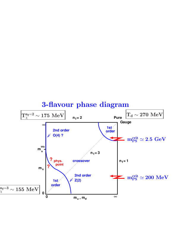
Figure 2: The QCD phase diagram of 3-flavor QCD with degenerate (u,d)-quark masses and a strange quark mass $m_{s}$.

The dependence of the QCD phase transition on the number of flavors and the values of the quark masses has been analyzed in quite some detail for vanishing values of the chemical potential. The current understanding of this phase diagram is summarized in Fig. 2. Its basic features have been established in numerical calculations and are in agreement with the general considerations based on universality and the symmetries of the QCD Lagrangian. Nonetheless, the numerical values for critical temperatures and critical masses given in this figure should just be taken as indicative; not all of them have been determined with sufficient accuracy. It is, however, obvious that there is a broad range of quark mass values or equivalently pseudo-scalar meson masses, where the transition to the high temperature regime is not a phase transition but a continuous crossover. The regions of first order transitions at large and small quark masses are separated from this crossover regime through lines of second order transitions which belong to the universality class of the 3d Ising model [15]. The chiral critical line in the small quark mass region has been analyzed in quite some detail [15, 16, 17]. In the case of three degenerate quark masses (3-flavor QCD) it has been verified that the critical point belongs to the Ising universality class [15]. The critical quark mass $m^{crit}$ at this point, however, is not a universal quantity and is not yet known to a satisfying precision: it corresponds to a pseudo-scalar mass varying between about 290 MeV in a standard discretization and about 200 MeV in an improved one. This result can be extended to the case of non-degenerate quark masses, i.e. $m_{s}\neq m_{l}$ where $m_{l}\equiv m_{u}=m_{d}$ denotes the value of the two light quark masses, which are taken to be degenerate. The slope of the chiral critical line in the vicinity of the three flavor point can be obtained from a Taylor expansion,

$$m^{crit}_{s}=m^{crit}+2\;(m^{crit}-m_{l})\quad.$$ (13)

This relation has been verified explicitly in a numerical calculation and is consistent with all existing studies of the chiral transition line [15, 16, 17]. A collection of results taken from Ref. [18] is shown in Fig. 3.

Figure 3: The chiral critical line in the light and strange quark mass plane. All the results shown have been obtained with a standard staggered fermion discretization [18].

If we assume that the linear extrapolation of the chiral critical line, Eq. 13, holds down to light quark mass values, which correspond to the physical pion mass, we estimate that the ratio of strange to light quark masses at this point is $(m^{crit}_{s}/m^{phys}_{l})_{\mu=0}\simeq 5-10$, depending on the action chosen. This clearly is too small to put the physical QCD point, which corresponds to $m_{s}/m_{u}\simeq 20$ into the first order regime of the phase diagram. At vanishing chemical potential the QCD transition thus most likely is a continuous crossover.

The phase diagram shown in Fig. 2 for vanishing quark chemical potential ($\mu$) can be extended to non-zero values of $\mu$. The chiral critical line discussed above then is part of a critical surface, $m^{crit}(\mu)$. For small values of the chemical potential it can be analyzed using a Taylor expansion of the fermion determinant in terms of $(\mu/T)$. A preliminary analysis performed for three flavor QCD [18] yields,

$$\biggl{(}{m^{crit}\over T}\biggr{)}_{\mu}=\biggl{(}{m^{crit}\over T}\biggr{)}_{0}+0.21(6)\;\biggl{(}{\mu\over T}\biggr{)}^{2}+{\cal O}((\mu/T)^{4})\quad,\quad n_{f}=3~{}.$$ (14)

The positive slope obtained for $m^{crit}(\mu)$ suggests that at the physical value of the strange quark mass a first order transition can occur for values of the chemical potential larger than a critical value determined from $m^{crit}(\mu)=m_{s}$ (see Fig. 4).

Figure 4: 3d sketch of the QCD phase diagram [18]: Shown is the critical surface of second order phase transition which separates the regime of first order phase transitions at large values of the chemical potential and/or small values of the light ($m_{u,d}$) and strange ($m_{s}$) quark masses from the regime of continuous, non-singular transitions (crossover) to the QCD plasma phase.

A first direct determination of the chiral critical point in QCD has been performed by Fodor and Katz [19]. As in the case of a Taylor expansion of the QCD partition functions in terms of the chemical potential, which we have discussed so far, they have also performed numerical calculations at $\mu=0$. However, they then evaluate the exact ratios of fermion determinants calculated at $\mu=0$ and $\mu>0$ and use these in the statistical reweighting of gauge field configurations to extend the calculation to $\mu\neq 0$. They find for the chiral critical point [20] $(\mu/T)_{crit}\simeq 1.4,~{}\mu^{crit}_{B}=3\mu^{crit}=(725\pm 35)$ MeV. Although this result still has to be established more firmly through calculations with lighter up and down quark masses on larger lattices and with improved actions, it also suggests that the dependence of the transition temperature on $\mu$ is rather weak.

An alternative approach to numerical calculations at non-zero values of the baryon number density ($\mu>0$) is based on numerical calculations with imaginary chemical potentials [22, 23, 24] ($\mu_{I}$). This allows straightforward numerical calculations for $\mu_{I}>0$. The results obtained in this way then have to be analytically continued to real values. For small values of the chemical potential which have been analyzed so far they turn out to be consistent with the results obtained with reweighting techniques.

Finally we want to note that the discussion of the dependence of the QCD phase diagram on the baryon chemical potential in general is a multi-parameter problem. As pointed out in Eq. 1 one generally has to deal with independent chemical potentials $\mu_{f}$ for each of the different quark flavors, which control the corresponding quark number densities,

$$d_{f}={1\over V}\;z_{f}\;{\partial\over\partial z_{f}}\ln Z(V,T,\mu_{f})\quad,\quad z_{f}={\rm e}^{\mu_{f}/T}\quad.$$ (15)

The chemical potentials thus are constrained by boundary conditions which are enforced on the quark number densities by a given physical system. In the case of dense matter created in a heavy ion collision this is $\mu_{s}=0$ due to the requirement that the overall strangeness content of the system vanishes. In a dense star, on the other hand, weak decays will lead to an equilibration of strangeness and it is the charge neutrality of a star which controls the relative magnitude of strange and light quark chemical potentials [25].

So far we have discussed a particular corner of the QCD phase diagram, i.e. the regime of small values of the chemical potential. In fact, the numerical techniques used today to simulate QCD with non-vanishing chemical potential seem to be reliable for $\mu/T\raise 1.29167pt\hbox{$<$\kern-7.5pt\raise-4.73611pt\hbox{$\sim$}}1$ and high temperature. Fortunately this is the regime, which also seems to be accessible experimentally. On the other hand there is the entire regime of low temperature and high density which is of great importance in the astrophysical context. In this regime it is expected that interesting new phases of dense matter exist. At low temperature and asymptotically large baryon number densities asymptotic freedom insures that the force between quarks will be dominated by one-gluon exchange. As this leads to an attractive force among quarks, it seems unavoidable that the naive perturbative ground state is unstable at large baryon number density and that the formation of a quark-quark condensate leads to a new color-superconducting phase of cold dense matter. As this part of the phase diagram is not in the focus of our following discussion we refer the interested reader to the many excellent reviews which appeared in recent years [26]. In Fig. 5 we just show a sketch of the phase diagram of QCD for a realistic quark mass spectrum. The transition to the plasma phase is expected to be a continuous crossover (dashed line) for small values of the quark chemical potential and turns into a first order transition only beyond a critical value for the chemical potential or baryon number density. The details of this phase diagram in particular in the low temperature regime are, however, largely unexplored in lattice calculations.

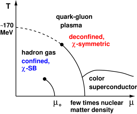
Figure 5: The QCD phase diagram in the $T-\mu$ as it might look like in the case of non-zero but light up and down quarks and a heavier strange quark.

3 The transition temperature

Although a detailed analysis of the QCD phase diagram clearly is of importance on its own, it is the thermodynamics in the region of small or vanishing chemical potential which is of most importance for a discussion of thermodynamic conditions created in heavy ion collisions at RHIC or LHC. Current estimates of baryon number densities obtained at central rapidities in heavy ion collisions at RHIC [27] suggest that the baryon chemical potential is below 50 MeV, corresponding to a quark chemical potential of about 15 MeV. We will see in the following that at these small values of $\mu$ the critical temperature is expected to change by less than a percent from that at $\mu=0$. For this reason, and of course also because much more quantitative results are known in this case, we will in the following focus our discussion on the thermodynamics at $\mu=0$.

As discussed in the previous section the transition to the high temperature phase is continuous and non-singular for a large range of quark masses. Nonetheless, for all quark masses the transition proceeds rather rapidly in a small temperature interval. A definite transition point thus can be identified, for instance through the location of maxima of the susceptibilities of the chiral condensate, $\chi_{m}$ (Eq. 7), or the Polyakov loop, $\chi_{L}$ (Eq. 10). While the maximum of $\chi_{m}$ determines the point of maximal slope in the chiral condensate, $\chi_{L}$ characterizes the change in the long distance behavior of the heavy quark free energy (see section 5).

On a lattice with temporal extent $N_{\tau}$ and for a given value of the quark mass the susceptibilities define pseudo-critical couplings $\beta_{pc}(m_{q},N_{\tau})$ which are found to coincide within statistical errors. In order to determine the transition temperature $T_{c}=1/N_{\tau}a(\beta_{pc})$ one has to fix the lattice spacing through the calculation of an experimentally or phenomenologically known observable. For instance, this can be achieved through the calculation of a hadron mass, $m_{H}a$, or the string tension, $\sigma a^{2}$, at zero temperature and the same value of the lattice cut-off, i.e. at $\beta_{pc}$. This yields $T_{c}/\sqrt{\sigma}=1/N_{\tau}\sqrt{\sigma a^{2}}$ and similarly for a hadron mass. In the pure gauge theory the transition temperature has been analyzed in great detail and the influence of cut-off effects has been examined through calculations on different size lattices and with different actions. From this one finds for the critical temperature of the first order phase transition

$$\underline{\rm SU(3)~{}gauge~{}theory:} T_{c}/\sqrt{\sigma}=0.632\pm 0.002$$ (16)

$$T_{c}=(269\pm 1)\;{\rm MeV}$$

Already the early calculations for the transition temperature in QCD with dynamical quark degrees of freedom [31, 32] indicated that the inclusion of light quarks leads to a significant decrease of the transition temperature. A compilation of newer results [32, 33, 34, 35, 36] which have been obtained using improved lattice regularizations for staggered as well as Wilson fermions is presented in Fig. 6. The figure only shows results for 2-flavor QCD obtained from calculations with several bare quark mass values. In order to compare calculations performed with different actions the results are presented in terms of a physical observable, the ratio of pseudo-scalar (pion) and vector (rho) meson masses, $m_{PS}/m_{V}$.

Figure 6: Transition temperature in 2-flavor QCD in units of $m_{V}$ calculated on lattices with temporal extent $N_{\tau}=4$ with different fermion actions. The large dot drawn for $m_{PS}/m_{V}=0$ indicates the result of chiral extrapolations based on calculations with improved Wilson [33] as well as improved staggered [35] fermions. The vertical line shows the location of the physical limit, $m_{PS}\equiv m_{\pi}=140~{}{\rm MeV}$.

From Fig. 6 it is evident that $T_{c}/m_{V}$ drops with increasing ratio $m_{PS}/m_{V}$, i.e. with increasing quark mass. This is not surprising as $m_{V}$, of course, does not take on the physical $\rho$-meson mass value as long as the quark masses used in the calculations are larger than than those realized in nature and the ratio $m_{PS}/m_{V}$ thus does not attain its physical value (vertical line in Fig. 6). In fact, for large quark masses $m_{V}$ will continue to increase with $m_{q}$ while $T_{c}$ will remain finite and eventually approach the value calculated in the pure $SU(3)$ gauge theory. The ratio $T_{c}/m_{V}$ has to approach zero for $m_{PS}/m_{V}=1$. Fig. 6 alone thus does not allow us to quantify the quark mass dependence of $T_{c}$.

A simple percolation picture for the QCD transition would suggest that $T_{c}(m_{q})$ or better $T_{c}(m_{PS})$ will increase with increasing $m_{q}$; with increasing $m_{q}$ all hadrons will become heavier and it will become more and more difficult to excite these heavy hadronic states. It thus becomes more difficult to create a sufficiently high particle/energy density in the hadronic phase that can trigger a phase (percolation) transition. Such a picture also follows from chiral model calculations [37, 38]. In order to check to what extent this physically well motivated picture finds support in the actual numerical results obtained in lattice calculations of the quark mass dependence of the transition temperature we should express $T_{c}$ in units of an observable, which itself is not (or only weakly) dependent on $m_{q}$; the string tension (or also a hadron mass in the valence quark chiral limit) seems to be suitable for this purpose. In fact, this is what we have tacitly assumed when converting the critical temperature of the SU(3) gauge theory, $T_{c}/\sqrt{\sigma}\simeq 0.63$, into physical units as it has been done in Eq. 16. This assumption is supported by the observation that already in the heavy quark mass limit the string tension calculated in units of quenched hadron masses, e.g. $m_{\rho}/\sqrt{\sigma}=1.81~{}(4)$ [39], is in good agreement with values required in QCD phenomenology, $\sqrt{\sigma}\simeq 425~{}{\rm MeV}$.

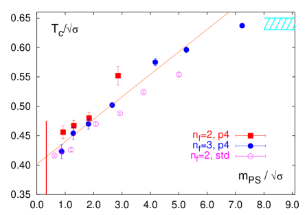
Figure 7: The transition temperature in 2 (filled squares) and 3 (circles) flavor QCD versus $m_{PS}/\sqrt{\sigma}$ using an improved staggered fermion action (p4-action). Also shown are results for 2-flavor QCD obtained with the standard staggered fermion action (open squares). The dashed band indicates the uncertainty on $T_{c}/\sqrt{\sigma}$ in the quenched limit. The straight line is the fit given in Eq. 18.

To quantify the quark mass dependence of the transition temperature one may express $T_{c}$ in units of $\sqrt{\sigma}$. This ratio is shown in Fig. 7 as a function of $m_{PS}/\sqrt{\sigma}$. As can be seen the transition temperature starts deviating from the quenched value for $m_{PS}\;\raise 1.29167pt\hbox{$<$\kern-7.5pt\raise-4.73611pt\hbox{$\sim$}}\;(6-7)\sqrt{\sigma}\simeq 2.5~{}{\rm GeV}$. We also note that the dependence of $T_{c}$ on $m_{PS}/\sqrt{\sigma}$ is almost linear in the entire mass interval. Such a behavior might, in fact, be expected for light quarks in the vicinity of a $2^{nd}$ order chiral transition where the dependence of the pseudo-critical temperature on the mass of the Goldstone-particle follows from the scaling relation

$$T_{c}(m_{\pi})-T_{c}(0)\sim m_{\pi}^{2/\beta\delta}~{}.$$ (17)

For 2-flavor QCD the critical indices $\beta$ and $\delta$ are expected to belong to the universality class of 3-d, $O(4)$ symmetric spin models and one thus indeed would expect to find $2/\beta\delta\simeq 1.1$. However, this clearly cannot be the origin for the quasi linear behavior which is observed already for rather large hadron masses and, moreover, seems to be independent of $n_{f}$. In fact, unlike in chiral models [37, 38] the dependence of $T_{c}$ on $m_{PS}$ turns out to be rather weak. The line shown in Fig. 7 is a fit to the 3-flavor data,

$$\biggl{(}{T_{c}\over\sqrt{\sigma}}\biggr{)}_{m_{PS}/\sqrt{\sigma}}=\biggl{(}{T_{c}\over\sqrt{\sigma}}\biggr{)}_{0}+0.04(1)\;\biggl{(}{m_{PS}\over\sqrt{\sigma}}\biggr{)}\quad.$$ (18)

It seems that the transition temperature does not react strongly to changes of the lightest hadron masses. This favors the interpretation that the contributions of heavy resonance masses are equally important for the occurrence of the transition. In fact, this also can explain why the transition still sets in at quite low temperatures even though all hadron masses, including the pseudo-scalars, attain masses of the order of 1 GeV or more. Such an interpretation also is consistent with the weak quark mass dependence of the critical energy density which one finds from the analysis of the QCD equation of state as we will discuss in the next section.

In Fig. 7 we have included results from calculations with 2 and 3 degenerate quark flavors. So far such calculations have mainly been performed with staggered fermions. In this case also a simulation with non-degenerate quarks (a pair of light u,d quarks and a heavier strange quark) has been performed. Unfortunately, the light quarks in this calculation are still too heavy to represent the physical ratio of light u,d quark masses and a heavier strange quark mass. Nonetheless, the results obtained so far suggest that the transition temperature in (2+1)-flavor QCD is close to that of 2-flavor QCD. The 3-flavor theory, on the other hand, leads to consistently smaller values of the critical temperature, $T_{c}(n_{f}=2)-T_{c}(n_{f}=3)\simeq 20$ MeV. Extrapolations of the transition temperatures to the chiral limit gave

$$\underline{\rm 2-flavor~{}QCD:} T_{c}=\cases{(171\pm 4)\;{\rm MeV},&clover-improved Wilson\cr~{}&fermions \cite[cite]{[\@@bibref{}{Ali01}{}{}]}\cr(173\pm 8)\;{\rm MeV},&improved staggered\cr~{}&fermions \cite[cite]{[\@@bibref{}{Kar01}{}{}]}\cr}$$

$$\underline{\rm 3-flavor~{}QCD:} T_{c}=\;\;\;\;(154\pm 8)\;{\rm MeV},\;\;\hskip 2.84544pt\mbox{improved staggered}$$

fermions [35]

Here $m_{\rho}$ has been used to set the scale for $T_{c}$. Although the agreement between results obtained with Wilson and staggered fermions is striking, one should bear in mind that all these results have been obtained on lattices with temporal extent $N_{\tau}=4$, i.e. at rather large lattice spacing, $a\simeq 0.3$ fm. Moreover, there are uncertainties involved in the ansatz used to extrapolate to the chiral limit. We thus estimate that the systematic error on the value of $T_{c}/m_{\rho}$ still is of similar magnitude as the purely statistical error quoted above.

As mentioned already in the previous section, first studies of the dependence of the transition temperature on the chemical potential have been performed recently using either a statistical reweighting technique [19, 20, 40] to extrapolate from numerical simulations performed at $\mu=0$ to $\mu>0$ or performing simulations with an imaginary chemical potential [23, 24] $\mu_{I}$ the results of which are then analytically continued to real $\mu$. To leading order in $\mu^{2}$ one finds

$${T_{c}(\mu)\over T_{c}(0)}=\cases{1-0.0056(4)(\mu_{B}/T)^{2}&Ref.~{}\cite[cite]{[\@@bibref{}{deForcrand}{}{}]} (imaginary $\mu$)\cr 1-0.0078(38)(\mu_{B}/T)^{2}&Ref.~{}\cite[cite]{[\@@bibref{}{Ejiri}{}{}]} (${\cal O}(\mu^{2}$) reweighting)}\quad.$$ (19)

These results are consistent with the (2+1)-flavor calculation performed with an exact reweighting algorithm [19, 20]. The result obtained for $T_{c}(\mu)$ in this latter approach is shown in Fig. 8. The dependence of $T_{c}$ on the chemical potential is rather weak. We stress, however, that these calculations have not yet been performed with sufficiently light up and down quark masses and a detailed analysis of the quark mass dependence has not yet been performed. The $\mu$-dependence of $T_{c}(\mu)/T_{c}(0)$ is expected to become stronger with decreasing quark masses (and, of course, vanishes in the limit of infinite quark masses).

Figure 8: The $\mu$-dependence of the transition temperature for (2+1)-flavor QCD [20].

4 The equation of state

One of the central goals in studies of the thermodynamics of QCD is, of course, the calculation of basic thermodynamic quantities and their temperature dependence. In particular, one wants to know the pressure and energy density which are of fundamental importance when discussing experimental studies of dense matter. Besides, they allow a detailed comparison of different computational schemes, e.g. numerical lattice calculations and analytic approaches in the continuum.

At high temperature one generally expects that due to asymptotic freedom these observables show ideal gas behavior and thus are directly proportional to the basic degrees of freedom contributing to thermal properties of the plasma, e.g. the asymptotic behavior of the pressure will be given by the Stefan-Boltzmann law

$$\lim_{T\rightarrow\infty}{p\over T^{4}}=(16+10.5n_{f}){\pi^{2}\over 90}\quad.$$ (20)

Perturbative calculations [41] of corrections to this asymptotic behavior are, however, badly convergent and suggest that a purely perturbative treatment of bulk thermodynamics is trustworthy only at extremely high temperatures, i.e. several orders of magnitude larger than the transition temperature to the plasma phase. In analytic approaches one thus has to go beyond perturbation theory which currently is being attempted by either using hard thermal loop resummation techniques in combination with a variational ansatz [42, 43] or perturbative dimensional reduction combined with numerical simulations of the resulting effective 3-dimensional theory [44, 45].

The lattice calculation of pressure and energy density is based on the standard thermodynamic relations given in Eq. 6. For vanishing chemical potential the free energy density is directly given by the pressure, $f=-p$. As the partition function itself is not directly accessible in a Monte Carlo calculation one first takes a suitable derivative of the partition function, which yields a calculable expectation value, e.g. the gauge action. After renormalizing this observable by subtracting the zero temperature contribution it can be integrated again to obtain the difference of free energy densities at two temperatures,

$$\frac{p}{T^{4}}{\biggl{|}}_{T_{o}}^{T}\;=\;{1\over V}\int_{T_{o}}^{T}{\rm d}t\;{\partial t^{-3}\ln Z(t,V)\over\partial t}\quad.$$ (21)

The lower integration limit $T_{o}$ is chosen at low temperatures so that $p/T_{o}^{4}$ is small and may be ignored. This easily can be achieved in an $SU(3)$ gauge theory where the only relevant degrees of freedom at low temperature are glueballs. Even the lightest ones calculated on the lattice have large masses, $m_{G}\simeq 1.5$ GeV. The free energy density thus is exponentially suppressed up to temperatures close to $T_{c}$. In QCD with light quarks, however, the dominant contribution to the free energy density comes from pions. In the small quark mass limit also $T_{o}$ has to be shifted to rather small temperatures. At present, however, numerical calculations are performed with rather heavy quarks and also the pion contribution thus is strongly suppressed below $T_{c}$.

In Fig. 9 we show results for the pressure obtained in calculations with different numbers of flavors [46]. At high temperature the magnitude of $p/T^{4}$ clearly reflects the change in the number of light degrees of freedom present in the ideal gas limit. When we rescale the pressure by the corresponding ideal gas values it becomes, however, apparent that the overall pattern of the temperature dependence of $p/T^{4}$ is quite similar in all cases. The figure also shows that the transition region shifts to smaller temperatures as the number of degrees of freedom is increased. As pointed out in the previous section such a conclusion, of course, requires the determination of a temperature scale that is common to all QCD-like theories which have a particle content different from that realized in nature. We have determined this temperature scale by assuming that the string tension is flavor and quark mass independent.

Figure 9: The pressure in QCD with two and three degenerate quark flavors as well as two light and a heavier (strange) quark [46]. For $n_{f}\neq 0$ calculations have been performed on an $N_{\tau}=4$ lattice using improved gauge and staggered fermion actions with a quark mass $m/T=0.4$. Cut-off effects in these calculations are expected to be of the order of 20% and the pressure is expected to become correspondingly larger once a proper extrapolation to the continuum limit can be performed on larger lattices. At high temperature the influence of a non-zero quark mass is expected to be small. In the case of the SU(3) pure gauge theory the continuum extrapolated result is shown.

Other thermodynamic observables can be obtained from the pressure using suitable derivatives. In particular one finds for the energy density,

$${\epsilon-3p\over T^{4}}=T{{\rm d}\over{\rm d}T}\left(\frac{p}{T^{4}}\right)\quad.$$ (22)

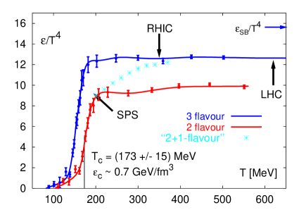
Figure 10: The energy density in QCD with 2 and 3 degenerate quark flavors. Also shown is a sketch of the expected form of the energy density for QCD with a fixed strange quark mass $m_{s}\sim T_{c}$ (see also remarks on cut-off effects in the caption of Fig. 9). The arrows indicating the energy densities reached in the initial stage of heavy ion collisions at the SPS, RHIC and in the future also at the LHC are based on the Bjorken formula [48].

In Fig. 10 we show results for the energy density obtained from calculations with staggered fermions and different number of flavors. Unlike the pressure the energy density rises rapidly at the transition temperature. Although the results shown in this figure correspond to quark mass values in the crossover region of the QCD phase diagram the transition clearly proceeds rather rapidly. This has, for instance, also consequences for the velocity of sound, $v_{s}^{2}=dp/d\epsilon$, which becomes rather small close to $T_{c}$. The velocity of sound is shown in Fig. 11. The comparison of results obtained from calculations in the $SU(3)$ gauge theory [28] and results obtained in simulations of 2-flavor QCD using Wilson fermions [47] with different values of the quark mass shows that the temperature dependence of $v_{s}$ is almost independent of the value of the quark mass.

Figure 11: The velocity of sound in the SU(3) gauge theory [28] and in 2-flavor QCD [47]. In the latter case we show results from calculations with Wilson fermions performed at different values of the quark mass.

Also shown in Fig. 10 is an estimate of the critical energy density at which the transition to the plasma phase sets in. In units of $T_{c}^{4}$ the transition takes place at $\epsilon/T_{c}^{4}\simeq 6\pm 2$ which should be compared with the corresponding value in the $SU(3)$ gauge theory [28], $\epsilon/T_{c}^{4}\simeq 0.5$. Although these numbers differ by an order of magnitude it is rather remarkable that the transition densities expressed in physical units are quite similar in both cases; when moving from large to small quark masses the increase in $\epsilon/T_{c}^{4}$ is compensated by the decrease in $T_{c}$. This result thus suggests that the transition to the QGP is controlled by the energy density, i.e. the transition seems to occur when the thermal system reaches a certain “critical” energy density. In fact, this assumption has been used in the past to construct the phase boundary of the QCD phase transition in the $T-\mu$ plane.

Also at non-vanishing baryon number density, the pressure as well as the energy density can be calculated along the same line outlined above by using the basic thermodynamic relation given in Eq. 6. Although the statistical errors are still large, a first calculation of the $\mu$-dependence of the transition line indeed suggests that $\epsilon(T_{c}(\mu),\mu)$ varies only little with increasing $\mu$, $\epsilon(T_{c}(\mu),\mu)-\epsilon(T_{c}(0),0)=(1.0\pm 2.2)\mu_{q}^{2}T_{c}^{2}(0)$ [40]. First calculations of the $\mu$-dependence of the pressure in a wider temperature range have recently been performed using the reweighting approach for the standard staggered fermion formulation [49] as well as the Taylor expansion for an improved staggered fermion action up to O($(\mu/T)^{4}$) [50]. This shows that the behavior of bulk thermodynamic observables follow a similar pattern as in the case of vanishing chemical potential. For instance, the additional contribution to the pressure, $\Delta p/T^{4}\equiv(p/T^{4})_{\mu/T}-(p/T^{4})_{\mu=0}$ rapidly rises at $T_{c}$ and shows only little temperature variation for $T/T_{c}\raise 1.29167pt\hbox{$>$\kern-7.5pt\raise-4.73611pt\hbox{$\sim$}}1.5$. In this temperature regime the dominant contribution to the pressure arises from the contribution proportional to $(\mu/T)^{2}$ which also is the dominant contribution in the ideal gas limit as long as $\mu/T\raise 1.29167pt\hbox{$<$\kern-7.5pt\raise-4.73611pt\hbox{$\sim$}}1$,

$$\biggl{(}{p\over T^{4}}\biggr{)}_{\mu/T}-\biggl{(}{p\over T^{4}}\biggr{)}_{\mu=0}={n_{f}\over 2}\biggl{(}{\mu\over T}\biggr{)}^{2}+{n_{f}\over 4\pi^{2}}\biggl{(}{\mu\over T}\biggr{)}^{4}\quad.$$ (23)

Here $(p/T^{4})_{\mu=0}$ is given by Eq. 20. It also turns out that at non-zero values of the chemical potential the cut-off effects in bulk thermodynamic observables are of the same size as at $\mu=0$. Further detailed studies of the behavior of the pressure and the energy density thus will require a careful extrapolation to the continuum limit and/or the use of improved gauge and fermion actions.

5 Heavy quark free energies

Heavy quark free energies play a central role in our understanding of the QCD phase transition, the properties of the plasma phase and the temperature dependence of the heavy quark potential. The heavy quark free energies [1] are defined as the QCD partition functions of thermal systems containing $n~{}(\bar{n})$ static quark (anti-quark) sources located at positions ${\bf x}=\{\vec{x}_{i}\}_{i=1}^{n}$ and $\bar{{\bf x}}=\{\bar{\vec{x}_{i}}\}_{i=1}^{\bar{n}}$,

$$Z^{(n,\bar{n})}(V,T,{\bf x},\bar{\bf x}) \equiv \exp(-F^{(n,\bar{n})}(V,T,{\bf x},\bar{\bf x})/T)$$

$$= \int{\cal D}A_{\nu}{\cal D}\bar{\psi}{\cal D}\psi\;{\rm e}^{-S_{E}(V,T,\mu_{f})}\prod_{i=1}^{n}{\rm Tr}\;L(\vec{x}_{i})\prod_{i=1}^{\bar{n}}{\rm Tr}\;L^{\dagger}(\bar{\vec{x}}_{i})~{},$$

where the Polyakov Loop, $L(\vec{x})$, has been defined in Eq. 9. The expectation value of the product of Polyakov loops gives the difference in free energy due to the presence of static $q\bar{q}$-sources in a thermal heat bath of quarks and gluons,

$$\biggl{\langle}\prod_{i=1}^{n}{\rm Tr}\;L(\vec{x}_{i})\prod_{i=1}^{\bar{n}}{\rm Tr}\;L^{\dagger}(\bar{\vec{x}}_{i})\biggr{\rangle} = {Z^{(n,\bar{n})}(V,T,{\bf x},\bar{\bf x})\over Z(V,T)}$$

$$= \exp(-\Delta F^{(n,\bar{n})}(V,T,{\bf x},\bar{\bf x})/T)$$

$$\equiv \exp(-(F^{(n,\bar{n})}(V,T,{\bf x},\bar{\bf x})-F(V,T))/T)~{},$$

where $Z(V,T)$ is the QCD partition function defined in Eq. 1. In particular, one considers the two point correlation function ($n=\bar{n}=1$),

$$G_{L}(|\vec{x}-\vec{y}|,T)=\langle{\rm Tr}\;L(\vec{x})\;{\rm Tr}\;L^{\dagger}(\vec{y})\rangle\quad,$$ (26)

and the Polyakov loop expectation value, which can be defined through the large distance behavior of $G_{L}$,

$$\langle L\rangle=\lim_{r\rightarrow\infty}\sqrt{G_{L}(r,T)}\quad,\quad r=|\vec{x}-\vec{y}|\quad.$$ (27)

These observables elucidate the deconfining features of the transition to the high temperature phase of QCD.

5.1 Deconfinement order parameter

The Polyakov loop expectation value has been introduced in Section 1 as an order parameter for deconfinement in the heavy quark mass limit of QCD, i.e. the $SU(3)$ gauge theory. Like in statistical models, e.g. the Ising model, it is sensitive to the spontaneous breaking of a global symmetry of the theory under consideration. In the case of the $SU(3)$ gauge theory this is the global $Z(3)$ centre symmetry [51]. In the presence of light dynamical quarks this symmetry is explicitly broken and in a strict sense the Polyakov loop looses its property as an order parameter. Through its relation to the two point correlation function, Eq. 27, it however still is the free energy of a static quark placed in a thermal heat bath,

$$F_{q}(T)=-T\ln(\langle L\rangle)\quad.$$ (28)

In the low temperature, confined regime $\langle L\rangle$ is small and the free energy thus is large. It is infinite only for an $SU(3)$ gauge theory, i.e. for QCD in the limit $m_{q}\rightarrow\infty$. In the high temperature regime however, $\langle L\rangle$ becomes large and $F_{q}$ decreases rapidly when crossing the transition region.

The static quark sources introduced in the QCD partition function through the line integral defined in Eq. 9 also introduce additional ultraviolet divergences, which require a proper renormalization. For the lattice regularized Polyakov loop this can be achieved through a renormalization of the temporal gauge link variables $U_{0}(n_{0},\vec{n})$, i.e.

$$L_{\vec{n}}\equiv\prod_{i=1}^{N_{\tau}}Z_{L}(g^{2})U_{0}(i,\vec{n})\quad~{}.$$ (29)

The renormalization constant $Z_{L}(g^{2})$ can, for instance, be determined by normalizing the two point correlation functions such that the resulting free energy of a color singlet quark anti-quark pair at short distances coincides with the zero temperature heavy quark potential. This also insures that divergent self energy contributions to the Polyakov loop expectation value, defined by Eq. 27, get removed and that the heavy quark free energy can unambiguously be defined also in the continuum limit [52].

We stress that it is conceptually appealing to define the renormalization constant for the Polyakov loop in terms of color singlet free energies. Nonetheless, this can also be achieved through the gauge invariant two point correlation functions, $G_{L}(r,T)$, which define so called color averaged free energies. A $q\bar{q}$-pair placed in a thermal heat bath cannot maintain its relative color orientation. The entire thermal system ($q\bar{q}$-pair $+$ heat bath) will be colorless and the $q\bar{q}$-pair can change its orientation in color space when interacting with gluons of the thermal bath. The Polyakov loop correlation function thus has to be considered as a superposition of contributions arising from color singlet ($F_{1}$) and color octet ($F_{8}$) contributions to the free energy [1],

$$\mbox{\rm e}^{-F^{(1,1)}(r,T)/T}=\frac{1}{9}\;\mbox{\rm e}^{-F_{1}(r,T)/T}+\frac{8}{9}\;\mbox{\rm e}^{-F_{8}(r,T)/T}\quad.$$ (30)

At short distances the repulsive octet term is exponentially suppressed and the contribution from the attractive singlet channel will dominate the heavy quark free energy,

$${F^{(1,1)}(r,T)\over T} = {F_{1}(r,T)\over T}\;-\;\ln 9$$ (31)

$$= -{g^{2}\over 3\pi}{1\over rT}\;-\;\ln 9\quad\quad{\rm for}\quad\;rT<<1\quad,$$

where the last equality gives the perturbative result obtained from 1-gluon exchange at short distances. When normalizing the color singlet free energy at short distances such that it coincides with the zero temperature heavy quark potential $V_{\bar{q}q}(r)$ the corresponding color averaged free energy thus will differ by an additive constant,

$$\lim_{r\rightarrow 0}(F^{(1,1)}(r,T)-F_{1}(r,T))=T\ln 9\quad{\rm for~{}all}~{}T.$$ (32)

Using this normalization condition the renormalized Polyakov loop order parameter has been determined for the $SU(3)$ gauge theory. It is shown in Fig. 12.

Figure 12: Temperature dependence of the renormalized Polyakov loop expectation value in the pure $SU(3)$ gauge theory determined from the asymptotic behavior of color singlet free energies on lattices of size $32^{3}\times N_{\tau}$.

As the deconfinement phase transition is first order in the $SU(3)$ gauge theory the order parameter is discontinuous at $T_{c}$. From the discontinuity, $\langle L\rangle(T_{c,+})\simeq 0.4$, one finds for the change in free energy $F_{\infty}(T_{c,+})\simeq 0.9T_{c}\simeq 250$ MeV.

In QCD with light quarks the renormalization program outlined above has not yet been performed in such detail as practically all studies of the heavy quark free energy have been performed on rather coarse lattices with a small temporal extent, $N_{\tau}=4$. Nonetheless, normalizing the free energies obtained in such calculations at the shortest distance presently available ($rT=1/N_{\tau}=0.25$) to the zero temperature Cornell potential does seem to be a reasonable approximation [53] (see Fig. 13). Also in this case the free energy at $T_{c}$ takes on a similar value as in the pure gauge theory.

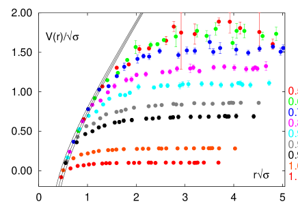
Figure 13: The color averaged heavy quark free energy ($V\equiv F^{(1,1)}$) at various temperatures in the low temperature phase of three flavor QCD (upper figure). The free energy has been normalized at the shortest distance available ($r=1/T$) to the zero temperature Cornell potential, $V(r)/\sqrt{\sigma}=-\alpha/r\sqrt{\sigma}+r\sqrt{\sigma}$ with $\alpha=0.25\pm 0.05$ (solid band). The lower figure shows the temperature dependence of the change in free energy when separating the quark anti-quark pair from a distance $r=0.5/\sqrt{\sigma}$ to infinity. To set the scale we use $\sqrt{\sigma}=425$ MeV.

5.2 Heavy quark potential

The change in free energy due to the presence of a static quark anti-quark pair is given by the two point correlation function defined in Eq. 26. In the zero temperature limit the free energies, $F^{(1,1)}(r,T)$, determined from $G_{L}(r,T)$ define the heavy quark potential. Also at non zero temperature the free energies exhibit properties expected from phenomenological discussions of thermal modifications of the heavy quark potential. In the pure gauge theory $m\rightarrow\infty$) the free energies diverge linearly at large distances in the low temperature, confinement phase. The coefficient of the linear term, the string tension at finite temperature, decreases with increasing temperature and vanishes above $T_{c}$. In the deconfined phase the free energies exhibit the behavior of a screened potential. At large distances they approach a constant value $F_{\infty}(T)$ at an exponential rate. This exponential approach defines a thermal screening mass. For finite quark masses the free energies show the expected string breaking behavior; at large distances they approach a finite value at all temperatures, i.e. also below $T_{c}$. This asymptotic value rapidly decreases with decreasing quark mass and increasing temperature [35] as can be seen in Fig. 13 where we show $F^{(1,1)}(r,T)$ in QCD with three light quark degrees of freedom [35]. In the lower part of Fig. 13 we show the change in free energy needed to separate a quark anti-quark pair from a distance typical for the radius of a $c\bar{c}$ bound state, i.e. $r=0.5/\sqrt{\sigma}\simeq 0.2$ fm, to infinity.

The change in free energy induced by a heavy quark anti-quark pair often is taken to be the heavy quark potential at finite temperature. Of course, this is not quite correct and care has to be taken when using the free energies in phenomenological discussions of thermal properties of heavy quark bound states. In this case we would like to know the energy needed to break up a color singlet state formed by a $\bar{q}q$-pair. As pointed out in the previous subsection, $F^{(1,1)}$ represents a color averaged free energy. It may be decomposed in terms of the corresponding singlet and octet contributions, which has indeed been done for $SU(2)$ and $SU(3)$ gauge theories [54, 55]. However, even then one has to bear in mind that the free energy is the difference between an energy and entropy contributions, $F=E-TS$. Of course, from a detailed knowledge of the temperature dependence of the free energy at fixed separation of the $\bar{q}q$-pair we can in principle determine the entropy and energy contributions separately,

$$S=-{\partial F(r,T)\over\partial T}\quad,\quad E=-T^{2}\;{\partial F(r,T)/T\over\partial T}\quad.$$ (33)

Such an analysis does, however, not yet exist.

6 Thermal modifications of hadron properties

6.1 QCD phase transition and the hadron spectrum

The non-perturbative structure of the QCD vacuum, in particular confinement and chiral symmetry breaking, determine many qualitative aspects of the hadron mass spectrum. Also the actual values of light and heavy quark bound state masses depend on the values of the chiral condensate and the string tension, respectively. As these quantities change with temperature and will change drastically close to the QCD transition temperature it also is expected that the properties of hadrons, e.g. their masses and widths, undergo drastic changes at finite temperature.

Investigations into the nature of hadronic excitations are interesting for various reasons in the different temperature regimes. Below $T_{c}$ temperature dependent modifications of hadron masses and widths may lead to observable consequences in heavy ion collision experiments e.g. a pre-deconfined dilepton enhancement due to broadening of the $\rho$-resonance or a shift of its mass [56]. At temperatures around the transition temperature the (approach to the) restoration of chiral symmetry should reflect itself in degeneracies of the hadron spectrum. First evidence for this has, indeed, been found early in lattice calculations of hadronic correlation functions [57]. In the plasma phase the very nature of hadronic excitations is a question of interest. Asymptotic freedom leads one to expect that the plasma consists of a gas of almost free quarks and gluons. The lattice results on the equation of state, however, have shown already that this is not yet the case for the interesting temperature region. While quasi-particle models and HTL resummed perturbation theory are able to reproduce the deviations from the ideal gas behaviour observed in the equation of state at temperatures a few times $T_{c}$ it remains to be seen whether they also account properly for hadronic excitations. This question arises in particular as the generally assumed separation of scales $1/T\ll 1/(gT)\ll 1/(g^{2}T)$ does not hold for temperatures quite a few times $T_{c}$.

In the previous section we have discussed modifications of the heavy quark free energy which indicate drastic changes of the heavy quark potential in the QCD plasma phase. As a consequence, depending on the quark mass, heavy quark bound states cannot form above certain “critical” temperatures [58]. Similarly it is expected that the QCD plasma cannot support the formation of light quark bound states. In the pseudo-scalar sector the disappearance of the light pions clearly is related to the vanishing of the chiral condensate at $T_{c}$. For $T>T_{c}$ the pions would be no longer (nearly massless) Goldstone bosons. In the plasma phase one thus may expect to find only massive quasi-particle excitations in the pseudo-scalar quantum number channel. However, also below $T_{c}$ it is expected that the gradual disappearance of the spontaneous breaking of chiral flavor symmetry as well as the gradual effective restoration of the axial $U_{A}(1)$ symmetry may lead to thermal modifications of hadron properties. While the breaking of the $SU_{L}(n_{f})\times SU_{R}(n_{f})$ flavor symmetry leads, for instance, to the splitting of scalar and pseudo-scalar particle masses, the $U_{A}(1)$ symmetry breaking is visible in the splitting of the pion and the $\eta^{\prime}$ meson.

More general, thermal modifications of the hadron spectrum should be discussed in terms of modifications of hadronic spectral functions which describe the thermal average over transition matrix elements between energy eigenstates ($E_{n}$) with fixed quantum numbers ($H$) [59],

$$\sigma_{H}(\omega,\vec{p},T)={1\over Z(T)}\sum_{n,m}e^{-E_{n}(\vec{p})/T}(1-e^{-\omega/T})\;\delta(\omega+E_{n}(\vec{p})-E_{m}(\vec{p}))\cdot$$

$${|\langle n|\hat{J}_{H}(0)|m\rangle|}^{2}\quad.$$ (34)

These spectral functions in turn determine the structure of Euclidean correlation functions, $G_{H}(\tau,\vec{x})$. Numerical studies of $G_{H}(\tau,\vec{x})$ at finite temperature thus will allow to learn about thermal modifications of the hadron spectrum, although in practice it is difficult to reconstruct the spectral functions themselves. Here recent progress has been reached through the application of the maximum entropy method (MEM). Before describing these developments and presenting recent lattice results we will start in the next subsection with a presentation of some basic field theoretic background on hadronic correlation functions and their spectral representation.

6.2 Spatial and temporal correlation functions, hadronic susceptibilities

6.2.1 Basic field theoretic background

Numerical calculations of hadronic correlation functions are carried out on Euclidean lattices i.e. one uses the imaginary time formalism. This holds also for zero temperature computations in which case the $T\rightarrow 0$ limit has to be taken. The formalism has been worked out in detail in textbooks [7, 59, 60], however, for readers’ convenience we have collected some formulae in the Appendix.

Hadronic correlation functions in coordinate space, $G_{H}(\tau,\vec{x})$, are defined as

$$G_{H}(\tau,\vec{x}) = \langle J_{H}(\tau,\vec{x})J_{H}^{\dagger}(0,\vec{0})\rangle$$ (35)

where the hadronic, e.g. mesonic, currents $J_{H}(\tau,\vec{x})=\bar{q}(\tau,\vec{x})\Gamma_{H}q(\tau,\vec{x})$ contain an appropriate combination of $\gamma$-matrices, $\Gamma_{H}$, which fixes the quantum numbers of a meson channel; i.e., $\Gamma_{H}=1$, $\gamma_{5}$, $\gamma_{\mu}$, $\gamma_{\mu}\gamma_{5}$ for scalar, pseudo-scalar, vector and pseudo-vector channels, respectively.

On the lattice, at zero temperature, one usually studies the temporal correlator at fixed momentum $\vec{p}$. Save possible subtractions, the correlator is related to the spectral function (see Appendix), $\sigma_{H}(p_{0},\vec{p})$, by means of

$$G^{T}_{H}(\tau,\vec{p})=\int_{0}^{+\infty}dp_{0}\,\sigma_{H}(p_{0},\vec{p})K(p_{0},\tau)\quad,$$ (36)

where the kernel

$$K(p_{0},\tau)=\frac{\cosh[p_{0}(\tau-1/2T)]}{\sinh(p_{0}/2T)}$$ (37)

describes the propagation of a single free boson of mass $M\equiv p_{0}$. At zero temperature, for large temporal separations the correlation function is dominated by the exponential decay due to the lightest contribution to the spectral function in a given channel.

At finite temperature, studies of the temporal correlator are hampered by the limited extent of the system in the time direction. Therefore most (lattice) analyses have been concentrating on the spatial correlation functions. These depend of course on the same (temperature dependent) spectral density but are different Fourier transforms of it. Projecting onto vanishing transverse momentum and vanishing Matsubara frequency one obtains

$$G^{S}_{H}(z)=\int_{-\infty}^{+\infty}\frac{dp_{z}}{2\pi}\,e^{ip_{z}z}\,\int_{-\infty}^{+\infty}dp_{0}\frac{\sigma_{H}(p_{0},\vec{0}_{\perp},p_{z})}{p_{0}}~{}~{}.$$ (38)

In addition it is quite common in lattice calculations to analyze hadronic susceptibilities which are given by the space-time integral over the Euclidean correlation functions,

$$\chi_{H} = \int_{0}^{1/T}d\tau\;G^{T}_{H}(\tau,\vec{0})\quad.$$ (39)

The susceptibilities have a particularly simple relation to the spectral function,

$$\chi_{H}=2\int_{0}^{\infty}dp_{0}\frac{\sigma_{H}(p_{0},\vec{0})}{p_{0}}~{}~{}.$$ (40)

Unfortunately, these susceptibilities are generally ultraviolet divergent and the above defined integrals should be cut-off at some short distance scale. Rather than doing this one can consider a closely related quantity, which provides a smooth, exponential cut-off for the ultraviolet part of the spectral function and is given by the thermal correlation function at $\tau T=1/2$,

$$G^{T}_{H}(1/2T,\vec{0})=\int_{0}^{\infty}dp_{0}\frac{\sigma_{H}(p_{0},\vec{0})}{\sinh(p_{0}/2T)}\quad.$$ (41)

In the case of a free stable boson of mass $M_{H}$ the spectral function is a pole

$$\sigma_{H}(p_{0},\vec{p})=\;|\langle 0|J_{H}|H(\vec{p})\rangle|^{2}\;\epsilon(p_{0})\delta(p_{0}^{2}-\vec{p}^{\,2}-M^{2}_{H})\quad.$$ (42)

Correspondingly, the imaginary time correlator, projected to vanishing momentum, decreases with the mass (modulo periodicity) as

$$G^{T}_{H}(\tau,\vec{0})\sim\frac{1}{2M_{H}}\frac{\cosh[M_{H}(\tau-1/2T)]}{\sinh(M_{H}/2T)}\quad.$$ (43)

Likewise, in this case the spatial correlator is also decaying with the mass

$$G^{S}_{H}(z)\sim\frac{1}{2M_{H}}\exp(-M_{H}z)\quad.$$ (44)

In this simple case the exponential fall-off of spatial and temporal correlation functions thus carry the same information on the particle mass. Interactions in a thermal medium, however, are likely to alter the dispersion relation to

$$\omega^{2}(\vec{p},T)=M^{2}_{H}+{\vec{p}}^{\,2}+\Pi(\vec{p},T)$$ (45)

with the temperature dependent vacuum polarization $\Pi(\vec{p},T)$. In the simplest case, one can perhaps assume [61] that the temperature effects can be absorbed into a temperature dependent mass $M_{H}(T)$ and a coefficient $A(T)$ which might also be temperature dependent and different from 1,

$$\omega^{2}(\vec{p},T)\simeq M^{2}_{H}(T)+A^{2}(T){\vec{p}}^{\,2}$$ (46)

In this case, at zero momentum the temporal correlator will decay with the so-called pole mass $M_{H}(T)$,

$$G^{T}_{H}(\tau,\vec{0})\sim\exp(-M_{H}(T)\tau)\quad,$$ (47)

whereas the spatial correlation function has an exponential fall-off,

$$G^{S}_{H}(z)\sim\exp(-M^{\rm sc}_{H}(T)z)\quad,$$ (48)

determined by the screening mass $M^{\rm sc}_{H}(T)=M_{H}(T)/A(T)$ which differs from the pole mass if $A(T)\neq 1$. In this simple case also the susceptibility defined in Eq. 39 as well as the central value of the temporal correlation function defined in Eq. 41 are closely related to the pole mass,

$$\chi_{H} \sim \frac{1}{M^{2}_{H}(T)}\quad,$$

$$G^{T}_{H}(\tau=1/2T,\vec{0}) \sim \frac{1}{M_{H}(T)\sinh(M_{H}(T)/2T)}\quad,$$ (49)

respectively.

The opposite limit to the case of a free stable boson is reached for two freely propagating quarks contributing to the spectral density. Here, to leading order perturbation theory the evaluation of the meson correlation function amounts to the evaluation of the self-energy diagram shown in Fig. 14a in which the internal quark lines represent bare quark propagators $S_{F}(i\omega_{n},\vec{p})$ [63].

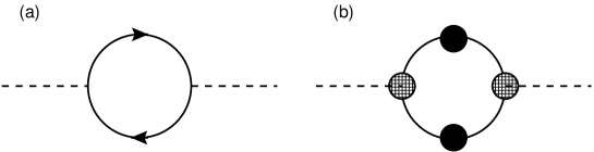
Figure 14: The self-energy diagrams for free quarks (a) and in the HTL approximation (b).

Table 1: Coefficients $a_{H}$ and $b_{H}$ for the free continuum as well as coefficients $a_{H}^{\rm lat}$ and $d_{H}^{\rm lat}$ for the free lattice correlation function, Eqs. 51,58, in the various channels. $d$ is given by $A/\sinh^{2}E$.

$H$	$a_{H}$	$b_{H}$	$a_{H}^{\rm lat}$	$d_{H}^{\rm lat}$
$PS$	1	0	1	0
$S$	-1	1	-d	d-1
$\sum_{i=1}^{3}V_{i}$			3-d	d
$V_{0}$			0	-1
$\sum_{\mu=0}^{3}V_{\mu}$	2	1	3-d	d-1
$\sum_{i=1}^{3}AV_{i}$			-2d	2d-3
$AV_{0}$			1-d	d
$\sum_{\mu=0}^{3}AV_{\mu}$	-2	3	1-3d	3(d-1)

For massless quarks the spectral density in the mesonic channel $H$ is then computed from Eq. LABEL:eq:freequarkprop_2 as,

$$\sigma_{H}(p_{0},\vec{p})=\frac{N_{c}}{8\pi^{2}}\,(p_{0}^{2}-\vec{p}^{\,2})\,a_{H}\,\left\{\Theta(p_{0}^{2}-\vec{p}^{\,2})\,\frac{2T}{p}\ln\frac{\cosh(\frac{p_{0}+p}{4T})}{\cosh(\frac{p_{0}-p}{4T})}\right.$$

$$+\left.\Theta(\vec{p}^{\,2}-p_{0}^{2})\left[\frac{2T}{p}\ln\frac{\cosh(\frac{p+p_{0}}{4T})}{\cosh(\frac{p-p_{0}}{4T})}-\frac{p_{0}}{p}\right]\right\}$$ (50)

where $p=\sqrt{\vec{p}^{\,2}}$ and $a_{H}$ depends on the channel analyzed (see Table 1 for some selected values). In the limit of vanishing momentum $\vec{p}$ the spectral density is also known [64] for quarks with non-vanishing masses $m$,

$$\sigma_{H}(p_{0},\vec{0})=\frac{N_{c}}{8\pi^{2}}\,p_{0}^{2}\,\Theta(p_{0}^{2}-4m^{2})\tanh\left(\frac{p_{0}}{4T}\right)\sqrt{1-\left(\frac{2m}{p_{0}}\right)^{2}}$$

$$\left[a_{H}+\left(\frac{2m}{p_{0}}\right)^{2}b_{H}\right]\quad.$$ (51)

The coefficients $b_{H}$ are also given in Table 1. For massless quarks closed analytic expressions can be given for both, the temporal as well as the spatial correlator, e.g. for the pion [63]

$$G^{T,\rm free}_{\pi}(\tau,\vec{0})/T^{3}=\pi N_{c}(1-2\tau T)\frac{1+\cos^{2}(2\pi T\tau)}{\sin^{3}(2\pi T\tau)}+2N_{c}\frac{\cos(2\pi T\tau)}{\sin^{2}(2\pi T\tau)}$$ (52)

$$G^{S,\rm free}_{\pi}(z) = \frac{N_{c}T}{4\pi z^{2}\sinh(2\pi Tz)}[1+2\pi Tz\,\coth(2\pi Tz)]$$ (53)

$$\sim e^{-M_{sc}^{free}z}\quad{\rm with}\quad M_{sc}^{free}=2\pi T\quad.$$

In this free field limit the susceptibility $\chi_{H}$, defined in Eq. 39, is divergent, while the temporal correlator at $\tau T=1/2$, of course, stays finite

$$G^{T,\rm free}_{H}(1/2,\vec{0})/T^{3}=a_{H}N_{c}/3\quad.$$ (54)

It, however, is neither related to the screening mass nor does this finite value have anything to do with the existence of a pole mass.

The above discussion can be extended to the leading order hard thermal loop (HTL) approximation [64] using dressed quark propagators and vertices for the calculation of the self-energy diagrams as indicated in Fig. 14b. The corresponding quark spectral functions are given in the Appendix.

In the interacting case it has been argued [65] from dimensionally reduced QCD that the simple relation between screening mass and lowest Matsubara frequency will be changed, to leading order, into

$$M_{\rm sc}(T)=2\pi T+\frac{C_{F}}{4\pi}g^{2}(T)T\left[2-\ln\frac{C_{F}g^{2}(T)}{4\pi^{2}}\right]\quad.$$ (55)

Further corrections are expected to arise from non-perturbative effects, e.g. from the fact that space-like Wilson loops obey an area law [66]. Correspondingly, the logarithmic potential used to arrive at the estimate given in Eq. 55 will turn into a linear rising one at large distances. The effect of this is expected to be marginal on the screening mass, however, will be large for so-called spatial wave functions.

6.2.2 Lattice results

As has been mentioned already in the previous section, the temporal separation of the operators is limited by the inverse temperature and the traditional approach of extracting a ground state mass from the long distance behavior of a Euclidean correlation function thus is not possible. Many lattice studies therefore have concentrated on the analysis of spatial correlation functions. As outlined in the previous section the exponential decrease in the spatial distance then defines a screening mass, which in certain limiting cases indeed may be related to the pole mass.

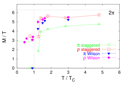
Figure 15: Screening masses in quenched QCD [69, 70] calculated with Wilson and staggered fermions. Below $T_{c}$ the masses are normalized to $T_{c}$, above to $T$.

Fig. 15 shows one representative set of lattice results on screening masses calculated in the quenched approximation and using the Wilson as well as the staggered discretization scheme for the fermion action. So far, below $T_{c}$ the screening masses themselves have not shown any significant temperature dependence. This holds for quenched staggered [67] and Wilson [61, 68, 69, 70] as well as for dynamical quarks [71, 72]. Thus, there also is no substantial difference between the screening and the zero temperature masses. This seems to be in accord with sum rule predictions [73] but in conflict with chiral perturbation theory [74]. It has been argued [75] that the masses should have the same temperature dependence as the chiral condensate. However, also the lattice results for this quantity when normalized to its zero temperature value do not exhibit marked deviations from unity up to temperatures close to $T_{c}$, see Fig. 16. Here it may be of particular importance to perform numerical calculations with lighter dynamical quark masses in order to get better control over the influence of light virtual quarks on the chiral condensate and the resonance decay of hadronic bound states.

Figure 16: The chiral condensate normalized to its zero temperature value for a variety of flavor numbers.

At temperatures (slightly) above $T_{c}$ the temporal and spatial correlation functions of chiral partners reflect the restoration of chiral $SU_{L}(n_{f})\times SU_{R}(n_{f})$ symmetry. In particular, the vector and axial vector channel become degenerate [57, 61, 68, 69, 70, 71, 72, 76, 77, 78, 79, 80, 81], independent of the discretization and of the number of dynamical flavors being simulated. The same degeneracy is observed within errors in the pseudo-scalar and isoscalar scalar ($\sigma/f_{0}$) channel although the latter, for technical reasons, is difficult to access on the lattice. Nevertheless, screening masses obtained from fits to correlation functions [82] and susceptibilities (at finite lattice spacing) [83, 84] lead to a consistent picture.

A more intricate question is the one concerning the degeneracy of the pseudo-scalar and scalar isovector ($\delta/a_{0}$) channel [85]. In three-flavor QCD this degeneracy follows already from the above mentioned chiral one. For two flavors in the chiral limit it detects the effective restoration of the anomalous $U_{A}(1)$. Although the $U_{A}(1)$ is explicitly broken by perturbative quantum effects it might become effectively restored non-perturbatively if topologically non-trivial zero-modes of the Dirac-matrix are absent. If this happens already at temperatures below or at $T_{c}$ the chiral transition for two flavors will even be first order [13]. Getting control over the zero-modes in lattice calculations is, however, complicated. They are particularly sensitive to discretization effects and the continuum as well as the chiral limit have to be controlled. The use of improved actions with better chiral properties at finite lattice spacing thus is important and the most convincing evidence so far has therefore been obtained in calculations with the domain wall fermion discretization [86] (see Fig. 17). This study suggests that the $U_{A}(1)$ symmetry is not yet restored effectively at the transition temperature, a conclusion which was cautiously drawn also from earlier attempts utilizing standard staggered actions [79, 82, 83, 84, 87].

Figure 17: The difference of the $\pi$ and $\delta$ susceptibility in two-flavor QCD as function of the quark mass in lattice units. The data [86] were obtained at two values of the coupling constant which correspond to temperatures slightly above $T_{c}$. The lines are fits of the form $c_{0}+c_{2}m_{f}^{2}$ which is the quark mass dependence expected in the continuum. A vanishing intercept in the chiral limit would support effective $U_{A}(1)$ restoration.

At high temperature, the screening masses are expected to approach the free quark propagation limit, Eq. 53. In fact, already at temperatures as low as about 1.5 $T_{c}$, the results for the vector channel are close to this value, $M_{sc}=2\pi T$. Nonetheless, Fig. 15 still indicates some 10 - 15 % deviations from free quark behavior which are of similar size than e.g. in the equation of state. As such, the degeneracy between pseudo-scalar and vector channels in the Wilson discretization [68, 69] is not seen for staggered quarks. However, these results were not yet attempted to be extrapolated to the continuum limit and it is thus interesting that a recent paper [81] reports that also in the latter discretization this degeneracy is reached in the continuum limit.

Apart from screening masses, also the temperature dependence of spatial wave functions has been investigated [69, 77]. Also in this quantity, significant differences to zero temperature results could not be detected for temperatures $T\raise 1.29167pt\hbox{$<$\kern-7.5pt\raise-4.73611pt\hbox{$\sim$}}T_{c}$. Above the critical temperature, the spatial wave functions become narrower with increasing temperature. Qualitatively, this observation is in accord [90] with a rising spatial string tension [28, 89]. However, a quantitative comparison is still lacking.

Attempts to extract masses, rather than screening masses, from fits to temporal correlation functions have used extended operators of various kinds possibly combined with anisotropic lattices [61, 68, 78]. Both methods are means to counteract the short extent in the temperature direction. In the first case one hopes for a ground state contribution (if any) dominating already at small temporal distances. In the second case the isolation of the lowest lying state may be helped by the increased number of data points stabilizing more sophisticated fit ansätze which include more than a ground state contribution. However, one still has to rely on fit ansätze and, if possible, use the quality of the fit to distinguish between the various models. Moreover, modelling the operators introduces biases. The results have thus turned out to depend somewhat on the method. In general, they are at least qualitatively in agreement with an important two-quark cut contribution. In addition, the behavior of wave functions was interpreted to indicate meta-stable bound states [68]. In any case, the existence of genuine, narrow bound-states above $T_{c}$ could be excluded.

Figure 18: Temporal (left) pseudo-scalar correlation functions at temperatures below and above $T_{c}$. Below $T_{c}$ the correlation function for one value of the quark mass is shown whereas above $T_{c}$ simulations have been performed in the chiral limit. The right hand figure shows the chiral extrapolation of the central value of the temporal pseudo-scalar correlator below $T_{c}$. The bars denote value and error of the critical hopping parameter obtained from the chiral extrapolation of pseudo-scalar screening masses.

6.3 Spectral functions from hadronic correlation functions

The discussion in the previous section shows that we have evidence from numerical calculations that the spectral properties of hadrons change with temperature. The drastic changes of hadronic correlation functions that occur when one crosses the transition temperature to the high temperature plasma phase are self-evident from the changes in the screening masses. The temperature dependence of correlation functions is particularly striking in the pseudo-scalar channel (see Fig. 18). Below $T_{c}$ the central value, $G_{PS}(\tau T=1/2,T)$, diverges in the chiral limit, which reflects that the pseudo-scalar remains massless (Eq. 49), and above $T_{c}$ it stays finite and comes close to the free field limit.

A much more subtle question is to quantify which thermal modifications of the spectral functions lead to the observed modification of the correlation functions. In order to decide on this we would like to have a more direct access to the spectral functions. It has been suggested recently [91] to apply the Maximum Entropy Method (MEM), a well known statistical tool for the analysis of noisy data [92], also to the analysis of hadronic correlation functions. At least in principle, i.e. given sufficiently accurate numerical data on large lattices, this approach allows to extract detailed information on hadronic spectral functions at zero as well as finite temperature.

A lattice calculation of a hadronic correlation function on a lattice with temporal extent $N_{\tau}$ provides a set of data, $\displaystyle{\{G_{H}(\tau_{i})_{j}\}^{j=1,N_{D}}_{i=1,N_{\tau}}}$, where $N_{D}$ denotes the number of measurements of a correlation function at a discrete set of Euclidean times $\tau_{i}T=i/N_{\tau},~{}i=1,..,N_{\tau}$. The statistical analysis of this data set based on MEM aims at a determination of the most likely spectral function which describes the data given any prior knowledge on the correlation function or the spectral function. This information is taken into account in the so-called default model. In the case of hadronic correlation functions one usually tries to provide in this way information on the perturbatively known short distance behavior of Euclidean correlation functions. The first studies of spectral functions based on the MEM approach [91] and in particular the analysis of simple toy models at zero [91, 94] and finite temperature [95] have, indeed, been encouraging. The MEM approach has since then been used and further tested in various studies of hadronic correlation functions at zero and finite temperature both for light and heavy quarks [94, 96, 97, 98, 99, 100, 101, 102]. We will discuss some of the results in the following. More details on the maximum entropy methods and its utilization for lattice QCD calculations are given in Ref. [93].

To illustrate the kind of thermal modifications of Euclidean correlation and spectral functions and the way this is analyzed using MEM let us briefly discuss some basic aspects of the correlation and spectral functions at zero and non-zero temperature. To be specific we consider the vector channel. The case of a freely propagating quark anti-quark pair is of relevance for the short distance part of the correlation functions as well as in the high (infinite) temperature limit. For massless quarks the corresponding spectral functions are given by Eq. 51,

$$\sigma_{V}(p_{0},\vec{0})=\cases{\frac{N_{c}}{4\pi^{2}}\,p_{0}^{2}&$T=0$\cr\frac{N_{c}}{4\pi^{2}}\,p_{0}^{2}\,\tanh\left(\frac{p_{0}}{4T}\right)&$T>0$}\quad.$$ (56)

The corresponding correlation functions are shown in the left hand part of Fig. 19. Note that the spectral functions for $T=0$ as well as $T>0$ are scale invariant, i.e. the rescaled spectral functions, $\sigma_{V}/T^{2}$, depend on the rescaled energies, $p_{0}/T$, only. As a consequence the rescaled correlation functions $G_{V}/T^{3}$ are also scale invariant and are functions of $\tau T$ only. As a first test for the MEM analysis we may provide a set of data corresponding to the $T>0$ correlation function shown in Fig. 19 (left) and use the $T=0$ spectral function as a default model. As can be seen in Fig. 19 (right) the MEM analysis indeed can reproduce the thermal modification of the spectral functions already with a rather small set of equally spaced data points [95] and, in turn, yields a perfect reconstruction of the correlation function.

Figure 19: Correlation functions for a free quark anti-quark pair (left) and the corresponding spectral functions (right). The boxes indicate 32 equally spaced points on the free correlation function for $T>0$. The curve through these points is obtained from the reconstructed spectral function. The upper curve in the left hand figure and the straight line in the right hand figure correspond to the input default model for the MEM analysis.

At zero temperature, the free spectral function (Fig. 19), only characterizes the short distance behavior of the correlation function or the large energy behavior of the spectral function, respectively. The most prominent modification, of course, results from the presence of the $\rho$-resonance and a more realistic spectral function is [104],

$$\sigma_{\rho_{i}}(p_{0},\vec{0}) = \frac{2p_{0}^{2}}{\pi}\biggl{[}F_{\rho}^{2}{\Gamma_{\rho}m_{\rho}\over(p_{0}^{2}-m_{\rho}^{2})^{2}+\Gamma_{\rho}^{2}m_{\rho}^{2}}$$ (57)

$$\hskip 14.22636pt+\frac{1}{8\pi}\biggl{(}1+\frac{\alpha_{s}}{\pi}\biggr{)}{1\over 1+{\rm exp}((\omega_{0}-p_{0})/\delta)}\biggr{]}\quad,$$

with $\Gamma_{\rho}=m_{\rho}^{3}/(48\pi F_{\rho}^{2})$ in the chiral ($m_{\pi}=0$) limit and $m_{\rho}=770$ MeV, $F_{\rho}=142$ MeV, $\omega_{0}=1.3$ GeV, $\delta=0.2$ GeV and $\alpha_{s}=0.3$. Due to the explicit appearance of hadronic scales this spectral function, of course, is no longer scale invariant in the sense introduced above. Assuming Eq. 57 to hold also at non-zero temperature thus will also lead to vector correlation functions which are no longer scale invariant. In Fig. 20 we show the scaled vector meson correlation functions, $G_{\rho}(\tau T)/T^{3}$, for temperatures $T=0.1,~{}0.2$ and 1 GeV. The temperature dependence of the correlation function is apparent. At the highest temperature $G_{\rho}(\tau T)/T^{3}$ almost coincides with the corresponding rescaled free, zero temperature, correlation function. This shows that at these high temperatures the structure of the correlation function is dominated by the high energy part of the continuum contribution; the contribution of the $\rho$-resonance is suppressed.

Figure 20: Vector meson correlation functions at temperatures below and above $T_{c}$ constructed from a phenomenological zero temperature vector meson spectral function.

The scaling violations visible in Fig. 20 are most prominent for $\tau T\simeq 0.5$, which reflects that the hadronic scales, which violate the scaling of the spectral functions with temperature, show up at low energies. This is quite distinct from finite-cut off effects on the lattice that result in a distortion of the high energy part of the spectral functions and consequently lead to a modification of correlation functions at short distances.

On finite lattices the temporal correlation functions built from free, massless quark propagators in the Wilson discretization [105] are given by a sum over the quark momenta $\vec{k}$, at zero spatial “meson” momentum

$$G_{H}^{\rm free,lat}(\tau,\vec{0})/T^{3}=N_{c}\left(\frac{N_{\tau}}{N_{\sigma}}\right)^{3}\sum_{\vec{k}}\frac{1}{(1+B)^{2}}\frac{1}{\cosh^{2}(EN_{\tau}/2)}~{}\cdot$$

$$\left\{a_{H}^{\rm lat}\cosh[2E(\tau-N_{\tau}/2)]+d_{H}^{\rm lat}\right\}\quad.$$ (58)

Here, $B$ is given by $B=2\sum_{i}\sin^{2}(k_{i}/2)$ and $E$ denotes the quark energy $E=2\ln\left\{\sqrt{\alpha/4}+\sqrt{1+\alpha/4}\right\}$ with $\alpha=(A+B^{2})/(1+B)$ where $A=\sum_{i}\sin^{2}k_{i}$. The coefficients $a_{H}^{\rm lat}$ and $d_{H}^{\rm lat}$ are collected in Table 1 for some channels $H$. Note that the coefficient $d_{H}^{\rm lat}$ approaches 1 in the continuum limit. Moreover, in the zero temperature limit, the $\tau$ independent piece of the correlation function $G_{H}^{\rm free,lat}(\tau,\vec{0})$ vanishes proportional to $T^{3}$. In Fig. 21 we show the free vector correlation functions and the corresponding spectral functions [103] on lattices with temporal extent $N_{\tau}=16$, 24 and 32. As can be seen the influence of finite cut-off effects is restricted to the short distance behavior of the correlation functions, which results from the strict momentum cut-off on a finite lattice. We also note the pronounced peak in the lattice spectral function, which results from the distortion of the lattice dispersion relation for free quarks at large momentum and, in particular, close to the corners of the first Brillouin zone. In the interacting case peaks at $ap_{0}\simeq 2$ thus have been attributed to the influence of the heavy Wilson doublers [94].

Figure 21: Free pseudo-scalar correlation functions (left) and spectral functions (right) calculated on lattices with temporal extent $N_{\tau}$ using the Wilson fermion formulation.

6.4 Spectral analysis of thermal correlation functions

In Section 6.3 we have discussed properties of the pseudo-scalar correlation functions below and above $T_{c}$ which clearly suggest that the spectral properties in this channel drastically change when going from the low temperature hadronic phase to the high temperature plasma phase. After this drastic change the rescaled pseudo-scalar correlation function above $T_{c}$, however, seems to be only weakly temperature dependent. This property is even more pronounced in the vector channel. In Fig. 22 we show the vector correlation function for a set of temperatures ranging from $0.4\;T_{c}$ up to $3\;T_{c}$ calculated on lattices of size up to $64^{3}\times 16$. As can be seen the rescaled correlation functions are within statistical errors temperature independent. In view of the discussion presented in the previous section this is indeed remarkable; the scaling of the correlation function is inconsistent with a temperature independent spectral function and, in fact, suggests that also the parameters determining the spectral function (or at least its dominant part) scale with temperature.

Figure 22: Vector meson correlation functions at various temperatures below and above $T_{c}$. For better visibility data points have slightly been shifted horizontally relative to the data set at $T=0.4T_{c}$.

As at high temperature the vector spectral function is dominated by the continuum contribution the most obvious expectation is that the parameters controlling the threshold in the continuum contribution, $\omega_{0}$ and $\delta$, increase with temperature.

The existence of a temperature dependent energy cut-off in the vector as well as the pseudo-scalar spectral functions above $T_{c}$ is also obtained in the MEM analysis of the corresponding correlation functions. This is shown in Fig. 23. In both cases the reconstructed spectral functions suggest that the contributions from the pion and rho states disappear above $T_{c}$. Instead, a broad peak becomes visible which shifts to larger energies with increasing temperature.

Figure 23: Pseudo-scalar (left) and vector (right) spectral functions obtained from quenched QCD calculations on lattices up to size $64^{3}\times 16$ using improved Wilson fermions.

6.5 Vector meson spectral function and thermal dilepton rates

The vector spectral function shown in Fig. 23 is directly related to the thermal cross section for the production of dilepton pairs at vanishing momentum,

$${{\rm d}W\over{\rm d}p_{0}{\rm d}^{3}p}|_{\vec{p}=0}={5\alpha^{2}\over 27\pi^{2}}{1\over p_{0}^{2}({\rm e}^{p_{0}/T}-1)}\sigma_{V}(p_{0},\vec{0},T)\quad.$$ (59)

This thermal dilepton rate is shown in Fig. 24. The “resonance” like enhancement seen in Fig. 23 results here in the enhancement of the dilepton rate over the perturbative tree level (Born) rate,

$${{\rm d}W^{\rm Born}\over{\rm d}p_{0}{\rm d}^{3}p}|_{\vec{p}=0}={5\alpha^{2}\over 36\pi^{4}}{1\over({\rm e}^{p_{0}/2T}+1)^{2}}\quad,$$ (60)

for energies $p_{0}/T\in[4,8]$. Obvious discrepancies with hard thermal loop calculations [106] show up at smaller energies where the lattice results for the spectral functions rapidly drop while the HTL result diverges in the infrared limit. In fact, this discrepancy exists already on the level of the spectral functions themselves. The lattice spectral functions vanish (rapidly) in the limit $p_{0}\rightarrow 0$ whereas in the vector channel the HTL-spectral function diverges [64]. As we have pointed out in the discussion of the $\rho$-meson spectral function at $T=0$, with increasing temperature it becomes more and more difficult to resolve the low energy part of spectral functions. The suppression of the thermal dilepton rate at low energies deduced from the structure of $\sigma_{V}$ thus will require further detailed investigations on large lattices. However, even without invoking the MEM analysis to determine $\sigma_{V}(p_{0},T)$ one can deduce a minimal constraint on the low energy behavior of the spectral function from the fact that the correlation function $G_{V}(\tau,\vec{0})$ stays finite at high temperature. This demands that $\sigma_{V}(p_{0},T)\sim p_{0}^{a}$ with $a>0$. The vector spectral function thus has to vanish in the limit $p_{0}\rightarrow 0$. In fact, in order to get non-vanishing transport coefficients in the QGP the spectral function should be proportional to $p_{0}$ in this limit [107]. This may be included in a MEM analysis as an additional constraint [108]. In any case, getting the low energy behavior of the vector spectral functions under control still is a challenge for future studies.

Figure 24: Thermal dilepton rate

6.6 Heavy quark spectral functions and charmonium suppression

As the properties of mesons constructed from light quarks are closely related to chiral properties of QCD it is expected that these states dissolve in the QGP. The situation, however, is different for heavy quark bound states, which generally are expected to be controlled by properties of the heavy quark potential at moderate distances ($R\raise 1.29167pt\hbox{$<$\kern-7.5pt\raise-4.73611pt\hbox{$\sim$}}0.5fm$). Moreover, this distance scale will depend on the quark flavor under consideration (charmonium, bottonium). Heavy quark bound states thus are sensitive to screening of the heavy quark potential at high temperature and therefore probe the deconfining aspect of the QCD phase transition [58]. Whether a heavy quark bound state survives the QCD phase transition or not strongly depends on the efficient screening of the interaction among quarks and anti-quarks in the QGP. Potential model calculations indicate that some $c\bar{c}$ bound states, e.g. the $J/\psi$ and in particular the $b\bar{b}$ bound states could survive at temperatures close to $T_{c}$ while radially excited states like the $\chi_{c}$ most likely get dissolved at $T_{c}$ [109].

Figure 25: Heavy quark spectral functions and screening masses (vertical lines) in the vector channel calculated in quenched QCD on lattices of size $40^{4}$ ($T\simeq 0.9T_{c}$), $64^{3}\times 24$ ($T\simeq 1.5T_{c}$) and $48^{3}\times 12$ ($T\simeq 3T_{c}$) at $\beta=7.19$.

A more direct analysis of the fate of heavy quark bound states again can come from the analysis of thermal meson correlation functions constructed with heavy quarks [100, 102]. These first, exploratory studies show that pseudo-scalar ($\eta_{c})$ and vector ($J/\psi$) correlation functions show almost no temperature dependence across the phase transition and can survive in the high temperature phase at least for temperatures $T\raise 1.29167pt\hbox{$<$\kern-7.5pt\raise-4.73611pt\hbox{$\sim$}}1.5T_{c}$. In Fig. 25 we show results for the vector meson spectral function at temperatures below and above $T_{c}$. They are compared with results for screening masses which are indicated by horizontal lines in this figure. As can be seen, the pole masses, identified as the location of the first peak in the spectral functions, coincide with the screening masses up to $T=1.5T_{c}$. Whether the apparent broadening shown in the figure and reported in Ref. [102] for pseudo-scalar and vector meson resonances is premature remains to be seen. At $3T_{c}$ on the other hand there is no evidence for a pole in the spectral function anymore and the threshold in the spectral function is unrelated to the value of the screening mass which itself moves away from its value at the lower temperatures. Thus there is evidence for modifications of spectral properties at high temperature and there are also first hints that the vector meson resonance is dissolved at least at $T\simeq 3T_{c}$ [110].

7 Summary

The survey of recent lattice calculations presented here shows that there has been significant progress in our understanding of the thermodynamics of strongly interacting matter since this field has been reviewed for the last time in this series of publications [112]. We now have detailed quantitative information on the QCD equation of state at high temperature and the transition temperature to the plasma phase. Moreover, there exist now first calculations for non-vanishing chemical potential that allow us to judge the influence of a non-zero baryon number density on the transition temperature and the equation of state. Although these calculations are at present restricted to the region of high temperature and small values of the chemical potential they give first insight into the QCD phase diagram in the $T-\mu$ plane and even gave first evidence for the presence of a critical point in this plane which has been anticipated in phenomenological models. Nonetheless, lattice calculations still are performed with quark masses larger than those realized in nature and we have to proceed to smaller quark masses to provide reliable input to the analysis of current and future heavy ion experiments.

One of the outstanding problems in QCD thermodynamics is to gain a quantitative understanding of thermal modifications of hadronic properties at high temperature. Although it is generally expected that hadronic bound states cannot survive in the high temperature plasma phase we have little quantitative information about their dissolution in a hot thermal medium. Lattice calculations have provided many indirect information on thermal modifications of hadron properties, e.g. through the calculation of hadronic screening lengths and susceptibilities. However, it was only recently that we gained first insight into thermal modifications of hadron masses through the application of statistical tools like the maximum entropy methods. Hopefully, this will lead in the future to a direct verification of the disappearance of light and heavy quark bound states, the structure of quasi-particle excitations in the plasma phase as well as experimentally and phenomenologically important observables like dilepton rates or even transport coefficients.

Progress in lattice studies of the QCD phase diagram as well as the calculation of hadron properties have significantly been influenced through new conceptual ideas and the application of new calculational schemes. Nonetheless, progress in lattice calculations has always been closely related to the progress made in computer technology. Very soon a new generation of computers with a sustained speed in the teraflops range will become widely available to the lattice community. It is to be expected that this will allow us to perform much more realistic numerical calculations with parameters that reflect the quark mass spectrum realized in nature.

Appendix A Appendix

In this appendix we collect some formulae hopefully useful in the context of our discussion of hadronic correlation functions. Full account of the imaginary time formalism (at finite temperature) is given in textbooks [7, 59, 60].

For the generic case of a spinless Bose field the Feynman propagator in real, Minkowski time $t$ is given by

$$D(t,\vec{x};t^{\prime},\vec{x}^{\prime})=\langle\,{\cal T}\{\hat{\phi}(t,\vec{x})\hat{\phi}^{\dagger}(t^{\prime},\vec{x}^{\prime})\}\,\rangle\quad.$$ (61)

Here, the expectation value is taken at finite temperature,

$$\langle\,{\cal T}\hat{\phi}(t,\vec{x})\hat{\phi}^{\dagger}(t^{\prime},\vec{x}^{\prime})\,\rangle=\frac{1}{Z}\,{\rm tr}\,{\cal T}\hat{\phi}(t,\vec{x})\hat{\phi}^{\dagger}(t^{\prime},\vec{x}^{\prime})e^{-\hat{H}/T}\quad,$$ (62)

with $\hat{H}$ being the Hamiltonian and $Z$ the partition function. The Feynman propagator can be written as the sum of two terms

$$D(t,\vec{x};t^{\prime},\vec{x}^{\prime})=\Theta(t-t^{\prime})D^{>}(t,\vec{x};t^{\prime},\vec{x}^{\prime})+\Theta(t^{\prime}-t)D^{<}(t,\vec{x};t^{\prime},\vec{x}^{\prime})$$ (63)

where

$$D^{>}(t,\vec{x};t^{\prime},\vec{x}^{\prime})=\langle\,\hat{\phi}(t,\vec{x})\hat{\phi}^{\dagger}(t^{\prime},\vec{x}^{\prime})\,\rangle=D^{<}(t^{\prime},\vec{x}^{\prime};t,\vec{x})\quad.$$ (64)

The cyclicity of the trace in Eq. 62 leads to the KMS condition,

$$D^{>}(t;t^{\prime})=D^{<}(t+i/T;t^{\prime})\quad.$$ (65)

In fact, the functions $D,D^{>}$ and $D^{<}$ only depend on coordinate differences because of translational invariance. Thus, their Fourier transformation is given as, for instance,

$$D^{>}(t-t^{\prime},\vec{x}-\vec{x}^{\prime})=\int\frac{d^{3}\vec{p}}{(2\pi)^{3}}\int_{-\infty}^{+\infty}\frac{dp_{0}}{2\pi}e^{-ip_{0}(t-t^{\prime})+i\vec{p}(\vec{x}-\vec{x}^{\prime})}D^{>}(p_{0},\vec{p})~{}.$$ (66)

The spectral density $\sigma(p_{0},\vec{p})$ is defined as

$$\sigma(p_{0},\vec{p})=2\pi\left[D^{>}(p_{0},\vec{p})-D^{<}(p_{0},\vec{p})\right]\quad.$$ (67)

This also shows that $\sigma(p_{0},\vec{p})$ is an odd function of the energy variable $p_{0}$. Note that the spectral density not only depends on the Lorentz invariant $p^{2}$ as at zero temperature but also on the scalar product $np$ with $n_{\mu}=(1,\vec{0})$ which arises from the presence of the heat bath. By means of Eqs. 64 and 66 it is also obtained as

$$\sigma(p_{0},\vec{p})=2\pi\int d^{3}\vec{x}\int_{-\infty}^{+\infty}dt\,e^{i(p_{0}t-\vec{p}\vec{x})}\,\langle\,[\hat{\phi}(t,\vec{x}),\hat{\phi}^{\dagger}(0,\vec{0})]\,\rangle\quad.$$ (68)

Eq. 67, together with the KMS relation can be inverted to give

$$D^{>}(p_{0},\vec{p})=\frac{1}{1-e^{-p_{0}/T}}\frac{\sigma(p_{0},\vec{p})}{2\pi}\quad.$$ (69)

In imaginary time, $t=-i\tau$ with $\tau$ real, one can introduce a “time” ordering in $\tau$ and define

$$\Delta(\tau,\vec{x};\tau^{\prime},\vec{x}^{\prime})=\langle T\{\hat{\phi}(\tau,\vec{x})\hat{\phi}^{\dagger}(\tau^{\prime},\vec{x}^{\prime})\}\rangle\quad.$$ (70)

The periodicity condition now follows from Eq. 65

$$\Delta(\tau,\vec{x})\equiv\Delta(\tau,\vec{x};0,\vec{0})=\Delta(\tau-1/T,\vec{x};0,\vec{0})\quad.$$ (71)

As a consequence the Fourier spectrum consists of discrete Matsubara frequencies,

$$\omega_{n}=2\pi nT,n=0,\pm 1,\pm 2,...\quad,$$ (72)

at which the Fourier transform is defined

$$\Delta(i\omega_{n},\vec{p})=\int d^{3}\vec{x}\int_{0}^{1/T}d\tau\,e^{i\omega_{n}\tau-i\vec{p}\vec{x}}\,\Delta(\tau,\vec{x};0,\vec{0})\quad.$$ (73)

The inverse Fourier transform then includes a sum over Matsubara frequencies

$$\Delta(\tau,\vec{x})=T\sum_{n}\int\frac{d^{3}\vec{p}}{(2\pi)^{3}}e^{-i\omega_{n}\tau+i\vec{p}\vec{x}}\,\Delta(i\omega_{n},\vec{p})\quad.$$ (74)

Due to the identification

$$\Delta(\tau)=D^{>}(-i\tau)$$ (75)

in the $\tau$ interval $[0,1/T]$ one then obtains from Eqs. 73 and 69

$$\Delta(i\omega_{n},\vec{p})=\int_{-\infty}^{+\infty}dp_{0}\frac{\sigma(p_{0},\vec{p})}{p_{0}-i\omega_{n}}\quad.$$ (76)

Under certain assumptions, this expression can be analytically continued to complex frequencies $z$. In fact, for values $z=k_{0}\pm i\epsilon$ with $k_{0}$ real, one obtains the retarded and advanced propagators,

$$D_{R}(t) = \Theta(t)\,\langle\,\hat{\phi}(t)\hat{\phi}^{\dagger}(0)\,\rangle\quad,$$

$$D_{A}(t) = -\Theta(-t)\,\langle\,\hat{\phi}(t)\hat{\phi}^{\dagger}(0)\,\rangle\quad,$$ (77)

as

$$D_{R/A}(k_{0})=\mp\Delta(k_{0}\pm i\epsilon)\quad.$$ (78)

On the lattice one usually studies the temporal correlator at fixed momentum $\vec{p}$. By doing the sum over Matsubara frequencies this can easily be obtained from Eqs. 75 and 76 as

$$G_{T}(\tau,\vec{p}) = \int d^{3}x\;\Delta(\tau,\vec{x})e^{-i\vec{x}\vec{p}}$$ (79)

$$= \int_{-\infty}^{+\infty}dp_{0}\;\sigma(p_{0},\vec{p})\;e^{-\tau p_{0}}[\Theta(\tau)+n_{B}(p_{0})]$$

with the Bose distribution

$$n_{B}(p_{0})=[\exp(p_{0}/T)-1]^{-1}\quad.$$ (80)

Without loss of generality we take $\tau$ positive, $\tau\epsilon[0,1/T]$, to arrive at Eqs. 36, 37.

Instead of the temporal correlator, most (lattice) analyses have been concentrating on the spatial correlation functions. These depend of course on the same spectral density but are different Fourier transforms of it in $\tau$ and $\vec{x}_{\perp}=(x,y)$

$$G(i\omega_{n},\vec{p}_{\perp},z) = \int_{0}^{1/T}d\tau\int d^{2}x_{\perp}\,\exp[i\omega_{n}\tau-i\vec{p}_{\perp}\vec{x}_{\perp}]\;\Delta(\tau,\vec{x})$$ (81)

$$= \int_{-\infty}^{+\infty}\frac{dp_{z}}{2\pi}\,e^{ip_{z}z}\,\int_{0}^{+\infty}dp_{0}\frac{2p_{0}\;\sigma(p_{0},\vec{p}_{\perp},p_{z})}{p_{0}^{2}+\omega_{n}^{2}}$$

Projecting onto vanishing transverse momentum and vanishing Matsubara frequency then gives Eq. 38.

For a free stable boson of mass $M$ the spectral density has been given by Eq. 42. Setting the matrix elements to 1, in Euclidean momentum space the propagator is thus obtained as

$$\Delta(i\omega_{n},\vec{p})=\frac{1}{\omega_{n}^{2}+\omega_{p}^{2}}$$ (82)

Computing the correlator in imaginary time gives

$$G_{T}(\tau,\vec{p}) = \frac{1}{2\omega_{p}}\frac{e^{-\omega_{p}\tau}+e^{-\omega_{p}(1/T-\tau)}}{1-e^{-\omega_{p}/T}}$$ (83)

$$= \frac{1}{2\omega_{p}}K(\omega_{p},\tau)$$

where

$$\omega_{p}=\sqrt{\vec{p}^{\,2}+M^{2}}$$ (84)

In the limit of vanishing momentum the correlator thus decreases with the mass modulo periodicity, Eq. 52. On the other hand, the spatial correlator is computed as

$$G(i\omega_{n},\vec{p}_{\perp},z)=\frac{1}{2\omega_{\rm sc}}e^{-\omega_{\rm sc}z}$$ (85)

where $\omega_{\rm sc}$ is given as

$$\omega_{\rm sc}=\sqrt{\omega_{n}^{2}+\vec{p}_{\perp}^{\,2}+M^{2}}$$ (86)

The opposite limit is reached for two freely propagating quarks contributing to the spectral density. Here the starting point is the momentum space representation of the meson correlation functions. To leading order perturbation theory one has to evaluate the self-energy diagram shown in Fig. 14a in which the internal quark lines represent a bare quark propagator $S_{F}(i\omega_{n},\vec{p})$ [63]. The quark propagator can be expressed in terms of its spectral function $\sigma_{\rm free}(p_{0},\vec{p})$,

$$\sigma_{\rm free}(p_{0},\vec{p})=\epsilon(p_{0})\;(p\!\!\!/+m)\;\delta(p_{0}^{2}-\vec{p}^{\,2}-m^{2})$$ (87)

and is conveniently written as

$$S_{F}(i\omega_{n},\vec{p})=\int_{-\infty}^{\infty}dp_{0}\frac{\sigma_{\rm free}(p_{0},\vec{p})}{p_{0}-i\omega_{n}}$$ (88)

Contrary to Eq. 72 the fermion Matsubara frequencies are odd integer multiples of $\pi T$,

$$\omega_{n}=(2n+1)\pi T$$ (89)

A free thermal meson spectral function is then obtained from the imaginary part of the correlation function in momentum space, confer Eq. 76,

$$\Delta_{H}(i\omega_{m},\vec{p}) = N_{c}T\sum_{n}\int\frac{d^{3}\vec{k}}{(2\pi)^{3}}{\rm tr}\left[\Gamma_{H}S_{F}(i\omega_{n},\vec{k})\Gamma_{H}^{\dagger}S_{F}^{\dagger}(i\omega_{m}-i\omega_{n},\vec{p}-\vec{k})\right]$$

where $\omega_{m}$ denotes a boson frequency and $\omega_{n}$ a fermion one. The matrices $\Gamma_{H}$ ensure projection on the spin and parity quantum numbers of a mesonic state $H$.

The above analysis for the free thermal quark-antiquark correlators can be extended to the leading order HTL approximation. In this way important medium effects of the quark-gluon plasma such as effective quark masses and Landau damping are taken into account. The HTL-resummed fermion propagator is obtained from Eq. 88 by replacing the free spectral function $\sigma_{\rm free}$ with the HTL-resummed spectral function which for massless quarks is given by [106, 111]

$$\sigma_{\rm HTL}(p_{0},\vec{p})=\frac{1}{2}\sigma_{+}(p_{0},p)(\gamma_{0}-\hat{p}\,\vec{\gamma})+\frac{1}{2}\sigma_{-}(p_{0},p)(\gamma_{0}+\hat{p}\,\vec{\gamma})$$ (91)

with $\hat{p}=\vec{p}/p$, $p=|\vec{p}|$, and

$$\sigma_{\pm}(p_{0},p) = \frac{p_{0}^{2}-p^{2}}{2m_{T}^{2}}[\delta(p_{0}-\omega_{\pm})+\delta(p_{0}+\omega_{\mp})]+\beta_{\pm}(p_{0},p)\Theta(p^{2}-p_{0}^{2})$$

$$\beta_{\pm}(p_{0},p) = \frac{m_{T}^{2}}{2}\left(p\mp p_{0}\right)\left\{\left[p(p\mp p_{0})+m_{T}^{2}\left(1\pm\frac{p\mp p_{0}}{2p}\ln\frac{p+p_{0}}{p-p_{0}}\right)\right]^{2}\right.$$ (92)

$$\hskip 56.9055pt\left.+\Bigl{[}{\pi\over 2}m_{T}^{2}\frac{p\mp p_{0}}{p}\Bigr{]}^{2}\right\}^{-1}$$

Here $\omega_{\pm}(p)$ denote the two dispersion relations of quarks in a thermal medium [106, 111] and $m_{T}=g(T)T/\sqrt{6}$ is the thermal quark mass. In addition to the appearance of two branches in the thermal quark dispersion relation the HTL-resummed fermion propagator also receives a cut-contribution below the light-cone ($p_{0}^{2}<p^{2}$), which results from interactions of the valence quarks with gluons in the thermal medium (Landau damping). Furthermore, an explicit temperature dependence only enters through $m_{T}(T)$. It also should be noted that the HTL resummed quark propagator is chirally symmetric in spite of the appearance of an effective quark mass [111].

References

- [1] L. D. McLerran and B. Svetitsky, Phys. Lett. B98 (1981) 195 and Phys. Rev. D24 (1981) 450.
- [2] J. Kuti, J. Polonyi and K. Szlachanyi, Phys. Lett. B98 (1981) 199.
- [3] J. Engels, F. Karsch, I. Montvay and H. Satz, Phys. Lett. B101 (1981) 89.
-
[4]
for an introduction into QCD thermodynamics on the
lattice see:
F. Karsch, Lect. Notes Phys. 583 (2002) 209, hep-lat/0106019. -
[5]
for recent reviews at Lattice and Quark Matter
conferences see:
J. B. Kogut, hep-lat/0208077;
Z. Fodor, hep-lat/0209101;
K. Kanaya, hep-ph/0209116. - [6] H.J. Rothe, Lattice Gauge Theory - An Introduction (2nd edition), World Scientific Lecture Notes in Physics, Vol. 59, World Scientific 1997.
- [7] I. Montvay and G. Münster, Quantum Fields on a Lattice, Cambridge University Press 1994.
-
[8]
C. Gattringer,
hep-lat/0208056;
C. Gattringer et al., hep-lat/0209099, and references therein;
F. Karsch, Nucl. Phys. B (Proc. Suppl.) 60A (1998) 169. - [9] K. G. Wilson, Phys. Rev. D10 (1974) 2445.
- [10] Y. Iwasaki, Nucl. Phys. B258 (1985) 141 and Univ. of Tsukuba report UTHEP-118 (1983).
- [11] K. Symanzik, Nucl. Phys. B226 (1983) 187 and Nucl. Phys. B226 (1983) 205.
- [12] P. Weisz, Nucl. Phys. B212 (1983) 1.
- [13] R.D. Pisarski and F. Wilczek, Phys. Rev. D29 (1984) 338.
- [14] S. Gavin, A. Gocksch and R.D. Pisarski, Phys. Rev. D49 (1994) 3079.
- [15] F. Karsch, E. Laermann and C. Schmidt, Phys. Lett. B520 (2001) 41.
- [16] F.R. Brown et al., Phys. Rev. Lett. 65 (1990) 2491.
- [17] S. Aoki et al., Nucl. Phys. Proc. Suppl. 73 (1999) 459.
- [18] Ch. Schmidt et al., hep-lat/0209009.
- [19] Z. Fodor and S.D. Katz, Phys. Lett. B534 (2002) 87.
- [20] Z. Fodor and S.D. Katz, JHEP 0203 (2002) 014.
- [21] A.M. Ferrenberg and R.H. Swendsen, Phys. Rev. Lett. 61 (1988) 2635.
- [22] A. Hart, M. Laine and O. Philipsen, Phys. Lett. B505 (2001) 141.
- [23] Ph. deForcrand and O. Philipsen, Nucl. Phys. B642 (2002) 290.
- [24] M. D’Elia and M. P. Lombardo, hep-lat/0205022 and Phys. Rev. D67 (2003) 014505.
- [25] N.K. Glendenning, Compact Stars, Second Edition, Springer 2000.
-
[26]
K. Rajagopal and F. Wilczek,
hep-ph/0011333;
R. Rapp, T. Schäfer and E.V. Shuryak, Annals Phys. 280 (2000) 35;
M. Alford, Ann. Rev. Nucl. Part. Sci. 51 (2001) 131;
K. Rajagopal, Comments Nucl. Part. Phys. A2 (2002) 120. - [27] P. Braun-Munzinger, D. Magestro, K. Redlich and J. Stachel, Phys. Lett. B518 (2001) 41.
- [28] G. Boyd et al., Nucl. Phys. B469 (1996) 419.
-
[29]
B. Beinlich, F. Karsch, E. Laermann and A. Peikert,
Eur. Phys. J. C6 (1999) 133;
Ph. de Forcrand et al., Nucl. Phys. B577 (2000) 263;
F. Niedermayer, P. Rufenacht and U. Wenger, Nucl. Phys. B597 (2001) 413;
Y. Namekawa et al. (CP-PACS), Phys. Rev. D64 (2001) 74507. - [30] S. Necco, hep-lat/0208052.
- [31] K. M. Bitar et al., Phys. Rev. D43 (1991) 2396.
- [32] C. Bernard et al., Phys. Rev. D56 (1997) 5584 and references therein.
- [33] A. Ali Khan et al. (CP-PACS), Phys. Rev. D63 (2001) 034502.
- [34] R. G. Edwards and U. H. Heller, Phys. Lett. B462 (1999) 132.
- [35] F. Karsch, E. Laermann and A. Peikert, Nucl. Phys. B605 (2001) 579.
- [36] N. Christ, private communication.
- [37] H. Meyer-Ortmanns and B.-J. Schaefer, Phys. Rev. D53 (1996) 6586.
- [38] J. Berges, D. U. Jungnickel and C. Wetterich, Phys. Rev. D59 (1999) 034010.
- [39] H. Wittig, Int. J. Mod. Phys. A12 (1997) 4477.
- [40] C. R. Allton et al., Phys. Rev. D66 (2002) 074507.
-
[41]
P. Arnold and C.-X. Zhai, Phys. Rev. D50 (1994) 7603;
B. Kastening and C. Zhai, Phys. Rev. D52 (1995) 7232. - [42] J.-P. Blaizot, E. Iancu and A. Rebhan, Phys. Rev. Lett. 83 (1999) 2906.
- [43] J.-P. Blaizot and E. Iancu, Phys. Rep. 359 (2002) 355.
- [44] K. Kajantie, M. Laine, K. Rummukainen and Y. Schröder, Phys. Rev. Lett. 86 (2001) 10.
- [45] M. Laine, hep-ph/0301011.
- [46] F. Karsch, E. Laermann and A. Peikert, Phys. Lett. B478 (2000) 447.
- [47] A. Ali Khan et al., Phys. Rev. D64 (2001) 074510.
- [48] U. W. Heinz, Nucl. Phys. A685 (2001) 414.
- [49] Z. Fodor, S. D. Katz and K. K. Szabo, hep-lat/0208078.
- [50] C. R. Allton et al. , hep-lat/0305007.
- [51] B. Svetitsky and L.G. Yaffe, Phys. Rev. D26 (1982) 963 and Nucl. Phys. B210 (1982) 423.
- [52] O. Kaczmarek, F. Karsch, P. Petreczky and F. Zantow, Phys. Lett. B543 (2002) 41.
- [53] C. DeTar, F. Karsch, O. Kaczmarek and E. Laermann, Phys. Rev. D59 (1999) 031501.
- [54] O. Philipsen, Phys. Lett. B535 (2002) 138.
- [55] F. Zantow, O. Kaczmarek, F. Karsch and P. Petreczky, hep-lat/0301015.
- [56] R. Rapp and J. Wambach, Adv. Nucl. Phys. 25 (2000) 1.
- [57] C. DeTar and J. B. Kogut, Phys. Rev. Lett. 59 (1987) 399.
- [58] T. Matsui and H. Satz, Phys. Lett. B178 (1986) 416.
- [59] M. Le Bellac, Thermal Field Theory, Cambridge University Press 1996.
- [60] J.I. Kapusta, Finite Temperature Field Theory, Cambridge University Press 1993.
- [61] T. Hashimoto, T. Nakamura and I. O. Stamatescu, Nucl. Phys. B400 (1993) 267.
-
[62]
B. Grossman, S. Gupta, U. M. Heller and F. Karsch,
Nucl. Phys. B417 (1994) 289;
S. Gupta, Phys. Rev. D60 (1999) 094505. - [63] W. Florkowski and B.L. Friman, Z. Phys. A347 (1994) 271.
- [64] F. Karsch, M.H. Mustafa and M.H. Thoma, Phys. Lett. B497 (2001) 249.
- [65] T.H. Hansson and I. Zahed, Nucl. Phys. B374 (1992) 277.
- [66] C. Borgs, Nucl. Phys. B261 (1985) 455.
-
[67]
S. Gupta, Phys. Lett. B288 (1991) 171;
G. Boyd et al., Phys. Lett. B349 (1995) 170. - [68] Ph. de Forcrand et al., Phys. Rev. D63 (2001) 054501.
- [69] E. Laermann and P. Schmidt, Eur. Phys. J. C20 (2001) 541.
- [70] F. Karsch et al., in preparation.
- [71] S. Gottlieb et al., Phys. Rev. Lett. 59 (1987) 1881.
- [72] K. D. Born et al., Phys. Rev. Lett. 67 (1991) 302.
-
[73]
T. Hatsuda, Y. Koike and S.H. Lee,
Nucl. Phys. B394 (1993) 221;
C. Adami and G.E. Brown, Phys. Rep. C234 (1993) 1;
V.L. Eletsky and B.L. Ioffe, Phys. Rev. D47 (1993) 3083. - [74] H. Leutwyler and A.V. Smilga, Nucl. Phys. B342 (1990) 302.
- [75] G.E. Brown and M. Rho, Phys. Rev. Lett. 66 (1991) 2720.
-
[76]
A. Gocksch, P. Rossi and U. M. Heller,
Phys. Lett. B205 (1988) 334;
G. Boyd, S. Gupta and F. Karsch, Nucl. Phys. B385 (1992) 482. - [77] C. Bernard et al., Phys. Rev. Lett. 68 (1992) 2125.
- [78] G. Boyd, S. Gupta, F. Karsch and E. Laermann, Z. Phys. C64 (1994) 331.
- [79] S. Gottlieb et al., Phys. Rev. D55 (1997) 6852.
- [80] R.V. Gavai, S. Gupta and R. Lacaze, Phys. Rev. D65 (2002) 94504.
- [81] R.V. Gavai and S. Gupta, Phys. Rev. D67 (2003) 034501.
- [82] J.B. Kogut, J.-F. Lagaë and D.K. Sinclair, Phys. Rev. D58 (1998) 54504.
- [83] E. Laermann, Nucl. Phys. B (Proc. Suppl.) 60 (1998) 180.
- [84] C. Bernard et al., Phys. Rev. Lett. 78 (1997) 598.
- [85] M.C. Birse, T.D. Cohen and J.A. McGovern, Phys. Lett. B399 (1997) 263 and references therein.
- [86] P. Vranas, Nucl. Phys. B (Proc. Suppl.) 83-84 (2000) 414.
- [87] N. Christ, Nucl. Phys. B (Proc. Suppl.) 60 (1998) 203.
- [88] see e.g. the discussion in R.G. Edwards, U. Heller and R. Narayanan, Phys. Rev. D59 (1999) 94510.
-
[89]
E. Manousakis and J. Polonyi,
Phys. Rev. Lett. 58 (1987) 847;
F. Karsch, E. Laermann and M. Lütgemeier, Phys. Lett. B346 (1995) 94. - [90] V. Koch, E.V. Shuryak, G.E. Brown and A.D. Jackson, Phys. Rev. D46 (1992) 3169.
-
[91]
Y. Nakahara, M. Asakawa and T. Hatsuda,
Phys. Rev. D60 (1999) 091503;
for an early attempt see Ph. de Forcrand et al., Nucl. Phys. Proc. Suppl. B63 (1998) 460. - [92] R.K. Bryan, Eur. Biophys. J18 (1990) 165.
- [93] M. Asakawa, T. Hatsuda and Y. Nakahara, Prog. Part. Nucl. Phys. 46 (2001) 459.
- [94] T. Yamazaki et al. (CP-PACS), Phys. Rev. D 65 (2002) 014501.
- [95] F. Karsch and I. Wetzorke in: C.P. Korthals-Altes (Ed.) Proceedings of the International Workshop on Strong and Electroweak Matter 2000, World Scientific 2001, p. 193, hep-lat/0008008.
- [96] I. Wetzorke et al., Nucl. Phys. B (Proc. Suppl.) 106 (2002) 510; P. Petreczky et al., Nucl. Phys. B (Proc. Suppl.) 106 (2002) 513.
- [97] F. Karsch et al., Phys. Lett. B530 (2002) 147.
- [98] C.R Allton et al., Phys. Rev. D66 (2002) 094511; J. Clowser and C.G. Strouthos, Nucl. Phys. B (Proc. Suppl.) 106 (2002) 489.
- [99] S. Sasaki, K. Sasaki, T. Hatsuda and M. Asakawa, hep-lat/0209059.
- [100] S. Datta, F. Karsch, P. Petreczky and I. Wetzorke, Nucl. Phys. B (Proc. Suppl.) 119 (2003) 487.
- [101] M. Asakawa, T. Hatsuda and Y. Nakahara, hep-lat/0208059.
- [102] T. Umeda, K. Nomura and H. Matsufuru, hep-lat/0211003.
- [103] F. Karsch, E. Laermann, P. Petreczky and S. Stickan, hep-lat/0303017.
- [104] E.V. Shuryak, Rev. Mod. Phys. 65 (1993) 1.
- [105] D.B. Carpenter and C.F. Baillie, Nucl. Phys. B260 (1985) 103.
- [106] E. Braaten, R. Pisarski and T. Yuan, Phys. Rev. Lett. 64 (1990) 2242.
- [107] G. Aarts and J. M. Martinez Resco, JHEP 0204 (2002) 053 and references therein.
- [108] S. Gupta, hep-lat/0301006.
- [109] F. Karsch and H. Satz, Z. Phys. C 51 (1991) 209.
- [110] S. Datta, F. Karsch, P. Petreczky and I. Wetzorke, in preparation.
-
[111]
V.V. Klimov, Sov. Phys. JETP 55 (1982) 199;
H.A. Weldon, Phys. Rev. D26 (1982) 2789. - [112] C. DeTar, Quark - gluon plasma in numerical simulations of lattice QCD in: Quark Gluon Plasma 2 (Editor: R. Hwa), World Scientific, 1995.