DESY 03-062 Edinburgh 2003/06 Leipzig LU-ITP 2003/011 Liverpool LTH 575 May 2003 Non-perturbative renormalisation and improvement of the local vector current for quenched and unquenched Wilson fermions

Abstract

By considering the local vector current between nucleon states and imposing charge conservation, we determine its renormalisation constant and quark mass improvement coefficient for Symanzik $O(a)$ improved Wilson fermions. The computation is first performed for quenched fermions (and for completeness also with unimproved fermions) and compared against known results. The two-flavour unquenched case is then considered.

1 Introduction

A naive discretisation of fermions onto a hypercubical lattice gives for the action errors of $O(a^{2})$. However returning to the continuum then leads to the famous fermion doubling problem when we find $15$ extra copies of our original fermion. To cure this Wilson [1] added the ‘Wilson term’ to the action so that the copies decouple in the continuum limit: but then discretisation errors are $O(a)$. As the gluon part of the action (sum of plaquettes in this article) has already $O(a^{2})$ errors, it is desirable to also achieve this for the fermion action. The Symanzik programme allows a systematic reduction of errors to $O(a^{2})$. An additional operator of dimension $5$ (the ‘clover term’) is added to the Lagrangian with a coefficient $c_{sw}$ suitably adjusted so that on-shell quantities such as masses now have $O(a^{2})$ errors. For matrix elements it is also necessary to add further higher dimensional operators to the original operator to achieve $O(a)$ improvement. In this letter we shall be concerned with the determination of the improvement coefficients of the associated improvement operators for the local vector current: $V_{\mu}^{(q)}\equiv\bar{q}\gamma_{\mu}q$. For this operator just two additional operators $am_{q}V^{(q)}_{\mu}$ and $ia\partial_{\nu}T^{(q)}_{\mu\nu}$ are required giving the $O(a)$ improved vector current ${\cal V}_{\mu}^{(q)\mbox{\tiny$IMP$}}$, and renormalised current ${\cal V}_{\mu}^{(q)R}$, as

$${\cal V}_{\mu}^{(q)R}=Z_{V}{\cal V}_{\mu}^{(q)\mbox{\tiny$IMP$}}\,,\qquad{\cal V}_{\mu}^{(q)\mbox{\tiny$IMP$}}=(1+am_{q}b_{V})(V^{(q)}_{\mu}+iac_{V}\partial_{\nu}T^{(q)}_{\mu\nu})\,,$$

with $T^{(q)}_{\mu\nu}=\bar{q}\sigma_{\mu\nu}q$, $\sigma_{\mu\nu}=i[\gamma_{\mu},\gamma_{\nu}]/2$, and $\partial_{\mu}\phi(x)\equiv[\phi(x+\hat{\mu})-\phi(x-\hat{\mu})]/(2a)$. The $ia\partial_{\nu}T^{(q)}_{\mu\nu}$ operator only plays a role in non-forward matrix elements and will not be considered further here. Thus to $O(a)$ improve the local vector current we need to determine the improvement coefficient $b_{V}(g_{0})$ (where $g_{0}$ is the bare coupling constant). Also as this current is not conserved on the lattice then, as discussed in the next section, it is renormalised with renormalisation constant $Z_{V}(g_{0})$. Perturbatively we have [7, 8, 9, 10] to one loop (independently of the presence of fermions),

$$Z_{V}(g_{0})=1-(0.174078-0.040069c_{sw}-0.004586c_{sw}^{2})g_{0}^{2}+\ldots\,,$$ (1)

where for unimproved fermions $c_{sw}=0$ and for $O(a)$ improved fermions $c_{sw}=1+O(g_{0}^{2})$, together with

$$b_{V}(g_{0})=1+0.15324g_{0}^{2}+\ldots\,.$$ (2)

However in regions where numerical simulations are performed, $\beta\equiv 6/g_{0}^{2}\sim 6.0-6.4$ for quenched fermions ($n_{f}=0$) and $5.2-5.3$ for unquenched fermions ($n_{f}=2$), the above formulae may not be applicable.

In this article we shall determine $Z_{V}$ and $b_{V}$ non-perturbatively by considering (nucleon) matrix elements of the time component of the local vector current and imposing charge conservation (the details will be given in the following section). We shall first consider quenched fermions and compare our results with known results in the literature. (While most of the results will be for $O(a)$ improved fermions, for comparison, we shall also briefly consider the unimproved case, $c_{sw}=0$.) This is then followed by the unquenched case. Preliminary results have appeared in [11].

2 The Conserved and Local Vector Currents

There is an exact global symmetry of the lattice action $q\to e^{-i\alpha_{q}}q$, $\bar{q}\to e^{i\alpha_{q}}\bar{q}$. This global symmetry is flavour conservation (if you just rotate the quarks of one flavour) or baryon number conservation (if you rotate all quark flavours equally). Separate quark transformations are possible because in pure QCD there are no flavour changing currents. Upon using the Noether theorem this symmetry gives an exactly conserved vector current or CVC of

$$J^{(q)}_{\mu}(x+\mbox{\small$\frac{1}{2}$}\hat{\mu})=\mbox{\small$\frac{1}{2}$}\left[\bar{q}_{x}(\gamma_{\mu}-1)U_{\mu}(x)q_{x+\hat{\mu}}-\bar{q}_{x+\hat{\mu}}(\gamma_{\mu}+1)U_{\mu}(x)^{\dagger}q_{x}\right]\,.$$ (3)

(Being conserved this current requires no renormalisation constant and is $O(a)$ improved .) By this we mean that the Ward Identity, WI, is

$$\langle\Omega\overline{\Delta}_{\mu}J^{(q)}_{\mu}(x+\mbox{\small$\frac{1}{2}$}\hat{\mu})\rangle_{q,U}=\left\langle{\delta\Omega\over\delta q_{x}}q_{x}\right\rangle_{q,U}+\left\langle\bar{q}_{x}{\delta\Omega\over\delta\bar{q}_{x}}\right\rangle_{q,U}\,,$$ (4)

where $\Omega$ is an arbitrary functional of the $U$, $q$ and $\bar{q}$ fields. $\overline{\Delta}_{\mu}$ is the backward derivative, $\overline{\Delta}_{\mu}\phi(x)\equiv[\phi(x)-\phi(x-\hat{\mu}]/a$. (Although in eq. (4) we integrate out the fermion fields, $\langle\ldots\rangle_{q}$, and take the average over the gauge fields, $\langle\ldots\rangle_{U}$, the equation is already true configuration-by-configuration.) We immediately see that if the region over which $\Omega$ is defined does not contain $x$ the RHS of eq. (4) vanishes so that $\overline{\Delta}_{\mu}J^{(q)}_{\mu}(x+\mbox{\small$\frac{1}{2}$}\hat{\mu})=0$. If $\Omega$ contains $x$ then the RHS effectively ‘counts’ the number of quarks and anti-quarks in $\Omega$.

Here, in this study, we shall take $\Omega\to B(t)\bar{B}(0)$ where $B$ is the standard (stationary, or $\vec{p}=0$) nucleon operator, containing two $u$ quarks and one $d$ quark summed over the spatial planes. (This was previously used as part of a project to determine moments of structure functions; other choices are of course possible.) Inserting this $\Omega$ in eq. (4) and also summing over spatial points of $x\equiv(\vec{x},\tau)$ gives

$$R[J^{(q)}_{4}(\tau)]-R[J^{(q)}_{4}(\tau-1)]=-\chi^{(q)}\left(\delta_{\tau,t}-\delta_{\tau,0}\right)\,,$$ (5)

where $R$ is defined as the ratio of three-point to two-point correlation functions,

$$R[{\cal O}(\tau)]\equiv{\langle B(t){\cal O}(\tau)\bar{B}(0)\rangle_{q,U}\over\langle B(t)\bar{B}(0)\rangle_{q,U}}\,,$$ (6)

and $\chi^{(u)}=2$, $\chi^{(d)}=1$. With

$$R[J^{(q)}_{4}(\tau)]=\left\{\begin{array}[]{cl}c^{(q)}_{1}&0\leq\tau<t\\ c^{(q)}_{2}&t\leq\tau\leq N_{T}-1\\ \end{array}\right.\,,$$ (7)

for an $N_{S}^{3}\times N_{T}$ lattice with $c_{i}^{(q)}$ ($i=1,2$) being constant eq. (5) can be solved to give the result

$$c^{(q)}_{1}-c^{(q)}_{2}=\chi^{(q)}\,.$$ (8)

So $R$ should be a constant with jump, or discontinuity, given by $\chi^{(q)}$. Note that this should be true to ‘machine accuracy’. (Indeed in this special case $R$ may also be taken to be the ratio of three- to two-point correlators for a single configuration.) This result may also be shown using transfer matrix methods, as indicated in the appendix, where it is also demonstrated that $c_{2}^{(q)}\ll c_{1}^{(q)}$.

The lattice computation of the three- and two-point functions for $R[{\cal O}(\tau)]$ follows the standard way, see eg [12]. (The source $\bar{B}(0)$ and sink $B(t)$ have been additionally improved by non-relativistic projection and Jacobi smearing to increase the overlap with the ground state nucleon, as described for example in [13]. This does not affect the arguments given above.) We must, in principle, compute a quark-line connected contribution (to the operator) and a quark-line disconnected term as shown in Fig. 1.

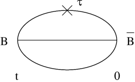
Figure 1: The quark-line connected diagram, left hand picture, and quark-line disconnected diagram, right hand picture. The cross denotes the operator insertion ${\cal O}(\tau)$.

This latter term is numerically extremely difficult to compute, due to ultra-violet fluctuations. However for the CVC this term is in fact constant. This may be easily seen by substituting $\Omega\to\langle B(t)\bar{B}(0)\rangle_{q}$ into the WI, eq. (4). The RHS is then zero and so using the same argument as before the appropriate ratio is constant for all $\tau$. There is thus no contribution to the discontinuity. Indeed on a finite lattice, we would expect this constant to be exponentially small (with exponent proportional to $N_{T}$). Physically there is no quark-line disconnected term because creating a quark-antiquark pair cannot change the charge. Nevertheless with an eye on the computation of the local current it is useful to consider the difference between the $u$ and $d$ operators, ie the non-singlet operator,

$${\cal O}^{(u-d)}\equiv{\cal O}^{(u)}-{\cal O}^{(d)}\,,$$ (9)

in which the quark-line-disconnected terms cancel and so we find

$$R[J^{(u-d)}_{4}(\tau)]=\left\{\begin{array}[]{ll}c_{1}^{(u-d)}&0\leq\tau\leq t\\ c_{2}^{(u-d)}&t\leq\tau\leq N_{T}-1\end{array}\right.\,,$$ (12)

where the discontinuity between the two constants, $\Delta R[J^{(u-d)}_{4}]$, in eq. (12) is given by

$$\Delta R[J^{(u-d)}_{4}]\equiv c_{1}^{(u-d)}-c_{2}^{(u-d)}=\chi^{(u)}-\chi^{(d)}=1\,.$$ (13)

An example for the ratio $R[J^{(u-d)}_{4}]$ is shown in Fig. 2.

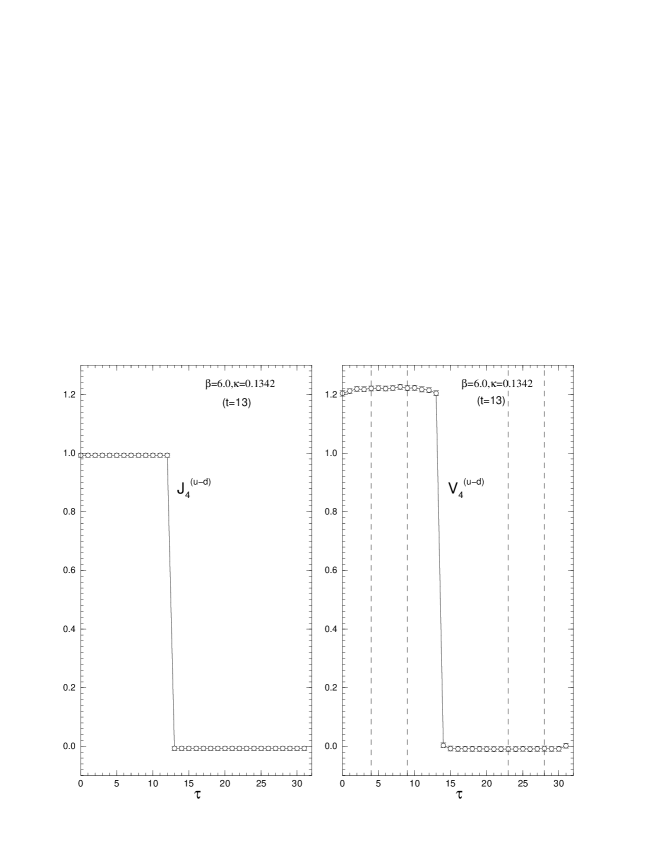
Figure 2: $R[J_{4}^{(u-d)}(\tau)]$ and $R[V_{4}^{(u-d)}(\tau)]$ plotted against the operator position $\tau$ for the quenched ($n_{f}=0$) data set $\beta=6.0$, $\kappa=0.1342$ on an $N_{S}^{3}\times N_{T}=16^{3}\times 32$ lattice with $t=13$. Typical fit intervals for $V_{4}^{(u-d)}$ are given by the pairs of vertical dashed lines. The relationship between $am_{q}$ and $\kappa$ is given in eq. (15).

For $J_{4}^{(u-d)}$ a very good signal is observed. For the jump, as expected, we find $1$ to within machine precision.

The local vector current (LVC) does not obey the WI given in eq. (4), but as $J_{\mu}^{(q)}=V^{(q)}_{\mu}+O(a)$ there is an additional term formally of $O(a)$ on the RHS of this equation. However perturbatively expanding eq. (4) gives loop graphs with ultra-violet divergences $\sim 1/a$ and so this additional term gives a contribution. Thus to obey the WI to $O(a^{2})$, $V_{\mu}$ must be renormalised with renormalisation constant $Z_{V}$ and the quark-line disconnected term in Fig. 1 may give an $O(a)$ contribution. Again to avoid computing this term we consider the non-singlet operator. The necessity for a renormalisation constant is also reflected in the fact that $\Delta R[V_{4}^{(u-d)}]$ will not be equal to one. This is illustrated in the RH picture of Fig. 2. So we can define the renormalisation and improvement constants ($Z_{V}$ and $b_{V}$ respectively) by demanding that the local current has the same behaviour as the conserved current, ie

$$Z_{V}(1+am_{q}b_{V})\equiv\left(\Delta R[V_{4}^{(u-d)}]\right)^{-1}\,.$$ (14)

Thus upon plotting the data for $(\Delta R[V_{4}^{(u-d)}])^{-1}$ against $am_{q}$, we see that the intercept gives $Z_{V}$ while the gradient gives $Z_{V}b_{V}$. Note that $Z_{V}$ has potential $O(a^{2})$ differences to other definitions of the renormalisation constant while $b_{V}$ has possible $O(a)$ differences.

While this procedure is correct in the quenched case, for the unquenched case for complete $O(a)$ cancellation, $g_{0}$ in $Z_{V}$ should be replaced by $\tilde{g}_{0}$ where we have $\tilde{g}_{0}^{2}=g_{0}^{2}(1+b_{g}am_{q})$, [14]. Thus the LHS of eq. (14) should now become $Z_{V}(1+am_{q}(b_{V}+\mbox{\small$\frac{1}{2}$}b_{g}{g_{0}\over Z_{V}}{\partial Z_{V}\over\partial g_{0}}))$. So while the intercept still gives $Z_{V}$, the gradient and hence $b_{V}$ is modified. $b_{g}$ is only known to one loop perturbation theory, $b_{g}=0.01200n_{f}g_{0}^{2}+O(g_{0}^{4})$, [14]. Estimating $\partial Z_{V}/\partial g_{0}$ for unquenched fermions from the Padé fit, eq. (18) and Table 4 to be $\sim-1.3$ gives roughly for the additonal term a decrease of $\sim 0.02$. As numerically $b_{V}$ will turn out to be $\sim 2$, then this could give a $1-2\%$ correction. At present, due to uncertainties in estimating this extra term, we shall ignore this small correction factor.

3 Simulation parameters and raw results for $O(a)$ improved fermions

We have made runs at $\beta=6.0$, $6.2$ and $6.4$ for quenched fermions and $\beta=5.20$, $5.25$ and $5.29$ for unquenched fermions. The run parameters and results for $(\Delta R(V_{4}^{(u-d)}])^{-1}$ are given in Tables 1 and 2.

$\beta$	$c_{sw}$	$\kappa$	$N_{S}^{3}\times N_{T}$	$\#$ configs.	$(\Delta R[V_{4}^{(u-d)}])^{-1}$
6.0	1.769	0.1320	$16^{3}\times 32$	$O(450)$	0.8839(4)
6.0	1.769	0.1324	$16^{3}\times 32$	$O(560)$	0.8717(3)
6.0	1.769	0.1333	$16^{3}\times 32$	$O(560)$	0.8418(4)
6.0	1.769	0.1338	$16^{3}\times 32$	$O(520)$	0.8240(6)
6.0	1.769	0.1342	$16^{3}\times 32$	$O(740)$	0.8124(8)
6.2	1.614	0.1333	$24^{3}\times 48$	$O(300)$	0.8691(2)
6.2	1.614	0.1339	$24^{3}\times 48$	$O(300)$	0.8503(2)
6.2	1.614	0.1344	$24^{3}\times 48$	$O(300)$	0.8342(2)
6.2	1.614	0.1349	$24^{3}\times 48$	$O(470)$	0.8186(2)
6.4	1.526	0.1338	$32^{3}\times 48$	$O(220)$	0.8624(1)
6.4	1.526	0.1342	$32^{3}\times 48$	$O(120)$	0.8504(2)
6.4	1.526	0.1346	$32^{3}\times 48$	$O(220)$	0.8376(1)
6.4	1.526	0.1350	$32^{3}\times 48$	$O(320)$	0.8253(1)
6.4	1.526	0.1353	$32^{3}\times 64$	$O(260)$	0.8163(3)

Table 1: Parameter values used in the quenched simulations with improved fermions, together with $(\Delta R[V_{4}^{(u-d)}])^{-1}$. The fit intervals chosen were $[n_{l},n_{u}]$ and $[N_{T}-n_{l},N_{T}-n_{u}]$ where $[n_{l},n_{u}]=[9,13]$, $[6,11]$, $[7,16]$ for $\beta=6.0$, $6.2$ and $6.4$ respectively.

$\beta$	$c_{sw}$	$\kappa_{sea}$	$N_{S}^{3}\times N_{T}$	$\#$ trajs.	Group	$(\Delta R[V_{4}^{(u-d)}])^{-1}$
5.20	2.0171	0.1342	$16^{3}\times 32$	5000	QCDSF	0.8060(09)
5.20	2.0171	0.1350	$16^{3}\times 32$	8000	UKQCD	0.7731(10)
5.20	2.0171	0.1355	$16^{3}\times 32$	8000	UKQCD	0.7537(16)
5.25	1.9603	0.1346	$16^{3}\times 32$	2000	QCDSF	0.8019(08)
5.25	1.9603	0.1352	$16^{3}\times 32$	8000	UKQCD	0.7781(08)
5.25	1.9603	0.13575	$24^{3}\times 48$	2000	QCDSF	0.7560(06)
5.29	1.9192	0.1340	$16^{3}\times 32$	4000	UKQCD	0.8328(07)
5.29	1.9192	0.1350	$16^{3}\times 32$	5000	QCDSF	0.7948(03)
5.29	1.9192	0.1355	$24^{3}\times 48$	2000	QCDSF	0.7747(04)

Table 2: Data sets used in the unquenched, $n_{f}=2$, simulations together with $(\Delta R[V_{4}^{(u-d)}])^{-1}$. The fit intervals chosen were $[9,13]$ and $[N_{T}-9,N_{T}-13]$.

The bare quark mass is defined as

$$am_{q}(\kappa,g_{0})={1\over 2}\left({1\over\kappa}-{1\over\kappa_{c}(g_{0})}\right)\,,$$ (15)

where $\kappa$ is the hopping parameter of the simulation. It is necessary to find $\kappa_{c}(g_{0})$, ie the critical point where the (bare) quark mass vanishes. From PCAC we know that the quark mass is $\propto m_{ps}^{2}$ and we can use this to determine where the quark mass vanishes. However a more precise/stable determination was often possible if the PCAC quark mass $m_{q}^{\mbox{\tiny$AWI$}}$ was used, so we fitted the dimensionless quantity,

$$X = F(r_{0}m_{q}^{\mbox{\tiny$IMP$}})$$ (16)

$$\equiv B_{1}r_{0}m^{\mbox{\tiny$IMP$}}_{q}+B_{2}(r_{0}m^{\mbox{\tiny$IMP$}}_{q})^{2}+\ldots\,,$$

where $X=r_{0}m_{q}^{\mbox{\tiny$AWI$}}$ and $m^{\mbox{\tiny$IMP$}}_{q}=m_{q}(1+b_{m}am_{q})$ is the $O(a)$ improved quark mass. However determining $am_{q}^{\mbox{\tiny$AWI$}}$ requires a knowledge of the $c_{A}$ improvement coefficent. While this is known for quenched fermions [15] for unquenched fermions this more sensitively affects the value of $am_{q}^{\mbox{\tiny$AWI$}}$. Thus in this case we have set $X=(r_{0}m_{ps})^{2}$. $r_{0}$ in eq. (16) is the ‘force’ scale, [16]. While $r_{0}$ could be omitted for quenched fermions, for unquenched fermions $r_{0}$ becomes quark mass as well as coupling constant dependent and we use the results given in [17], supplemented by [18]. For quenched fermions, we fitted both $B_{1}$ and $B_{2}$ coefficients, which practically meant that no $b_{m}$ coefficient was needed, being absorbed into the $B_{2}$ coefficient, while for unquenched fermions, as we had only three quark mass values we set $B_{2}=0$ and used a tadpole improved value of $b_{m}$, following the prescription given in [10] (and using the plaquette values given in [17]). This gave the results for $\kappa_{c}$ in Table 3.

$\beta$	$\kappa_{c}$	$Z_{V}$	$Z_{V}b_{V}$	$b_{V}$
6.0	0.135201(9)	0.7799(7)	1.168(10)	1.497(13)
6.2	0.135803(3)	0.7907(3)	1.135(06)	1.436(08)
6.4	0.135744(1)	0.8027(2)	1.116(04)	1.391(05)
5.20	0.136072(10)	0.7304(18)	1.472(44)	2.015(61)
5.25	0.136287(09)	0.7349(09)	1.460(31)	1.987(43)
5.29	0.136368(09)	0.7420(07)	1.411(19)	1.902(25)

Table 3: $\kappa_{c}(g_{0})$, the intercept $Z_{V}$, gradient $Z_{V}b_{V}$ and $b_{V}$ for the quenched data sets ($\beta=6.0$, $6.2$ and $6.4$) and for the unquenched data sets ($\beta=5.20$, $5.25$ and $5.29$).

For quenched fermions these numbers are in good agreement with those given in [15].

As discussed in section 2 we now measure the intercept and gradient of $(\Delta R[V_{4}^{(u-d)}])^{-1}$ against $am_{q}$. The results are shown in Fig. 3

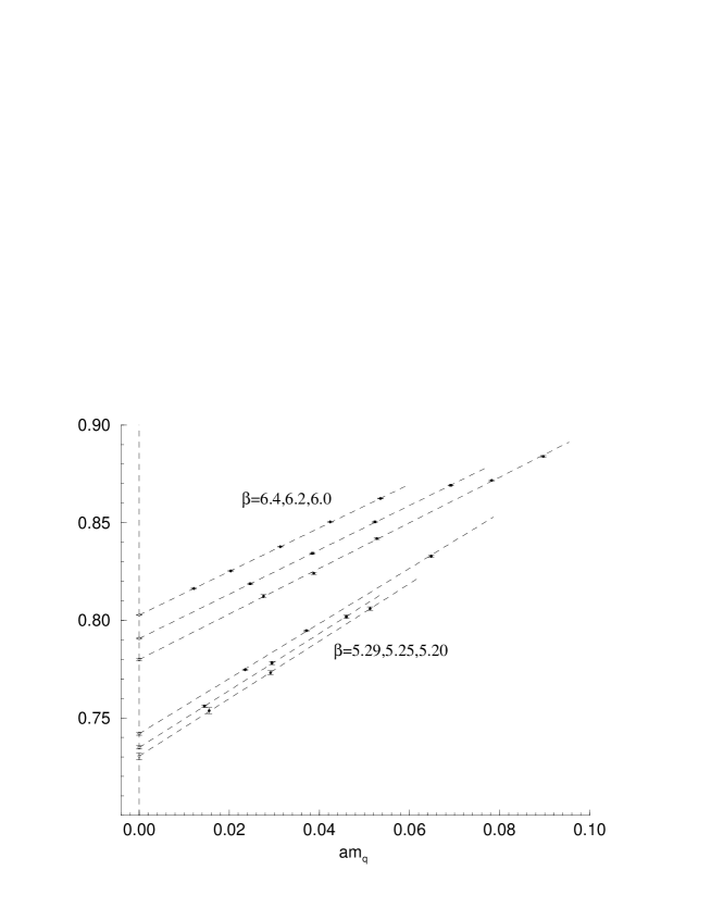
Figure 3: Linear extrapolations for $(\Delta R[V_{4}^{(u-d)}])^{-1}$ for the quenched data at $\beta=6.0$, $6.2$ and $6.4$ (upper set of lines, from $\beta=6.4$, upper line, to $6.0$, lower line) and for the unquenched data at $\beta=5.20$, $5.25$ and $5.29$ (lower set of lines, with the highest being for $\beta=5.29$).

for both the quenched and unquenched data. Very good linearity is seen in the results, which enables a precise estimation of the intercept and slope. The results are also given in Table 3. While these extrapolations have no problems the determination of $\kappa_{c}$ may be more problematic. To give an estimate of possible further errors, if $\kappa_{c}$ is varied by $\delta\kappa_{c}$, then we have

$$\delta Z_{V}\sim b_{V}Z_{V}\delta(am_{q})\,,\quad\delta b_{V}\sim b_{V}^{2}\delta(am_{q})\,,\quad\mbox{with}\quad\delta(am_{q})\sim{1\over 2\kappa_{c}^{2}}\delta\kappa_{c}\,.$$ (17)

For example, taking $\delta\kappa_{c}\sim 0.2\times 10^{-4}$ gives $\delta(am_{q})\sim 0.0005$ and $\delta Z_{V}\sim 0.0006$, $\delta b_{V}\sim 0.001$. These are of the same order or less than the given statistical error.

4 $Z_{V}$ and $b_{V}$ for $O(a)$ improved fermions

We are now in a position to give our final results for $Z_{V}$ and $b_{V}$. From eq. (14), dividing the gradient in Fig. 3 by the intercept gives in Table 3 in the third and fifth columns $Z_{V}$ and $b_{V}$ respectively.

As for both quenched and unquenched fermions we have three $\beta$ values, we can attempt to make a Padé-type fit of the form

$$P(g_{0})={1+p_{1}g_{0}^{2}+p_{2}g_{0}^{4}\over 1+q_{1}g_{0}^{2}}\,,$$ (18)

for $Z_{V}(g_{0})$, $b_{V}(g_{0})$ constrained to reproduce the weak coupling results, eqs. (1), (2). There are thus $2$ free parameters. In Table 4

	$p_{1}$	$p_{2}$	$q_{1}$
Quenched ($n_{f}=0$)
$Z_{V}$	-0.634	0.0196	-0.504
$b_{V}$	-0.627	-0.0444	-0.781
Unquenched ($n_{f}=2$)
$Z_{V}$	-0.796	0.0652	-0.667
$b_{V}$	-0.614	-0.0432	-0.767

Table 4: The Padé fit results as defined in eq. (18).

we give the results of the fits. Note however that even though we have matched to the weak coupling results, as the range of $\beta$ where the numerical results lie is rather small and far away from this region, intermediate regions may not be represented so well. We estimate total errors on these Padé results to be about $\mbox{\small$\frac{1}{2}$}\%$ for $Z_{V}$ for both the quenched and unquenched cases and for $b_{V}$, $1\%$ and $2\%$ for quenched and unquenched fermions respectively. (Note also that for the unquenched results there is a further error in $b_{V}$ of $1-2\%$ due to an uncertainty in $b_{g}$ as discussed previously in section 2.)

Alternative non-perturbative determinations for quenched $O(a)$ improved fermions have been given by the ALPHA Collaboration, using the Schrödinger functional method, [19], the LANL Collaboration, [20, 21] using other Ward identities and the SPQcdR Collaboration [22] using the RI-MOM scheme, [23]. All these other methods have reasonable agreement with the results given here, as can be seen in the following pictures. (One should remember that $Z_{V}$ definitions in particular RI-MOM can vary by at least $O(a^{2})$ and $b_{V}$ definitions can vary by $O(a)$.) In Figs. 4, 5

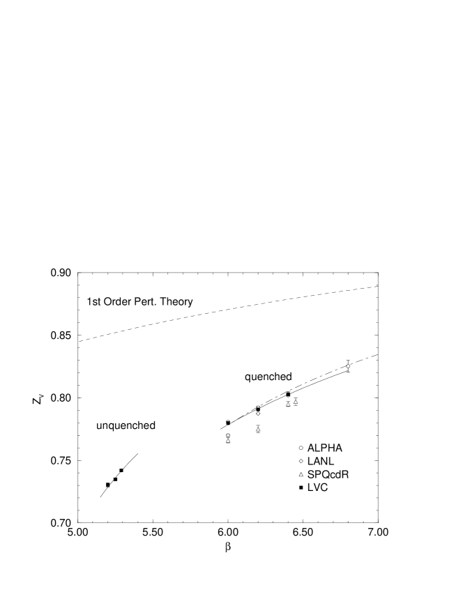
Figure 4: $Z_{V}$ (LVC, filled squares) determined in this work for quenched and unquenched $O(a)$ improved fermions. For quenched fermions a comparison is made with ALPHA, [19], LANL, [21] and SPQcdR, [22]. Padé fits are also given for our (full lines) and the ALPHA (dot-dashed line) results. The dashed line is the first order perturbative result, eq. (1).

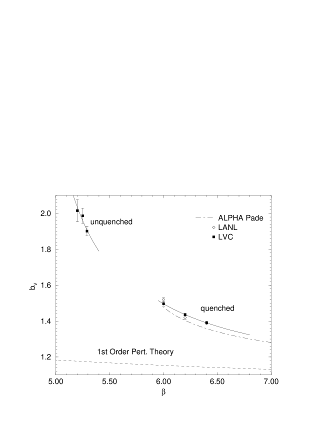
Figure 5: $b_{V}$ (LVC, filled squares) determined in this work for both quenched and unquenched $O(a)$ improved fermions. Also shown are our Padé fits (full lines) and that from ALPHA, [19] (dot-dashed line), and the LANL, [21] results for quenched fermions. The dashed line is the first order perturbative result, eq. (2).

we plot our results for $Z_{V}$ and $b_{V}$ respectively for both quenched and unquenched fermions. As, in particular for unquenched fermions the available $\beta$-range is rather narrow and far from the continuum limit the Padé extrapolation should be treated with some caution. However it is encouraging to note that the ordering of the points is correct. Thus the Padé results should be regarded mainly as an interpolating formula between the various $\beta$ values. Note however in the quenched case that the Padé results track quite well the ALPHA results.

Some of our earlier results for $Z_{V}$ for quenched fermions can be found in [24]. Note also an example of the large increase in the statistical fluctuations shown there when matrix elements with moving nucleons ($\vec{p}\not=\vec{0}$) are considered.

5 $Z_{V}$ for unimproved fermions

Although most of our results are for $O(a)$ improved fermions we also have results at $\beta=6.0$ for quenched unimproved fermions ($c_{sw}=0$) which serve as a useful check on the improved results. The method is identical to that described previously, so we shall just give the results here. In Table 5

$\beta$	$\kappa$	$N_{S}^{3}\times N_{T}$	$\#$ configs.	$(\Delta R[V_{4}^{(u-d)}])^{-1}$
6.0	0.1515	$16^{3}\times 32$	$O(980)$	0.7521(2)
6.0	0.1530	$16^{3}\times 32$	$O(1130)$	0.7220(2)
6.0	0.1550	$16^{3}\times 32$	$O(1360)$	0.6845(3)
6.0	0.1550	$24^{3}\times 32$	$O(220)$	0.6837(3)
6.0	0.1558	$24^{3}\times 32$	$O(220)$	0.6689(4)
6.0	0.1563	$24^{3}\times 32$	$O(220)$	0.6595(6)
6.0	0.1563	$32^{3}\times 48$	$O(250)$	0.6599(4)
6.0	0.1566	$32^{3}\times 48$	$O(410)$	0.6545(5)

Table 5: Parameter values used in the quenched simulations with unimproved fermions, together with $(\Delta R[V_{4}^{(u-d)}])^{-1}$.

we give the parameters of the runs and raw results. Note that the range of quark masses is greater than in the $O(a)$ improved case and that we have runs on different volumes at the same quark mass. It is apparent from the table that finite volume effects are rather small.

Plotting $(\Delta R[V_{4}^{(u-d)}])^{-1}$ against $am_{q}$ gives the result $Z_{V}=0.6436(3)$ at $\beta=6.0$ (for completeness the gradient is $0.9088(27)$), using $\kappa_{c}=0.157129(10)$. We see that the numerical value is somewhat lower than the equivalent $O(a)$ improved value. This result is consistent, but a little larger than the recent determination given in [25] (although there different $\beta$-values are used). Again this is not unexpected, as different determinations of $Z_{V}$ can now differ by $O(a)$ terms (see also [24]).

6 Conclusions

Our method is not in disagreement with results of other approaches for $O(a)$ improved quenched fermions. For example even for $b_{V}$ there is only a few percent scatter in comparison with other methods. This is what one would expect with $O(a)$ discrepancy between the various definitions.

$Z_{V}$ and $b_{V}$ are both further away from $1$ in the unquenched case than in the quenched case at comparable lattice spacings (roughly $a_{n_{f}=2}(5.25)\sim a_{n_{f}=0}(6.0)$). This is partially an effect from the use of (numerically) smaller $\beta$ factors and also partially because of the presence of fermions which induces a shift in the effective $\beta$. Finally we note that we cannot use one loop perturbation expansion results in the present day quenched/unquenched $\beta$ regions, although this can be improved by using TI-RGI-BPT, eg [26], or BLM/TI methods, [27].

Appendix

The result in eq. (8) may alternatively be shown using transfer matrix methods. As $J^{(q)}_{4}$ is conserved then (with normalisation $\langle i|j\rangle=\delta_{ij}$)

$$\langle i|J^{(q)}_{4}|j\rangle=\chi_{i}^{(q)}\delta_{ij}\,,$$ (19)

where $\chi_{i}^{(q)}$ is the ‘charge’ (associated with the current $J^{(q)}_{\mu}$) of the state $|i\rangle$. Thus inserting complete sets of states into the three-point function gives

$$\langle B(t)J^{(q)}_{4}(\tau)\bar{B}(0)\rangle = \sum_{ij}\langle j|B|i\rangle\chi_{i}^{(q)}\langle i|\bar{B}|j\rangle e^{-aE_{i}t}e^{-aE_{j}(N_{T}-t)}\qquad 0<\tau<t$$ (20)

$$= \langle 0|B|N\rangle\chi^{(q)}_{N}\langle N|\bar{B}|0\rangle e^{-am_{N}t}+\ldots\,,$$

(where the second equation assumes that the excited states have died away and takes the charge on the nucleon, $\chi^{(q)}_{N}$, to be $\chi^{(q)}_{N}=\langle N|J^{(q)}_{4}|N\rangle$) and similarly

$$\langle J^{(q)}_{4}(\tau)B(t)\bar{B}(0)\rangle = \sum_{ij}\chi^{(q)}_{j}\langle j|B|i\rangle\langle i|\bar{B}|j\rangle e^{-aE_{i}t}e^{-aE_{j}(N_{T}-t)}\qquad t<\tau<N_{T}$$ (21)

$$= \chi^{(q)}_{N^{*}}\langle\bar{N}^{*}|B|0\rangle\langle 0|\bar{B}|\bar{N}^{*}\rangle e^{-am_{N^{*}}(N_{T}-t)}+\ldots\,,$$

$N^{*}$ being the parity partner of the nucleon and where $\chi^{(q)}_{N^{*}}=\langle\bar{N}^{*}|J^{(q)}_{4}|\bar{N}^{*}\rangle\equiv-\chi^{(q)}_{N}$. All of these expressions are independent of $\tau$. The transfer matrix approach thus again predicts perfect plateaus for $J^{(q)}_{4}$. Furthermore, the discontinuity is given by the difference between these two expressions. As $\langle i|\bar{B}|j\rangle$ is only non-zero if the difference in the charges of $|i\rangle$ and $|j\rangle$ is equal to that of the charge of a nucleon, then we can replace $\chi^{(q)}_{i}-\chi^{(q)}_{j}$ by $\chi^{(q)}_{N}$ to give

$$\langle B(t)J^{(q)}_{4}(\tau)\bar{B}(0)\left.\rangle\right|_{0<\tau<t}-\langle J^{(q)}_{4}(\tau)B(t)\bar{B}(0)\left.\rangle\right|_{t<\tau<N_{T}}$$ (22)

$$= \sum_{ij}(\chi^{(q)}_{i}-\chi^{(q)}_{j})\langle j|B|i\rangle\langle i|\bar{B}|j\rangle e^{-aE_{i}t}e^{-aE_{j}(N_{T}-t)}$$

$$= \chi^{(q)}_{N}\langle B(t)\bar{B}(0)\rangle\,.$$

From eqs. (20), (21) we see that for $t<N_{T}/2$ (the case considered here) the exponential factor is larger for the term $0<\tau<t$ which means that $c^{(q)}_{2}$ is small in comparison with $c^{(q)}_{1}$.

References

- [1] K. G. Wilson, in New Phenomena in Subnuclear Physics, ed. A. Zichichi (Plenum Press, New York) Part A (1975) 69.
- [2] M. Lüscher, Lectures given at the Les Houches Summer School “Probing the Standard Model of Particle Interactions”, July 1997, hep-lat/9802029.
- [3] R. Sommer, Lectures given at the 36th Internationale Universitätswochen für Kernphysik und Teilchenphysik, Schladming, Austria, March 1997, hep-ph/9711243.
- [4] A. S. Kronfeld, At the Frontiers of Physics: Handbook of QCD, Vol. 4, edited by M. Shifman (World Scientific, Singapore, 2002), hep-lat/0205021.
- [5] F. Niedermayer, Nucl. Phys. B(Proc. Suppl.) 73 (1999) 105, hep-lat/9810026.
- [6] S. Capitani, M. Göckeler, R. Horsley, P. E. L. Rakow and G. Schierholz, Phys. Lett. B468 (1999) 150, hep-lat/9908029.
- [7] E. Gabrielli, G. Martinelli, C. Pittori, G. Heatlie and C. T. Sachrajda, Nucl. Phys. B362 (1991) 475.
- [8] M. Göckeler, R. Horsley, E.-M. Ilgenfritz, H. Oelrich, H. Perlt, P. Rakow, G. Schierholz, A. Schiller and P. Stephenson, Nucl. Phys. B(Proc. Suppl.) 53 (1997) 896, hep-lat/9608033.
- [9] S. Sint and P. Weisz, Nucl. Phys. B502 (1997) 251, hep-lat/9704001.
- [10] S. Capitani, M. Göckeler, R. Horsley, H. Perlt, P. E. L. Rakow, G. Schierholz and A. Schiller, Nucl. Phys. B593 (2001) 183, hep-lat/0007004.
- [11] T. Bakeyev, M. Göckeler, R. Horsley, D. Pleiter, P. E. L. Rakow, A. Schäfer, G. Schierholz and H. Stüben, Nucl. Phys. B(Proc. Suppl.) 119 (2003) 467, hep-lat/0209148.
- [12] M. Göckeler, R. Horsley, E.-M. Ilgenfritz, H. Perlt, P. Rakow, G. Schierholz and A. Schiller, Phys. Rev. D53 (1996) 2317, hep-lat/9508004.
- [13] M. Göckeler, R. Horsley, M. Ilgenfritz, H. Perlt, P. Rakow, G. Schierholz and A. Schiller, Nucl. Phys. B(Proc. Suppl.) 42 (1995) 337, hep-lat/9412055.
- [14] M. Lüscher, S. Sint, R. Sommer and P. Weisz, Nucl. Phys. B478 (1996) 365, hep-lat/9605038.
- [15] M. Lüscher, S. Sint, R. Sommer, P. Weisz and U. Wolff, Nucl. Phys. B491 (1997) 323, hep-lat/9609035.
- [16] R. Sommer, Nucl. Phys. B411 (1994) 839, hep-lat/9310022.
- [17] S. Booth, M. Göckeler, R. Horsley, A. C. Irving, B. Joo, S. Pickles, D. Pleiter, P. E. L. Rakow, G. Schierholz, Z. Sroczynski and H. Stüben, Phys. Lett. B519 (2001) 229, hep-lat/0103023.
- [18] A. Irving, unpublished.
- [19] M. Lüscher, S. Sint, R. Sommer and H. Wittig, Nucl. Phys. B491 (1997) 344, hep-lat/9611015.
- [20] T. Bhattacharya, R. Gupta, W. Lee and S. Sharpe, Phys. Rev. D63 (2001) 074505, hep-lat/0009038.
- [21] T. Bhattacharya, R. Gupta, W. Lee and S. Sharpe, Nucl. Phys. B(Proc. Suppl.) 106 (2002) 789, hep-lat/0111001.
- [22] D. Becirevic, V. Gimenez, V. Lubicz, G. Martinelli, M. Papinutto, J. Reyes and C. Tarantino, Nucl. Phys. B(Proc. Suppl.) 119 (2003) 442, hep-lat/0209168.
- [23] G. Martinelli, C. Pittori, C. T. Sachrajda, M. Testa and A. Vladikas, Nucl. Phys. B445 (1995) 81, hep-lat/9411010.
- [24] S. Capitani, M. Göckeler, R. Horsley, B. Klaus, H. Oelrich, H. Perlt, D. Petters, D. Pleiter, P. Rakow, G. Schierholz, A. Schiller and P. Stephenson, 31st Ahrenshoop Symposium on the Theory of Elementary Particles, (Buckow, Germany, September 1997), editors H. Dorn, D. Lüst and G. Weigt, Wiley-VCH, hep-lat/9801034.
- [25] S. Aoki, G. Boyd, R. Burkhalter, S. Ejiri, M. Fukugita, S. Hashimoto, Y. Iwasaki, K. Kanaya, T. Kaneko, Y. Kuramashi, K. Nagai, M. Okawa, H. P. Shanahan, A. Ukawa and T. Yoshie, Phys. Rev. D67 (2003) 034503, hep-lat/0206009.
- [26] S. Capitani, M. Göckeler, R. Horsley, D. Pleiter, P. Rakow, H. Stüben and G. Schierholz, Nucl. Phys. B(Proc. Suppl.) 106 (2002) 299, hep-lat/0111012.
- [27] J. Harada, S. Hashimoto, A. S. Kronfeld and T. Onogi, Phys. Rev. D67 (2003) 014503, hep-lat/0208004.