Advanced Algorithms for the Simulation of Gauge Theories with Dynamical Fermionic Degrees of Freedom

Abstract

The topic of this thesis is the numerical simulation of quantum chromodynamics including dynamical fermions. Two major problems of most simulation algorithms that deal with dynamical fermions are (i) their restriction to only two mass-degenerate quarks, and (ii) their limitation to relatively heavy masses. Realistic simulations of quantum chromodynamics, however, require the inclusion of three light dynamical fermion flavors. It is therefore highly important to develop algorithms which are efficient in this situation.

This thesis is focused on the implementation and the application of a novel kind of algorithm which is expected to overcome the limitations of older schemes. This new algorithm is named Multiboson Method. It allows to simulate an arbitrary number of dynamical fermion flavors, which can in principle have different masses. It will be shown that it exhibits better scaling properties for light fermions than other methods. Therefore, it has the potential to become the method of choice.

An explorative investigation of the parameter space of quantum chromodynamics with three flavors finishes this work. The results may serve as a starting point for future realistic simulations.

Chapter 0 Introduction

The works of the LORD are great,
sought out by all them
that have pleasure in them.
Psalm 111, Verse 2.

Throughout history one of the fundamental driving forces of man has been the desire to understand nature. In the past few centuries, natural sciences have paved the way to several revolutionary insights to the structures underlying our world. Some of them founded fundamental benefits for the quality of life and the advance of civilization. In particular, in the recent decades, computer technology has set the base for a major leap of several important facets of human existence.

A major challenge is posed by fundamental research, which does not directly aim towards developing industrial applications, but instead examines structures and relations relevant for future technologies. The goal of fundamental research is to formulate theories which comprise as many different phenomena as possible and which are, at the same time, as simple as they can be.

The branch of natural sciences which concentrates on the structures underlying matter and energy is termed particle physics. This field lives on contributions from experiments, providing insights of how the particles which constitute our world interact. A further driving force behind particle physics is the desire to find a simple description of the mechanisms underlying these experiments. The field of particle physics has benefitted from the evolution in computer science, but on the other hand theoretical physicists have triggered many pivotal developments in technology we have today.

Current physical theories categorize the interactions between matter and energy into four different types of fundamental forces. These forces are gravitation, electromagnetism, and finally the weak and the strong interactions. The strong interaction is responsible for the forces acting between hadrons, i.e. between neutrons, protons and nuclei built up from these particles. Its name originates from the fact that it is the strongest among the other forces on the energy scale of hadronic interactions. The strengths of the four forces can be stated in terms of their coupling constants [1]:

$$\alpha_{\mbox{\tiny em}}(Q^{2}=0) \sim 1/137.035\,999\,76(50)\,,$$

$$\alpha_{\mbox{\tiny strong}}(Q^{2}=m_{Z}^{2}) \sim 0.1185(20)\,,$$

$$G_{\mbox{\tiny weak}} \sim 1.166\,39(1)\times 10^{-5}\,\mbox{GeV}^{-2}\,,$$

$$G_{\mbox{\tiny Newton}} \sim 6.707(10)\times 10^{-39}\,\mbox{GeV}^{-2}\,.$$ (1)

It is apparent, that gravitation is many orders of magnitude weaker than the other forces and thus is expected to play no role on the energy scales important for particle physics so far [2].

In contrast to electromagnetic interactions and gravity, strong and weak forces do not have infinite ranges. They exhibit finite ranges up to at most the size of a nucleus. Thus, they only play a role in nuclear interactions, but are almost completely negligible on the level of atoms and molecules. Any particular process can be dissected into a multitude of processes acting at a smaller scale. Hence, a process with a given action $S\{\mbox{Process}\}$ may be described by a set of subprocesses $\sum_{i}S\{\mbox{Subprocess}_{i}\}$ with smaller actions $S\{\mbox{Subprocess}_{i}\}<S\{\mbox{Process}\}$. We can tell from observations that processes are essentially deterministic if the action of the process in question $S\{\mbox{Process}\}$ is far larger than some action $\hbar$ which is known as “Planck’s constant” [3]. However, if the action of the process is of the order of $\hbar$, then the system cannot be described by a deterministic theory any longer and a non-deterministic theory known as quantum mechanics must be employed. Today, all interactions can be described within a quantum-mechanical framework, with the exception of gravity, which has so far not been successfully formulated as a consistent quantum theory. For a discussion of these topics the reader may consult [4] and references therein.

A necessary requirement for the above iteration to make sense is that it must be possible to recover a classical (non-probabilistic) theory in a certain limit (naturally the $\hbar\to 0$ limit) from a quantum theory. This limit is given by the WKB approximation [5]. One finds that an expansion exists, where the amplitude of a process can be formulated as a power-series in $\hbar$:

$$A\{\mbox{Process}\}=A\{\mbox{Classical}\}+\hbar A_{1}+\hbar^{2}A_{2}+\cdots\;.$$ (2)

In the limit $\hbar\to 0$ the classical amplitude is recovered. But Eq. (2) also shows that the quantum theory contains more information than the classical theory: Different choices for the series coefficients $\{A_{1},A_{2},\dots\}$ obviously lead to the same classical theory. Thus, if one intends to construct a quantum theory starting from the classical theory, there is always an ambiguity of how to proceed [5]. The correct prescription can only be found by experimental means.

There exist several quantization prescriptions to build a quantum theory. All of these have in common that they describe a system which exhibits a probabilistic interpretation of physical observables and a deterministic evolution equation of some underlying degrees of freedom. The quantum theory which is believed to constitute the correct quantum theory of the strong interaction is called quantum chromodynamics (QCD).

In general, a quantum mechanical system can not be solved exactly, but only by use of certain approximations. The approximation most commonly employed is known as perturbation theory and is applicable in a large variety of cases. It is known to fail, however, when applied to the low-energy regime of QCD, where a diversity of interesting phenomena occurs. Hence, different techniques commonly called “non-perturbative” methods must be employed. One of these non-perturbative methods is the simulation of the system in a large-scale numerical calculation, an approach which is referred to as “Lattice QCD”. This approach is in the focus of this thesis.

When performing numerical simulations within Lattice QCD, one finds that the simulation of the bosonic constituents of QCD, the “gluons”, stand at the basis of research efforts, see [6] for a pioneering publication.

The inclusion of dynamical fermions poses a serious problem. Although it has become clear in [7, 8] that without dynamical fermions the low-energy hadron spectrum is reproduced with $10\%$ accuracy, several important aspects of low-energy QCD require the inclusion of dynamical fermions. One case where the inclusion of dynamical fermions is phenomenologically vital is given by the mass of the $\eta^{\prime}$ meson, cf. [9].

The numerical simulation of dynamical fermions is plagued by severe difficulties. In particular, the requirement that the fermions must be light is to be met, since only in this case the chiral behavior of QCD, i.e. the behavior at light fermion masses, is reproduced correctly. But in this particular limit, the algorithms suffer from a phenomenon known as critical slowing down, i.e. a polynomial decrease in efficiency as the chiral point is approached.

Furthermore, the majority of algorithms in use today can only treat two mass-degenerate dynamical fermion flavors, a situation not present in strong interactions as observed in nature. In fact, one has to use three dynamical fermion flavors [10].

Thus, the demands on an algorithm for the simulation of dynamical fermion flavors must consist of (i) the suitability for the simulation of three dynamical fermion flavors, and (ii) the efficiency of the algorithm with regard to critical slowing down. These two requirements are not met by the commonly used algorithm in Lattice QCD, the hybrid Monte-Carlo (HMC) algorithm.

The topic of this thesis is the exploration of a new type of algorithm, known as the multiboson algorithm. This algorithm is expected to be superior to the HMC algorithm with regard to the above properties. In particular, it will be examined how to tune and optimize this class of algorithms and if these algorithms are suitable for the simulation of three light, dynamical, and mass-degenerate fermion flavors.

The thesis is organized as follows: the theoretical background of the strong interaction, the quantization of field theories, and the definition of lattice gauge theories is given in chapter 1. The tools required to perform numerical simulations in lattice theories and the analysis of time series are formulated in chapter 2. The optimization and tuning of the algorithm is discussed in chapter 3.

A direct comparison of the multiboson algorithm with the hybrid Monte-Carlo method is performed in chapter 4. In particular, the scaling of the algorithms with the quark mass has been focused at.

A particularly useful application of the multiboson algorithm appears to be the simulation of QCD with three dynamical fermion flavors. Such a simulation allows to assess the suitability of multiboson algorithms for future simulations aimed at obtaining physically relevant results. A first, explorative investigation of the parameter space which might be relevant for future simulations is presented in chapter 5.

Finally the conclusions are summarized in chapter 6.

Appendix 7 contains a short overview of the notation used in this thesis. An introduction to group theory and the corresponding algebras is given in App. 8. The explicit expressions used for the local actions required for the implementation of multiboson algorithms are listed in App. 9. At last, App. 10 explains the concepts required for running large production runs, where a huge amount of data is typically generated.

I have to thank many colleagues and friends who have accompanied me during the completion of this thesis and my scientific work. I am indebted to my parents, Astrid Börger, Claus Gebert, Ivan Hip, Boris Postler, and Zbygniew Sroczynski for the time they invested to proof-read my thesis. For the interesting scientific collaborations and many useful discussions I express my gratitude to Guido Arnold, Sabrina Casanova, Massimo D’Elia, Norbert Eicker, Federico Farchioni, Philippe de Forcrand, Christoph Gattringer, Rainer Jacob, Peter Kroll, Thomas Moschny, Hartmut Neff, Boris Orth, Pavel Pobylitza, Nicos Stefanis, and in particular to István Montvay, Thomas Lippert, and Klaus Schilling.

Chapter 1 Quantum Field Theories and Hadronic Physics

This chapter provides a general introduction into the topic of particle physics. It covers both the phenomenological aspects, the mathematical structures commonly used to describe these systems, and the particular methods to obtain results from the basic principles.

Section 1 gives a general overview of the phenomenology of the strong interaction without making direct reference to a particular model.

A short overview of classical (i.e. non-quantum) field theories is given in Sec. 2. With this basis, the general principles of constructing a quantum field theory starting from a classical field theory are presented in Sec. 3. The case of non-relativistic theories is covered in Sec. 1, while the generalization to relativistic quantum field theories requires far more effort. This is described in Sec. 2, where the basic axiomatic frameworks of relativistic quantum field theories are stated.

Particular emphasis will be placed on the path integral quantization which allows for a rigorous and efficient construction of a quantum theory. Section 3 provides a detailed treatise of this method and also contains a discussion of how one can perform computations in practice. An important tool for the evaluation of path integrals is the concept of ensembles, which is introduced in Sec. 4. It will turn out to be essential in numerical simulations of quantum field theories.

Section 4 introduces an important class of quantum field theories, namely the class of gauge theories. These models will be of central importance in the following.

With all necessary tools prepared, Sec. 5 will introduce a gauge theory which is expected to be able to describe the whole phenomenology of the strong interaction. This theory is known as quantum chromodynamics (QCD) and it is the main scope of this thesis. After a general introduction to the properties of QCD in Sec. 1, a method known as factorization is discussed in Sec. 2. This method allows to combine information from the different energy scales and thus provides an essential tool for actual predictions in QCD calculations. Finally, the method of Lattice QCD is discussed in Sec. 3. Lattice simulations exploit numerical integration schemes to gain information about the structure of QCD, and represent the major tool for the purposes of this thesis.

The construction of a quantum field theory based on path integrals requires a certain discretization scheme. This scheme is particularly important in lattice simulations. Therefore, Sec. 6 covers the common discretizations for the different types of fields one encounters in quantum field theories. The case of scalar fields allows for a simple and efficient construction as will be shown in Sec. 1. The case of gauge fields is more involved since there exist several proposals how this implementation should be done. Contemporary simulations focus mainly on the Wilson discretization, although recently a new and probably superior method has been proposed. This method, known as D-theory, is reviewed in Sec. 3.

The discretization of fermion fields is even more involved. The necessary conditions such a scheme has to fulfill are given in Sec. 4 and the scheme used in this thesis, namely the Wilson-fermion scheme, is constructed. In contrast to the cases of scalar and gauge fields, a large number of different fermion discretization schemes are used in actual simulations today, and each has its particular advantages and disadvantages.

This chapter is concluded by the application of the previously discussed discretization schemes to a gauge theory containing both fermions and gauge fields in Sec. 5. Such a model is expected to be the lattice version of gauge theories with fermions, and in particular of QCD.

1 Phenomenology of Strong Interactions

Until 1932 only the electron $e$, the photon $\gamma$ and the proton $p$ have been known as elementary particles (for overviews of the history of particles physics see [11, 12, 13]). The only strong process known was the $\alpha$-decay of a nucleus. The milestones in this period were the detection of the neutron by Chadwick in 1932 and the prediction of the $\pi$-meson (today it is customary to call it simply “pion”) by Yukawa in 1935 as the mediator of the strong force. However, it took until 1948 before the charged pion was actually detected by Lattes. In 1947 particles carrying a new type of quantum number called “strangeness” have been detected by Rochester. In 1950 the neutral pion was detected by Carlson and Bjorkland. It was soon realized that the hadrons were not point-like objects like the leptons, but had an internal structure and accordingly a finite spatial extent.

The experiments to observe the structure of hadrons usually consist of scattering two incoming particles off each other, producing several outgoing particles of possibly different type. If one considers a particular subset of processes where all outgoing particles are of a determined type, one speaks of exclusive reactions. A sub-class of exclusive reactions are the elastic scattering processes, where the incoming and outgoing particles are identical.

The inclusive reactions are obtained by summing over all possible exclusive reactions for given incoming particles. Inclusive electron-nucleon scattering at very large energies is called deep-inelastic scattering (DIS) and played an important role in the understanding of the structure of hadrons. The prediction of scaling by Bjorken in 1969 was confirmed experimentally and led to the insight that the hadrons consist of point-like sub-particles. In 1968 Feynman proposed a model which exhibited this feature, the parton model.

A collection of hadrons, as known in the early 60’s, is given in Tab. 1 together with their properties in the form of quantum numbers. These quantum numbers are known as spin, parity, electric charge $Q$, baryon number $\mathcal{B}$, and strangeness $S$. They are conserved by the strong interaction.

Hadron	Spin${}^{\mbox{\bf Parity}}$	$\mathbf{Q}$	$\mathbf{\cal B}$	$\mathbf{S}$	$\mathbf{m/}$MeV
$\pi^{\pm}$	$0^{-}$	$\pm 1$	$0$	$0$	$140$
$\pi^{0}$	$0^{-}$	$0$	$0$	$0$	$135$
$K^{0}$	$0^{-}$	$0$	$0$	$+1$	$498$
$\bar{K}^{0}$	$0^{-}$	$0$	$0$	$-1$	$498$
$K^{\pm}$	$0^{-}$	$\pm 1$	$0$	$\pm 1$	$494$
$\eta$	$0^{-}$	$0$	$0$	$0$	$547$
$\eta^{\prime}$	$0^{-}$	$0$	$0$	$0$	$958$
$\rho^{\pm}$	$1^{-}$	$\pm 1$	$0$	$0$	$767$
$\rho^{0}$	$1^{-}$	$0$	$0$	$0$	$769$
$K^{*0}$	$1^{-}$	$0$	$0$	$+1$	$896$
$\bar{K}^{*0}$	$1^{-}$	$0$	$0$	$-1$	$896$
$K^{*\pm}$	$1^{-}$	$\pm 1$	$0$	$\pm 1$	$892$
$\omega$	$1^{-}$	$0$	$0$	$0$	$783$
$\phi$	$1^{-}$	$0$	$0$	$0$	$1019$
$p$	$1/2^{+}$	$+1$	$+1$	$0$	$938$
$n$	$1/2^{+}$	$0$	$+1$	$0$	$940$
$\Sigma^{+}$	$1/2^{+}$	$+1$	$+1$	$-1$	$1189$
$\Sigma^{-}$	$1/2^{+}$	$-1$	$+1$	$-1$	$1197$
$\Sigma^{0}$	$1/2^{+}$	$0$	$+1$	$-1$	$1193$
$\Lambda$	$1/2^{+}$	$0$	$+1$	$-1$	$1116$
$\Xi^{0}$	$1/2^{+}$	$0$	$+1$	$-2$	$1315$
$\Xi^{-}$	$1/2^{+}$	$-1$	$+1$	$-2$	$1321$

Table 1: List of selected hadrons with their quantum numbers and their masses in MeV.

The particles may be divided into several groups according to their spin and parity: the particles with even spin are called mesons and the particles with odd spin baryons. Because of their parity and spin, the particles $\pi^{0}$, $\pi^{\pm}$, $K^{\pm}$, $K^{0}$, $\bar{K}^{0}$, $\eta$ and $\eta^{{}^{\prime}}$ are usually called “pseudoscalar mesons”. Similarly, the particles $\rho^{0}$, $\rho^{\pm}$, $\omega$, $K^{*0}$, $K^{*\pm}$, $\bar{K}^{*0}$ and $\varphi$ are named “vector mesons”. The group $p$, $n$, $\Lambda$, $\Sigma^{0}$, $\Sigma^{\pm}$, $\Xi^{-}$ and $\Xi^{0}$ is simply called “baryons”. In each group, the members have roughly similar masses (with the exception of the $\eta^{{}^{\prime}}$ in the group of the pseudoscalar mesons).

In 1963 Gell-Mann and Zweig independently proposed a scheme to classify the known particles as multiplets of the Lie group SU$(3)_{F}$. It turned out that the classification is indeed possible with the exception that there were no particles corresponding to the fundamental triplets of the group. This would imply that the corresponding particles carry fractional charges; particles with such a property have never been seen in any experiment. However, experiments at SLAC in 1971 involving neutrino-nucleon scattering clearly indicated that the data could be accounted for if the parton inside the nucleon had the properties of the particles in the fundamental triplet of the SU$(3)_{F}$ group. This led finally to the identification of the (charged) partons from Feynman’s model with the particles from the classification scheme of Gell-Mann and Zweig. These particles are known today as quarks.

Today a huge number of particles subject to the strong interaction is known from different kinds of experiments. For a complete overview see [1]. To classify them the quark model had to be extended to six kinds of quarks. They are referred to as having “different flavors”, which are new quantum numbers. Thus, they are conserved by the strong interaction. The quarks cover a huge range of masses. Their properties are listed in Tab. 2.

	$\mathbf{Y}$	$\mathbf{T_{3}}$	$\mathbf{Q}$	$\mathbf{\cal B}$	$\mathbf{S}$	$\mathbf{C}$	$\mathbf{B}$	$\mathbf{T}$	$\mathbf{m/\mbox{MeV}}$
$u$	$1/2$	$1/2$	$2/3$	$1/3$	$0$	$0$	$0$	$0$	$1-5$
$c$	$0$	$0$	$2/3$	$1/3$	$0$	$1$	$0$	$0$	$1150-1350$
$t$	$0$	$0$	$2/3$	$1/3$	$0$	$0$	$0$	$1$	$174300\pm 5100$
$d$	$1/2$	$-1/2$	$-1/3$	$1/3$	$0$	$0$	$0$	$0$	$3-9$
$s$	$0$	$0$	$-1/3$	$1/3$	$-1$	$0$	$0$	$0$	$75-170$
$b$	$0$	$0$	$-1/3$	$1/3$	$0$	$0$	$-1$	$0$	$4000-4400$

Table 2: Different flavors of quarks together with their associated quantum numbers.

To classify the multiplets of the flavor group SU$(3)_{F}$, two numbers are required which are usually called $Y$ (the strong hyper-charge) and $T_{3}$ (the isospin). They are defined by

$$Y=S+B,$$

and

$$T_{3}=Q-\frac{1}{2}\left(S+B\right).$$

The three light quarks together with the corresponding anti-particles are shown in Fig. 1. The classifications for the pseudoscalar mesons, the vector mesons and the baryons are given in Figs. 2, 3, and 4.

Figure 1: Fundamental representations of the SU$(3)_{F}$ flavor group. The left graph shows the quark triplet ($u$,$d$,$s$) and the right graph shows the anti-quark triplet ($\bar{u}$,$\bar{d}$,$\bar{s}$).

Figure 2: Pseudoscalar meson octet together with the singlet (the $\eta^{\prime}$ state) as classified by the parameters of the SU$(3)_{F}$ group.

Figure 3: Vector meson octet together with the singlet (the $\phi$ state) as classified by the parameters of the SU$(3)_{F}$ group.

Figure 4: Baryon octet as classified by the parameters of the SU$(3)_{F}$ group.

The multiplets containing the particles are irreducible representations of the SU$(3)_{F}$ group; they may be built from tensor products of the fundamental triplet in the following way:

$$3\otimes\bar{3} = 8\oplus 1,$$

$$3\otimes 3\otimes 3 = 10\oplus 8\oplus 8\oplus 1\,.$$ (1)

This explains why there are always nine particles in each of the meson groups: the first eight belong to an octet and the remaining one is the singlet state. In the group of the pseudoscalar mesons, the singlet state $\eta^{\prime}$ deserves special attention because its mass is extremely heavy.

The particle content to lowest order of the pseudoscalar mesons (Fig. 2) in terms of the different quark flavors is given by

$$\pi^{+} = d\bar{u}\,,\quad\pi^{-}=u\bar{d}\,,\quad K^{0}=d\bar{s}\,,\quad\bar{K}^{0}=s\bar{d}\,,\quad K^{+}=u\bar{s}\,,\quad K^{-}=s\bar{u}\,,$$

$$\pi^{0} = \frac{1}{\sqrt{2}}\left(u\bar{u}-d\bar{d}\right)\,,\quad\eta=\frac{1}{\sqrt{6}}\left(u\bar{u}+d\bar{d}-2s\bar{s}\right)\,,\quad\eta^{\prime}=\frac{1}{\sqrt{2}}\left(u\bar{u}+d\bar{d}+s\bar{s}\right)\,.$$

Similarly the lowest-order particle content of the vector mesons (Fig. 3) is given by

$$\rho^{+} = u\bar{d}\,,\quad\rho^{-}=d\bar{u}\,,\quad K_{0}^{*}=d\bar{s}\,,\quad\bar{K}_{0}^{*}=s\bar{d}\,,\quad K^{+*}=u\bar{s}\,,\quad K^{-*}=s\bar{u}\,,$$

$$\rho^{0} = \frac{1}{\sqrt{2}}\left(u\bar{u}-d\bar{d}\right)\,,\quad\omega=\frac{1}{\sqrt{2}}\left(u\bar{u}+d\bar{d}\right)\,,\quad\phi=s\bar{s}\,.$$ (3)

A very important step was the discovery of the “color” degree of freedom. A first indication towards this feature was the observation that the $\Delta^{++}$ baryon is a particle with flavor content of three $u$-type quarks in the ground state and spin pointing in the same direction. Without an additional quantum number this would imply that all quarks building up these particles are in the same quantum state which is not possible with Fermi-Dirac particles since their wave-functions should anti-commute. Consequently, a further quantum number should exist which indeed has been found in experiments [11]. This quantum number has been termed color and can take on three values. If this property is described again in terms of an SU$(3)$ group, then the quarks must transform as the representation of the fundamental multiplet. The hadrons, however, are color singlets since they display no color charge. This and the observation that the quarks have never been seen as free particles outside of hadrons led to the hypothesis of confinement which will be examined more closely in Sec. 1. According to this hypothesis, free quarks could never be observed in nature directly since the force between them grows infinitely.

2 Classical Field Theories

There are quite a few frameworks for the description of a classical physical system. For a general review of such frameworks, the reader may consult [15], for the generalization to field theories [16]. For the later generalization to quantum mechanical systems, the Lagrangian method will attract our attention.

This approach has the advantage that it may be formulated in a coordinate-invariant manner, i.e. it does not depend on any specific geometry of the physical system. The basic postulate underlying the dynamics of this formulation is (see e.g. [17] for textbook overview):

Principle of extremal action:

A set of classical fields $\{\varphi_{i}(x)\}$, $i=1,\dots,N$, is described by a local $C^{2}$ function $\mathscr{L}\left(\varphi_{i}(x),\partial\varphi_{i}(x)\right)$ which is called the Lagrangian density. The integral $\mathscr{L}$ over a region in Minkowski-space $\mathbb{M}^{4}$ is defined as the action of the system:

$$\mathscr{S}[\varphi(x)]=\int_{\mathbb{M}^{4}}d^{4}x\mathscr{L}\left(\varphi_{i}(x),\partial\varphi_{i}(x)\right).$$

The equations of motion follow from the requirement that the action becomes minimal. A necessary condition is

$$\frac{\delta\mathscr{S}[\varphi_{i}(x)]}{\delta\varphi_{i}}=0\,.$$

From this postulate, we obtain a necessary condition which the functions $\varphi_{k}(x)$ have to fulfill in order to describe the motion of the physical system

$$\frac{\delta\mathscr{L}}{\delta\varphi_{i}}-\frac{d}{dt}\left(\frac{\delta\mathscr{L}}{\delta\left(\partial\varphi_{i}\right)}\right)=0\,.$$ (4)

This set of equations is called the Euler-Lagrange equations. Using $\mathscr{L}$, we can define the momentum conjugate $\pi_{i}(x)$ of $\varphi_{i}(x)$ via

$$\pi_{i}(x)=\frac{\delta\mathscr{L}\left(\varphi_{i}(x),\partial\varphi_{i}(x)\right)}{\delta\left(\partial_{0}\varphi_{i}(x)\right)}\,.$$

Then the Hamiltonian $\hat{H}$ is defined by a Legendre-transformation

$$\hat{H}\left(\varphi_{i}(x),\pi_{i}(x)\right)=\int d^{3}x\left(\pi_{i}(x)\partial_{0}\varphi_{i}(x)-\mathscr{L}\left(\varphi_{i}(x),\partial\varphi_{i}(x)\right)\right)\,.$$

From Eq. (4) the canonical equations of motion follow:

$$\partial_{0}\varphi_{i}(x) = \frac{\delta\hat{H}\left(\varphi_{i}(x),\pi_{i}(x)\right)}{\delta\pi_{i}(x)}\,,$$

$$\partial_{0}\pi_{i}(x) = -\frac{\delta\hat{H}\left(\varphi_{i}(x),\pi_{i}(x)\right)}{\delta\varphi_{i}(x)}\,.$$ (5)

Similarly to the situation in classical mechanics, the Lagrangian framework and the Hamiltonian framework provide the bases of two different formulations for the quantum mechanical description of a system.

Since the particles of a quantum theory should transform as representations of multiplets of certain symmetry groups, the representations of the Poincaré group (see App. 8.D) will require special attention. The lowest representations are given by

1. the singlet representation, described by a scalar field $\phi(x):x\mapsto\phi(x)\in\mathbb{M}^{4}$. The field transforms as

   $$\left(\Lambda,a\right):x\mapsto x^{\prime}\Rightarrow\phi(x)\mapsto\phi(x^{\prime})\,.$$

2. the doublet representation, described by a Weyl spinor field $\xi_{\alpha}$, transforming as the fundamental representation under $\mathcal{L}^{\uparrow}_{+}$. In this thesis we deal with Dirac spinors composed of two Weyl spinor fields

   $$\psi=\pmatrix{\xi\\ \bar{\chi}}\,.$$

3. the vector representation, described by a four-vector field $A^{\mu}(x)$, transforming as

   $$A^{\mu}=\Lambda^{\mu}_{\nu}A^{\nu}\,.$$

The Lagrangians describing the corresponding particles should obey Lorentz- and $CPT$-invariance and possibly transform according to an internal symmetry group. As an excellent introduction see [18]. So far these requirements fix at least the free field Lagrangians. Examples for Lagrangians obeying these principles are listed in the following:

1. The Lagrangian for a complex scalar field $\phi(x)$ is given by

   $$\mathscr{L}\left(\phi\right)=(\partial_{\mu}\phi^{\dagger})(\partial^{\mu}\phi)+m^{2}\phi^{\dagger}\phi+V(\phi^{\dagger},\phi)\,,$$ (6)

   where the free field (i.e. the Lagrangian describing a field propagating without an external force) is given by $V(\phi^{\dagger},\phi)=0$.

2. The spin-statistics theorem (see App. 8.E) suggests that a quantum mechanical spin-$1/2$ particle should be described by anticommuting field variables. Thus, the fields should be Grassmann variables (cf. Appendix 8.F). The free field Lagrangian is given by

   $$\mathscr{L}\left(\bar{\psi},\psi\right)=\bar{\psi}\left(\mbox{i}/\!\!\!\partial-m\right)\psi\,.$$ (7)

   A generalization is the free $N$-component Yang-Mills field described by an $N$-component vector $\Psi_{N}=(\psi_{1},\dots,\psi_{N})$ of independent fields $\{\psi_{i}\}$. Its Lagrangian is the sum of the single-field Lagrangians and thus given by

   $$\mathscr{L}\left(\bar{\Psi}_{N},\Psi_{N}\right)=\bar{\Psi}_{N}\left(\mbox{i}/\!\!\!\partial-m\right)\Psi_{N}\,.$$ (8)

3. The vector field $A^{\mu}$ with a field strength $F^{\mu\nu}=\partial^{\mu}A^{\nu}-\partial^{\nu}A^{\mu}$ is described in the non-interacting case by

   $$\mathscr{L}\left(A_{\mu}\right)=-\frac{1}{4}F^{\mu\nu}F_{\mu\nu}\,.$$ (9)

   The generalization to a vector field with several components will be discussed in Sec. 4.

3 Quantization

As it has been pointed out in Chapter Advanced Algorithms for the Simulation of Gauge Theories with Dynamical Fermionic Degrees of Freedom, the world of elementary particle physics is essentially of quantum mechanical nature. However, any theory of particle physics should also obey the principle of Lorentz invariance. Therefore the need arises to find a quantum mechanical model which is at least globally invariant under the Poincaré-group. This is hard to do within the framework of quantum mechanics for pointlike-particles. In fact, the single-particle interpretation of the relativistic Dirac equation is subjected to several paradoxes (see e.g. [19]) which can only be resolved if one considers instead fields (or rather generalized concepts called operator-valued distributions) [18].

1 Non-relativistic Quantum Mechanics

Before embarking on the definition of a relativistic quantum field theory, we should recall the concepts of a non-relativistic quantum theory. In general, a quantum theory has the following general structure [20, 21]:

Hilbert space ${\cal H}$:

The discussion will now be limited to pure states, which are given by unit rays of a complex Hilbert space ${\cal H}$ with scalar product $\langle\cdot|\cdot\rangle$.

Observables:

An operator $\hat{A}$ on ${\cal H}$ is called an observable if it is a self-adjoint operator on ${\cal H}$. Thus, its eigenvalues are real. Observables correspond to quantities which can be measured in an experiment. If the system is in a state $|\psi\rangle\in{\cal H}$, the expectation value $\langle\hat{A}\rangle$ of the observable $\hat{A}$ is given by

$$\langle\hat{A}\rangle=\langle\psi|\hat{A}\psi\rangle\,.$$

Symmetries:

The symmetries of the system are represented by unitary (or anti-unitary) operators on ${\cal H}$.

Evolution:

The evolution equation of the states, the Schrödinger equation, is given by

$$\hat{H}|\psi\rangle=-\mbox{i}\frac{\partial}{\partial t}|\psi\rangle\,.$$ (10)

The Hamiltonian operator $\hat{H}$ is a Hermitian operator acting in ${\cal H}$.

The state space $\{|\psi_{i}\rangle\}$ may be finite, infinite or even uncountably infinite. In the case that it is finite, the solution of Eq. (10) is well-defined and can be found by diagonalizing the operator $\hat{H}$.

But already in the case of an infinite but countable state space, there may be physically equivalent observables which are not unitarily equivalent [19, 22]. However, we will see below that information about the quantum field theory can be extracted even without knowing the complete state space. In fact, only few cases are known, where the state space has been constructed in a mathematically rigorous manner. So far, this does not include any interacting quantum field theory in four space-time dimensions.

2 The Axioms of Relativistic Quantum Field Theories

The mathematically rigorous formulation of relativistic quantum field theories requires the introduction of operator-like objects replacing the classical fields; however, it turns out to be impossible to use operator-valued functions to define $\phi(x)$ since the relativistic quantum field is too singular at short distances [21]. Rather, a quantum field must be defined as an operator-valued distribution $\phi\left[f(x)\right]$; the only objects with physical meaning are thus given by the smeared fields $\phi[f]$, where $f(x)$ is a smooth test function in the Schwartz space ${\cal S}\left(\mathbb{M}^{4}\right)$ and

$$\phi[f]=\int dx\;\phi\left[f(x)\right]\,.$$ (11)

The fact that the $\phi$-operators only get a meaning in conjunction with the functions $f(x)$ already displays the need to regularize a quantum field theory — a requirement that must be implemented by all methods striving to compute observables. With this notation, a relativistic quantum field theory can be postulated using the Gårding-Wightman axioms [21] (where the discussion is now limited to the case of a single scalar field in four dimensions):

States:

The states of the system are the unit rays of a separable Hilbert space ${\cal H}$. There is a distinguished state $|\Omega\rangle$, called the vacuum.

Fields:

There exists a dense subspace $D\subset{\cal H}$, and for each test function $f$ in ${\cal S}\left(\mathbb{R}^{4}\right)$ there exists an operator $\phi[f]$ with domain $D$, such that:

1. The map $f\mapsto\langle\psi_{1}|\phi[f]\psi_{2}\rangle$ is a tempered distribution $\forall\;\left(|\psi_{1}\rangle,|\psi_{2}\rangle\right)\in D$.

2. For all $f(x)\in\mathbb{R}$, the operator $\phi[f]$ is Hermitian.

3. The vacuum $|\Omega\rangle$ belongs to $D$.

4. $\phi[f]$ leaves $D$ invariant: given an arbitrary $|\psi\rangle\in D$ implies that $\phi[f]|\psi\rangle\in D$.

5. The set $D_{0}$ of finite linear combinations of vectors of the form $\phi[f_{1}]\dots\phi[f_{n}]|\Omega\rangle$ with $n\geq 0$ and $f_{1},\dots,f_{n}\in{\cal S}\left(\mathbb{R}^{4}\right)$ is dense in ${\cal H}$.

Relativistic covariance:

There is a continuous unitary representation $U\left(a,\Lambda\right)$ of the proper orthochroneous Poincaré group ${\cal P}_{+}^{\uparrow}$ such that

1. $|\psi\rangle\in D$ implies $U\left(a,\Lambda\right)|\psi\rangle\in D$.

2. $U\left(a,\Lambda\right)|\Omega\rangle=|\Omega\rangle\qquad\forall\left(a,\Lambda\right)\in{\cal P}_{+}^{\uparrow}$.

3. $U\left(a,\Lambda\right)\phi[f(x)]U\left(a,\Lambda\right)^{-1}=\phi\left[f\left(\Lambda^{-1}(x-a)\right)\right]$.

Spectral condition:

The joint spectrum of the infinitesimal generators of the translation subgroup $U\left(a,\mathbf{1}\right)$ is contained in the forward light cone

$$V_{+}=\{p=\left(p^{0},\mathbf{p}\right)\in\mathbb{R}^{4}|p^{0}\geq|\mathbf{p}|\}\,.$$

Locality:

If $f$ and $g$ have spacelike-separated supports, then $\phi[f]$ and $\phi[g]$ commute:

$$\left(\phi[f]\phi[g]-\phi[g]\phi[f]\right)|\psi\rangle=0\qquad\forall|\psi\rangle\in D\,.$$

The quantities of major interest are the vacuum expectation values of products of field operators $\mathfrak{W}_{n}\left(f_{1},\dots,f_{n}\right)$. These objects are called Wightman distributions:

$$\mathfrak{W}_{n}\left(f_{1},\dots,f_{n}\right)=\langle\Omega|\phi\left[f_{1}\right]\dots\phi\left[f_{n}\right]\Omega\rangle\,.$$ (12)

It can be shown [23] using the so-called “reconstruction theorem” that all information of the quantum theory can be obtained from these vacuum expectation values. Essentially it allows to construct the state space as well as the field operators. Since the $\mathfrak{W}_{n}$ are numerical-valued quantities, they are much easier to work with than the operator-valued fields $\phi$. This allows for a simpler treatment of the problem. Assuming that some smearing functions $\{f_{i}(x)\}$, $1\leq i\leq n$, peaked around the points $\{x_{i}\}$ have been chosen, one can speak of Wightman functions and introduce the more convenient notation

$$\mathfrak{W}_{n}\left(x_{1},\dots,x_{n}\right)=\mathfrak{W}_{n}\left(f_{1}(x),\dots,f_{n}(x)\right)\,.$$ (13)

A very powerful observation is the non-trivial fact that the Wightman functions may be analytically continued from the Minkowski space $\mathbb{M}^{4}$ to Euclidean space $\mathbb{R}^{4}$. This can be done by applying the following transformation of a four-vector $x$ in Minkowski-space

$$x\mapsto x^{\prime}:x^{\prime}=\left(x^{\prime}_{0},\mathbf{x}^{\prime}\right)=\left(-\mbox{i}x_{0},\mathbf{x}\right)\,.$$ (14)

The Minkowski-metric $g_{\mu\nu}$ is changed to $\delta_{\mu\nu}$. This transformation is also known as the Wick rotation. This allows for the definition of the Schwinger functions

$$\mathfrak{S}_{n}\left(x_{1},\dots,x_{n}\right)\equiv\mathfrak{W}_{n}\left(x^{\prime}_{1},\dots,x^{\prime}_{n}\right)\,.$$ (15)

As discussed in [24] this analytic continuation is possible in the whole complex plane, i.e. the Schwinger distributions exist if all $x_{i}$ are distinct. It can be shown using the Gårding-Wightman axioms [21] that the $\mathfrak{S}_{n}\left(x_{1},\dots,x_{n}\right)$ have the following properties:

Reflection positivity:

Let $\theta x=\theta\left(x^{0},\mathbf{x}\right)=\left(-x^{0},\mathbf{x}\right)$ denote reflection on the real axis. The $\mathfrak{S}$ satisfy the condition

$$\mathfrak{S}_{n}\left(\theta x_{1},\dots,\theta x_{n}\right)=\mathfrak{S}^{*}_{n}\left(x_{1},\dots,x_{n}\right)\,.$$

Euclidean invariance:

The $\mathfrak{S}_{n}$ are invariant under all Euclidean transformations $\left(a,R\right)\in\mbox{SO}\left(4\right)$:

$$\mathfrak{S}_{n}\left(Rx_{1}+a,\dots,Rx_{n}+a\right)=\mathfrak{S}_{n}\left(x_{1},\dots,x_{n}\right)\,.$$

Positive definiteness:

Define the composition of test functions $f_{i}\in{\cal S}\left(\mathbb{R}^{4n}\right)$, $i=0,\dots,n$, by (with $k+l<n$)

$$\left(f_{k}\otimes f_{l}\right)\left(x_{1},\dots,x_{k+l}\right)=f_{k}\left(x_{1},\dots,x_{k}\right)f_{l}\left(x_{k+1},\dots,x_{k+l}\right)\,.$$

The $\mathfrak{S}_{n}$ then obey the following condition:

$$\sum_{k,l=0}^{n}\mathfrak{S}_{k+l}\left(f_{k}^{*}\left(\theta x_{n},\dots,\theta x_{1}\right)\right)\otimes f_{l}\left(x_{1},\dots,x_{l}\right)\geq 0\,.$$

Permutation symmetry:

The $\mathfrak{S}_{n}$ are symmetric in their arguments.

Now there is another important theorem due to Osterwalder and Schrader: given the Schwinger distributions (15) satisfying the above conditions, one can reconstruct the whole quantum field theory in Minkowski space [25, 26, 27]. So the axioms due to Gårding-Wightman and Osterwalder-Schrader are equivalent and one can use the Osterwalder-Schrader framework to actually define a relativistic quantum field theory.

Consequently, it is sufficient to compute the Schwinger functions for a Euclidean quantum field theory and then reconstruct the Minkowski theory from them. As it will be discussed later on, the Schwinger functions are easier to handle than the Wightman distributions. However, this has to be taken with a grain of salt: physical observables calculated in the Euclidean theory must afterwards be analytically continued back to Minkowski space to allow for a comparison with experiments. After all, the physical quantities are defined in the Minkowski theory and not in the Euclidean domain. In some cases (e.g. for the correlation lengths of the two-point function which is the inverse of the particle mass), the results are identical, i.e. the inverse Wick-rotation does not change the value obtained in the calculation. However, there exist a lot of cases, where the analytic continuation is non-trivial. For details the reader is encouraged to consult [24].

The relations between the different axiomatic settings discussed so far are given in Fig. 5. From the Wightman distributions, the whole QFT can be constructed. However, the Osterwalder-Schrader axioms are an equivalent formulation. The Schwinger distributions and the Wightman distributions are related by analytic continuation.

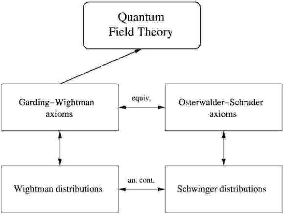
Figure 5: Relations of different axiomatic frameworks for quantum field theory.

The permutation symmetry of the Schwinger functions allows for the construction of a generating functional. In contrast, the Wightman functions are only symmetric for spacelike-separated arguments. Thus, they can not be computed in terms of a generating functional. Another elegant way to define generating functions in Minkowski space is the introduction of Feynman functions which can be defined as “time-ordered” products of field operators:

$$\mathfrak{F}_{n}\left(x_{1},\dots,x_{n}\right)=\langle\Omega|\mathscr{T}\left\{\phi\left[x_{1}\right]\dots\phi\left[x_{n}\right]\right\}|\Omega\rangle\,,$$ (16)

where the time-ordering is defined as the product with factors arranged so that the one with the last time-argument is placed leftmost, the next-latest next to the leftmost etc. [18]. There is also an alternative definition in [28]. It is given by applying a Fourier transform to the Schwinger function and performing an analytic continuation back to Minkowski space afterwards. This is displayed in Fig. 6.

By construction, the Feynman functions are also symmetric for timelike-separated arguments and thus they are symmetric for arbitrary arguments.

Figure 6: Relations between the different kinds of $n$-point functions consisting of vacuum expectation values of products of field operators. The figure has been taken from [28].

Hence, both the Schwinger and the Feynman functions allow for the construction of a generating functional $W_{\mathfrak{S}}\left[J\right]$ and $W_{\mathfrak{F}}\left[J\right]$. Only the Schwinger functions will be considered here — formally the generating functional (sometimes it is also called the vacuum-vacuum functional) is given by

$$W_{\mathfrak{S}}\left[J\right] = \sum_{n=0}^{\infty}\frac{\mbox{i}^{n}}{n!}\int dx_{1}\dots dx_{n}\mathfrak{S}_{n}\left(x_{1},\dots,x_{n}\right)J(x_{1})\dots J(x_{n})$$ (17)

$$= \langle\Omega|\exp\left[\mbox{i}\int d^{4}x\phi[f]J(x)\right]|\Omega\rangle\,,$$

where the functions $J(x_{i})$ are taken from the Schwartz space ${\cal S}\left(\mathbb{R}^{4}\right)$. Using $W_{\mathfrak{S}}[J]$, the Schwinger functions can be recovered by a functional derivative

$$\mathfrak{S}_{n}\left(x_{1},\dots,x_{n}\right)=\frac{\delta^{n}W_{\mathfrak{S}}\left[J\right]}{\delta J_{1}\dots\delta J_{n}}\,.$$ (18)

Knowledge of $W_{\mathfrak{S}}$ is thus equivalent to solving the quantum field theory.

3 The Path Integral

Having now discussed what a quantum field theory is, one needs a recipe of how to construct it. In fact, there exist several prescriptions of how to build a quantum theory if the Lagrangian of the classical field theory to which the quantum theory should reduce is known. The two most commonly used quantization schemes are the canonical quantization scheme (which is described in detail in standard textbooks like [5, 20, 22, 18]) and the path-integral quantization which will be used in this thesis. Both of these schemes break the general covariance of the classical theory discussed in Sec. 2. The quantum theory still stays invariant under global Lorentz transformations (and there even exist generalizations to curved, but fixed spacetimes, see e.g. [29] and references therein), but the quantization prescriptions implicitly assume the existence of a global, canonical basis. However, local Lorentz invariance is only of importance for a quantum theory of gravity, so all to be said in the following can be applied to any quantum theory of strong interactions discussed in Sec. 1.

Construction Principle

Before attempting to define a prescription for a quantum field theory, let us go back to the case of non-relativistic quantum mechanics. The notion of a path integral is closely related to the notion of a random walk. To make this relation obvious, consider the expectation value $\langle E\rangle$ of the evolution operator applied to a single particle in one dimension between two states $|x\rangle,|y\rangle\in{\cal H}$:

$$\langle E\rangle=\langle x|\exp\left[-\mbox{i}\hat{H}t\right]|y\rangle\,.$$ (19)

$\langle E\rangle$ is the probability amplitude for the particle to move from position $x$ to position $y$ in time $t$. If the Hamiltonian corresponds to a free particle,

$$\hat{H}=\frac{\hat{p}^{2}}{2m},$$

then the solution to (19) can be given immediately [24]:

$$\langle E\rangle=\left(\frac{m}{\mbox{i}2\pi t}\right)^{1/2}\exp\left[\mbox{i}\frac{m}{2t}(x-y)^{2}\right]\,.$$ (20)

On the other hand, the probability for a one-dimensional random walk to go from position $x$ to position $y$ in time $t$ is given by [28]:

$$P_{0}(x-y,t)=\left(\frac{1}{4\pi Dt}\right)^{1/2}\exp\left[-\frac{1}{4Dt}(x-y)^{2}\right]\,,$$ (21)

with $D$ being the diffusion constant. The quantum mechanical expectation value is obtained by analytic continuation of Eq. (21) to imaginary time and the identification $D=1/2m$. Thus, the quantum mechanical amplitude may be computed by considering a classical random walk and analytically continuing the result to imaginary time. If one adopts this interpretation, the amplitude can be computed via a path-integral using a conditional Wiener measure, see [28] for a rigorous mathematical treatment.

To extend Eq. (20) also to the case of non-Gaussian Hamiltonians, we decompose the full Hamiltonian $\hat{H}$ into a Gaussian and a non-Gaussian part:

$$\hat{H}=\hat{H}_{0}+\hat{V}(x)\,,$$ (22)

and perform a time-slicing procedure. Consider the evolution operator $\hat{U}(t)=\exp[-\mbox{i}\hat{H}t]$ for small imaginary times $t\rightarrow\mbox{i}\epsilon$. In the leading order, $\hat{U}\left(\mbox{i}\epsilon\right)$ coincides with the operator $\hat{W}\left(\epsilon\right)$ which is defined in the following way:

$$\hat{U}\left(\mbox{i}\epsilon\right)=\hat{W}\left(\epsilon\right)+{\cal O}\left(\epsilon^{3}\right)=\exp\left(\hat{V}\frac{\epsilon}{2}\right)\exp\left(\hat{H}_{0}\epsilon\right)\exp\left(\hat{V}\frac{\epsilon}{2}\right)+{\cal O}\left(\epsilon^{3}\right)\,.$$ (23)

The operator $\hat{W}\left(\epsilon\right)$ is known as the transfer matrix; its matrix elements can be computed to yield:

$$\langle x|\hat{W}\left(\epsilon\right)|y\rangle=\left(\frac{m}{2\pi\epsilon}\right)^{1/2}\exp\left[\frac{m}{2\epsilon}(x-y)^{2}+\frac{\epsilon}{2}\left(V(x)+V(y)\right)\right]\,.$$ (24)

Using the Lie-Trotter formula, one gets:

$$\exp\left[-\left(\hat{H}_{0}+\hat{V}\right)t\right]=\lim_{N\rightarrow\infty}\hat{W}^{N}\left(\epsilon\right)\,.$$ (25)

Inserting $N-1$ times the identity $\mathbf{1}=\int dx_{i}|x_{i}\rangle\langle x_{i}|$ into Eq. (25) finally yields the expression:

$$\langle x|\exp\left[-\hat{H}t\right]|y\rangle = \lim_{N\rightarrow\infty}\left(\frac{m}{2\pi\epsilon}\right)^{N/2}\int dx_{1}\dots dx_{N-1}$$ (26)

$$\quad\times\exp\Biggl{[}-\frac{m}{2\epsilon}\left(\left(x-x_{1}\right)^{2}+\dots+\left(x_{N-1}-y\right)^{2}\right)$$

$$\quad-\epsilon\left(\frac{1}{2}V(x)+V(x_{1})+\dots+V(x_{N-1})+\frac{1}{2}V(y)\right)\Biggr{]}$$

$$= \lim_{N\rightarrow\infty}\left(\frac{m}{2\pi\epsilon}\right)^{N/2}\int dx_{1}\dots dx_{N-1}$$

$$\qquad\qquad\qquad\times\exp\left[-S_{N}\left(x,x_{1},\dots,x_{N-1},y\right)\right]\,.$$

In the continuum limit this equation can now be interpreted as a path integral over a set of random walks with the weight function given in the exponential. If we denote all paths $\omega(\tau)$ with fixed end-points from $\omega(\tau=0)=x_{0}=x$ to $\omega(\tau=t)=x_{N}=y$, then we can write (using the Wiener measure $[\mbox{d}\omega]$):

$$\langle E\rangle = \int[\mbox{d}\omega]\exp\left(-V[\omega]\right)$$ (27)

$$= \lim_{N\rightarrow\infty}\int dx_{1}\dots dx_{N-1}P\left(x_{0},\dots,x_{N}\right)\exp\left(-V\left(x_{0},\dots,x_{N}\right)\right)\,,$$

where

$$P\left(x_{0},\dots,x_{N}\right)=\prod_{i=0}^{N}P_{0}\left(x_{i+1}-x_{i},t_{i+1}-t_{i}\right)\,.$$

Now there is an important difference between the forms of Eqs. (26) and (27): In the latter, the exponential weight which connects neighbor points of the paths is already a part of the measure $[\mbox{d}\omega]$, while in the former the exponential weight is contained in the expression for $S_{N}\left(x_{0},\dots,x_{N}\right)$. What is then the interpretation of this weight factor? From Eq. (2) we know, that any amplitude can be expanded in a power series of $\hbar^{n}$ with the amplitude for the classical process being the leading amplitude. Thus, in the limit $\hbar\rightarrow 0$, only the classical (leading) contribution should contribute to the expression (26). The exponential weight factor should thus be peaked around the classical solution, i.e. the exponential factor will become minimal for the classical trajectory, just like minimizing the action $\mathscr{S}\left[\omega(\tau)\right]$ yields the classical path. Thus, the exponential weight factor in the limit $N\rightarrow\infty$ should coincide with the classical action if one inserts a differentiable trajectory. However, there is an important difference: the classical action $\mathscr{S}\left[\omega(\tau)\right]$ is only defined for differentiable paths, while the exponential factor $\lim_{N\rightarrow\infty}S_{N}(x_{0},\dots,x_{N})$ in (26) is defined for any continuous path (which is a superset of the set of all differential paths). This gives rise to a certain freedom in the choice of $S_{N}(x_{0},\dots,x_{N})$. The actual choice should thus be guided by the desire to simplify the problem at hand. Especially in the case of chiral fermions, a wide class of possible actions has been proposed, see Sec. 4.

Symbolically we can thus introduce a functional $S\left[\omega(\tau)\right]$ which projects any continuous path to a real number and write

$$\langle x|\exp\left[-\hat{H}t\right]|y\rangle=\int{\cal D}x\exp\left[-S\left[x\right]\right]\,,$$ (28)

where the integral measure is given by

$${\cal D}x=\lim_{N\rightarrow\infty}\left(\frac{m}{2\pi\epsilon}\right)^{N/2}dx_{1}\dots dx_{N-1}\,.$$ (29)

The resulting expression Eq. (28) can be analytically continued back to imaginary times using $t\rightarrow\mbox{i}t$ which yields the desired transition amplitude Eq. (20). Such a Wick-rotated form of Eq. (28) is known as the Feynman-Kac formula. Sometimes the derivation is directly carried out in Minkowski space, but the problem is that the integrand is highly oscillatory and not well-defined, for further reading cf. [30].

As already pointed out, the difference between (27) and (28) lies in the interpretation of the measure. One can perform substitutions ${\cal D}x\rightarrow{\cal D}x^{\prime}$ to (29), giving rise to different integral measures. Since the path integral has close resemblance to a system of statistical mechanics (via its affinity to the random walk), we will classify the different classes of paths which can be used in (28) by the means of ensembles. This topic is discussed in detail in Sec. 4. For the time being, we want to interpret (26) as an integral over random paths with a weight given by the entire exponential. This amounts to choosing the measure

$${\cal D}x\propto\lim_{N\rightarrow\infty}dx_{1}\dots dx_{N-1}\,.,$$

Later in Sec. 4 it will be argued that these paths are taken from the random ensemble. In contrast, in the expression (27) using the Wiener measure $[\mbox{d}\omega]$, the paths are taken from the canonical ensemble. This integral measure already contains the kinetic term, but not the potential term. In this way, the problem of assigning a meaning to the derivative from the classical action is circumvented. This procedure is not possible in the case for quantum field theories which will be discussed below since in that case there is no such thing as a Wiener measure.

Computing Observables

As discussed in Sec. 2, one is interested in ground-state expectation values of certain operators, $\langle 0|\hat{A}|0\rangle$. Consider a (countable) Hilbert space ${\cal H}$ with Hamiltonian $\hat{H}$. Let $\{E_{i}\}$, $i\geq 0$, be the eigenvalues and $\{|i\rangle\}$ be the corresponding eigenvectors of $\hat{H}$ in ascending order. Taking the trace of the evolution operator and $\hat{A}$ provides us with

$$\mbox{Tr}\,\left(\hat{A}\exp\left[-\hat{H}\tau\right]\right)=\sum_{i=0}^{\infty}\exp\left[-E_{i}\tau\right]\langle i|\hat{A}|i\rangle\,.$$

In the limit $\tau\rightarrow\infty$ only the term with $E_{0}$ in the exponential survives and we are left with

$$\langle 0|\hat{A}|0\rangle=\lim_{\tau\rightarrow\infty}\frac{1}{Z(\tau)}\mbox{Tr}\,\left(\hat{A}\exp\left[-\hat{H}\tau\right]\right)\,,$$ (30)

with the partition function

$$Z(\tau)=\mbox{Tr}\,\left(\exp\left[-\hat{H}\tau\right]\right)=\sum_{i=0}^{\infty}\exp\left[-E_{i}\tau\right]\,.$$ (31)

For the application to field theory, the operators $\hat{x}(t_{n})$ will require special attention, since they are analogous to the Schwinger functions encountered in Euclidean quantum field theories in Sec. 2). Using $\hat{x}(t)=\exp[\hat{H}t]\hat{x}\exp[-\hat{H}t]$, we consider the $n$-point correlation function $\langle x(\tau_{1})\dots x(\tau_{n})\rangle$, with $\tau_{1}<\dots<\tau_{n}$. It is straightforward [24] to show that

$$\langle 0|\hat{x}(\tau_{1})\dots\hat{x}(\tau_{n})|0\rangle = \lim_{\tau\rightarrow\infty}\frac{1}{Z(\tau)}\mbox{Tr}\,\left(e^{-\hat{H}(\tau/2-\tau_{1})}\hat{x}e^{-\hat{H}(\tau_{1}-\tau_{2})}\dots\hat{x}e^{-\hat{H}(\tau_{n}+\tau/2)}\right)$$ (32)

$$= \lim_{\tau\rightarrow\infty}\frac{1}{Z(\tau)}\int{\cal D}x\,x(\tau_{1})\dots x(\tau_{n})\exp\left[-S\left[x(\tau)\right]\right]\,,$$

where the paths obey periodic boundary conditions,

$$x\left(-\tau/2\right)=x\left(\tau/2\right),$$

and the partition function $Z(\tau)$ can be written as

$$Z(\tau)=\int{\cal D}x\exp\left[-S\left[x(\tau)\right]\right]\,.$$ (33)

Hence, the $n$-point correlation function $\langle x(\tau_{1})\dots x(\tau_{n})\rangle$ is written in (32) as the moment of the measure ${\cal D}x$. There is another possibility to obtain the correlation function from a generating functional $Z_{J}[J(\tau)]$ with $J(\tau)$ being a continuous path by means of the following definition:

$$Z_{J}[J(\tau)] = \lim_{N\rightarrow\infty}\left(\frac{m}{2\pi\epsilon}\right)^{N/2}dx_{1}\dots dx_{N-1}$$ (34)

$$\qquad\times\exp\left[-S(x_{0},\dots,x_{N})+\sum_{i=1}^{n}x_{i}J(\tau_{i})\right]\,.$$

Using

$$\lim_{N\rightarrow\infty}\left(\frac{m}{2\pi\epsilon}\right)^{N/2}\int dx_{1}\dots dx_{N-1}\frac{d}{dJ(\tau_{1})}\dots\frac{d}{dJ(\tau_{n})}$$ (35)

$$\qquad\times\exp\left[-S(x_{0},\dots,x_{N})+\sum_{i=1}^{n}x_{i}J(\tau_{i})\right]$$

$$= \lim_{N\rightarrow\infty}\left(\frac{m}{2\pi\epsilon}\right)^{N/2}\int dx_{1}\dots dx_{N-1}\,x(\tau_{1})\dots x(\tau_{n})$$

$$\qquad\times\exp\left[-S(x_{0},\dots,x_{N})+\sum_{i=1}^{n}x_{i}J(\tau_{i})\right]\,,$$

one recovers Eq. (32). The meaning of the derivatives can be understood by considering again the subset of differentiable paths. The expression then reduces to the functional derivative. Thus, $Z_{J}[J(\tau)]$ can be considered to be the generating functional for the $n$-point correlation functions and we can write symbolically:

$$\langle x(\tau_{1})\dots x(\tau_{n})\rangle=\lim_{\tau\rightarrow\infty}\frac{\delta^{n}Z_{J}[J(\tau)]}{\delta J(\tau_{1})\dots\delta J(\tau_{2})}\,.$$ (36)

Here the notation of the conventional functional derivative has been employed, but with a meaning corresponding to Eq. (35. This expression is similar to the generating functional of the Schwinger functions (18), implying that generalizing $Z_{J}[J(\tau)]$ to the case of Euclidean fields is the key to find a quantization prescription for quantum field theories.

Euclidean Field Theory

The generalization of Eq. (36) to the case of Euclidean fields is very difficult, however. As a starting point one can expect that the expectation values for the Schwinger function in (15) can also be written using a path integral just like the $n$-point functions in (32). They would then be moments of some suitably defined measure

$$[\mbox{d}\phi]=\mathscr{N}\exp\left[-S\left[\phi\right]\right]{\cal D}\phi\,.$$ (37)

The Schwinger functions $\mathfrak{S}_{n}(x_{1},\dots,x_{n})$ can hence be written

$$\mathfrak{S}_{n}(x_{1},\dots,x_{n})=\frac{1}{W_{\mathfrak{S}}[0]}\int[\mbox{d}\phi]\phi(x_{1})\dots\phi(x_{n})\,,$$ (38)

where the generating functional $W_{\mathfrak{S}}[0]$ is the field theory analogue of Eq. (33). It can symbolically be written as

$$W_{\mathfrak{S}}[0]=\int[\mbox{d}\phi]\equiv Z\,.$$ (39)

The functional $S[\phi]$ appearing in Eq. (37) is again a suitable generalization of the Euclidean action to a superset of continuous, but non-differentiable fields. The vacuum expectation value $\langle\hat{A}\rangle=\langle\Omega|\hat{A}|\Omega\rangle$ of a general operator, $\hat{A}\left[\phi(x)\right]$, is then defined by the path integral

$$\langle\hat{A}\rangle=Z^{-1}\int[\mbox{d}\phi]\,\hat{A}\left[\phi\right]\,,$$ (40)

where the partition function $Z$ is given by (39). However, this definition encounters severe difficulties because of the fact that the $\phi[f]$ are not pointwise-defined objects.

By inverting the logic which led to the path-integral formula Eq. (27), one can define a prescription to formulate a quantum field theory starting from a classical action $\mathscr{S}$. This procedure which gives meaning to Eq. (37) is called renormalization theory and consists of the following steps [21]:

1. Regularize the theory by imposing an ultraviolet cutoff $\Lambda=a^{-1}$ (where $a$ is a distance short compared to the intrinsic scales of the theory) so that (37) is a well-defined measure. This can e.g. be done by discretizing the Euclidean space $\mathbb{R}^{4}$ to describe the system using a (finite) lattice in $\mathbb{Z}^{4}_{\Omega}$ such that all $\{x_{i}\}\in\mathbb{Z}^{4}_{\Omega}$. Find a functional $S_{\{g_{i}\}}[\phi(x)]$ with parameters $\{g_{i}\}$ on the lattice which reduces to the classical action $\mathscr{S}[\phi(x)]$ for differentiable continuum fields. This prescription is not unique. In any case, however, either Euclidean invariance or Osterwalder-Schrader positivity or both are broken. Let $\langle\phi(x_{1})\dots\phi(x_{n})\rangle_{\{g_{i}\}}$ be the $n$-point functions of the discrete theory.

2. Perform the infinite volume limit $\Omega\rightarrow\infty$ for the system with $\{g_{i}\}$ held fixed. This limit must exist and be unique.

3. Allow the parameters $\{g_{i}\}$ of $S_{\{g_{i}\}}\left[\phi\right]$ to be functions of $\Lambda$: $\{g_{i}\}\mapsto\{g_{i}\left(\Lambda\right)\}$. The parameters occurring in (37) are then called the bare parameters.

4. Perform the continuum limit $\Lambda=a^{-1}\rightarrow\infty$. A continuum quantum field theory is obtained from the sequence of lattice theories by rescaling the lengths by a factor $\Lambda$ and rescaling the fields by a factor $Z(\Lambda)$:

   $$\mathfrak{S}_{n}(x_{1},\dots,x_{n})=\lim_{\Lambda\rightarrow\infty}Z(\Lambda)^{n}\langle\phi(x_{1})\dots\phi(x_{n})\rangle_{\{g_{i}(\Lambda)\}}\,.$$ (41)

   For each choice $\{g_{i}\left(\Lambda\right)\}$ check the convergence properties of $\mathfrak{S}_{n}$ and if they satisfy the Osterwalder-Schrader axioms.

5. Consider all possible choices of $\{g_{i}(a^{-1})\}$ and $Z(a^{-1})$; classify all limiting theories $\mathfrak{S}_{n}(x_{1},\dots,x_{n})$ and study their properties.

This procedure may give rise to continuum theories which can be categorized as follows:

No limit:

For at least one $n$, the limit (41) does not exist.

Unimportant limit:

All resulting $\{\mathfrak{S}_{n}\}$ exist, but are devoid of information (like $\mathfrak{S}_{n}=0\ \forall n$ etc.)

Gaussian limit:

The limiting theory $\{\mathfrak{S}_{n}\}$ is Gaussian, i.e. a generalized free field. This situation is commonly referred to as triviality.

Non-Gaussian limit:

The limiting theory is non-Gaussian giving rise to a nontrivial theory. This may, however, still imply that the scattering matrix is the identity.

For a non-trivial limit to exist, the lattice theories should have correlation lengths $\xi(\Lambda)\simeq\Lambda^{-1}\xi\{g_{i}(\Lambda)\}$ as $\Lambda\rightarrow\infty$ (otherwise the physical lengths would get rescaled to $0$). Thus, the parameters $\{g_{i}(a^{-1})\}$ should approach or sit on the critical surface and the theory must undergo a phase transition of second order where the correlation lengths diverge. This is expected to be the case for most interesting quantum field theories whose critical behavior can be handled using the renormalization group of Wilson, see [31] for the historical paper and [24, 32] for standard textbooks. There is also a second very interesting case where $\xi\{g_{i}(\Lambda)\}=\infty$ for all $\Lambda$, i.e. the parameters $\{g_{i}\}$ already sit on the critical surface for finite lattice spacings. This is e.g. the case in non-compact U$(1)$ pure gauge theories. For compact U$(1)$ the situation is less clear so far, consult for a description of simulation results the work of Arnold [33] and references therein..

Despite the huge phenomenological successes of quantum field theories in practice, a rigorous proof that the resulting theory exists in the sense defined above, has been stated so far only for a few special cases. In four dimensions, so far only free fields have been proven with mathematical rigor to give rise to a relativistic quantum field theory.

Evaluation of Path Integrals

Having now a definition for the path integral, we also need a way to evaluate it. In principle there are two different ways to compute expressions of the form (28) and (40):

• Consider a series of weight factors $\left\{\exp\left[-S_{i}\right]\right\}$, $i=1,\dots,N$, which converges to the desired weight factor $\lim_{i\rightarrow\infty}\exp\left[-S_{i}\right]=\exp\left[-S\right]$. The path integrals (28) should be computable for each $\exp\left[-S_{i}\right]$.

• Compute an approximation to (28) for finite $N$ in the measure (29). The resulting approximation will depend on $N$. Then perform the limit $N\rightarrow\infty$.

As has already been mentioned, taking the limit in (41) is only possible in some simple models, or in the case that the resulting integrals have Gaussian shape. One way to also extend the applicability to non-Gaussian models is thus to approximate the “true” function $W_{\mathfrak{S}}$ by integrable Gaussian models which reduce to the $W_{\mathfrak{S}}$ in some suitable limit.

The most popular form to do this is to expand the exponential into a Gaussian part and a small, non-Gaussian part:

$$\exp\left[-S[\phi]\right]=\exp\left[-S_{\mbox{\tiny Gaussian}}\right]\sum_{n=0}^{\infty}\frac{1}{n!}\frac{\delta^{n}\left(\exp\left[-(S-S_{\mbox{\tiny Gaussian}})[\phi]\right]\right)}{\delta\phi^{n}}\,.$$ (42)

The idea is then to form the path-integral of the r.h.s. of Eq. (42) and take the result to be the sum of all contributions. The problem behind the series obtained this way is that in several cases the sum fails to converge. This is the case of the common four-dimensional models, as has first been noted by Dyson in [34].

As an example consider the “field theory” at a single site with “partition function” [35]

$$Z=\frac{1}{\sqrt{2\pi}}\int_{-\infty}^{\infty}d\phi\;\exp\left(-\phi^{2}/2+g\phi^{4}\right)\,.$$ (43)

The function $Z=Z(g)$ contains an essential singularity at the origin. Performing the perturbative expansion (42) yields

$$Z=\sum_{k=0}^{\infty}g^{k}Z_{k},\quad Z_{k}=\frac{(-1)^{k}}{k!}\sqrt{\frac{2}{\pi}}\int_{0}^{\infty}d\phi\;\exp\left(-\phi^{2}/2+4k\ln\phi\right)\,,$$

which has a convergence radius of $g=0$. Performing a semi-classical expansion around the saddle point $\phi_{c}=2\sqrt{k}$ and integrating over the quadratic deviations yields

$$Z_{k}\approx\frac{(-16)^{k}}{\sqrt{\pi}}\exp\left((k-1/2)\ln k-k\right)\,.$$

Obviously the $Z_{k}$ are divergent (and the divergence is in fact logarithmic), but the power series is at least asymptotic in the complex $g$ plane cut along the negative real axis since

$$\left|Z(g)-\sum_{k=0}^{\infty}g^{k}Z_{k}\right| < \frac{4^{n+1}\Gamma(2n+3/2)}{\sqrt{\pi}(n+1)!}\frac{|g|^{n+1}}{(\cos(1/2\mbox{Arg}\,g))^{2n+3/2}}\,.$$

This means that for fixed $n$ the right hand side can be made arbitrarily small by choosing $g$ small enough. It may even be possible to recover the full partition function $Z$ from the series expansion $\{Z_{k}\}$ using resummation. For recent reviews of the application of resummation techniques consult [36, 37].

Despite these conceptional difficulties, perturbation theory turns out to be the most effective approach to treat many problems in quantum field theory provided the expansion parameter is sufficiently small. However, in several situations of interest, the latter condition is not fulfilled and the perturbative expansion is not even asymptotic, or the expansion parameter is too large, causing it to diverge already in the lowest orders. In these situations, one has to resort to different ways to approximate the Schwinger functions. One possibility is a numerical simulation of Euclidean QFT on the finite, discrete lattice $\mathbb{Z}^{4}_{\Omega}$. It has some very intriguing advantages: it does not resort to any assumptions of the dynamics of the model one is examining other than the information underlying the regularized action and it is directly based on the definition of the quantities under consideration. In essence, any operator $\hat{A}\left[\phi(x)\right]$ corresponding to a physical observable can be written via (40) as the corresponding moment of a measure $[\mbox{d}\phi]$ on the underlying space. The ensemble of field configurations $\phi(x)$ is distributed according to the partition function (39). Consequently, the latter is the quantity which one tries to access in numerical simulations.

However, this approach has the shortcoming that the actual continuum limit can never be performed and at best one has to resort to extrapolation techniques giving rise to further uncertainties. Since the actual shape of the Schwinger functions is not recovered, an analytic continuation to Minkowski-space is not possible either and objects like distribution amplitudes are not directly accessible. Nonetheless it is possible to compute integrals over these functions and their moments, which help to shed light on their behavior. This approach has been used in e.g. [38, 39, 40, 41, 42, 43] to extract information about form factors and structure functions from lattice simulations.

One important question is if the theory is renormalizable if one uses a perturbative expansion. There are models which are renormalizable non-perturbatively, but are non-renormalizable when employing a perturbative expansion. This is the case for the Gross-Neveau model at large $N$ in three dimensions [21].

However, due to the great importance of perturbative methods, the models which are perturbatively renormalizable are considered in most practical applications. This means that one has to choose Lagrangians with mass dimension $d(\mathscr{L})\leq 4$ [35], where the mass dimension for the scalars $\phi$, Dirac spinors $\psi$ and vector fields $A^{\mu}$ and their derivatives are given by:

$$d(\phi)=1\,,\qquad d(\partial^{n}\phi)=1+n\,,$$

$$d(\psi)=3/2\,,\qquad d(\partial^{n}\psi)=3/2+n\,,$$

$$d(A^{\mu})=1\,,\qquad d(\partial^{n}A^{\mu})=1+n\,.$$ (44)

The mass dimension of a composite term in the Lagrangian is given by adding the mass dimensions of its factors. A dimension-four term then corresponds to a renormalizable interaction, less than four is super-renormalizable and greater than four is non-renormalizable.

4 Ensembles

Following its definition, Eq. (40), the quantum mechanical vacuum expectation value $\langle\hat{A}\rangle$ of some functional $\hat{A}\left[\phi\right]$ of the fundamental fields in the theory, $\phi(x)$, can be written as the moment of the measure (37). As discussed in Sec. 3, the analytic treatment of equation (40) is only possible in case the path integral has the shape of a Gaussian or in some toy models. If one does not want to recourse to expansion techniques or simplifying assumption at this stage, the only alternative method known today is the numerical treatment of (40). However, a straightforward integration does not appear to be feasible, since the dimensionality of the integral in simulations as they are run today is easily exceeding $10^{6}$ [44]. The only alternative is therefore a Monte-Carlo integration. To define possible techniques for treating this problem, the concept of ensembles of configurations has turned out to be extremely useful [24]:

Ensembles:

An ensemble $\left(\{{\phi}\},\rho\{{\phi}\},[\mbox{d}\phi]\right)$ consists of an infinite number of field configurations $\{{\phi}\}$ with a density $\rho\{{\phi}\}$ defined on the measure $[\mbox{d}\phi]$.

A simple example is the micro-canonical ensemble, which is defined by

$$\rho\{{\phi}\}_{\mbox{\tiny$\mu$-can}}\propto\delta\left(S\left[\phi\right]-C\right)\,,$$ (45)

with a constant $C\in\mathbb{R}^{1}$. Thus, this ensemble only consists of configurations with a fixed action. Obviously, this ensemble cannot be used for the evaluation of (40), since the majority of configurations appearing in the path-integral are not members of $\{{\phi}\}_{\mbox{\tiny$\mu$-can}}$. To take account of the need to include any possible configuration in the ensemble, we also have to introduce the notion of ergodicity:

Ergodicity:

An ensemble $\left(\{{\phi}\},\rho\{{\phi}\},[\mbox{d}\phi]\right)$ is called ergodic if

$$\rho\{{\phi}\}>0\quad\forall\phi\in\mathbb{E}^{4}\,.$$

An example of an ergodic ensemble is given by the random ensemble, where each possible field configuration enters with equal probability:

$$\rho\{{\phi}\}_{\mbox{\tiny rand}}\propto 1\,.$$ (46)

With the measure $[\mbox{d}\phi]_{\mbox{\tiny rand}}$ from the random ensemble, the expression (40) becomes

$$\langle A\rangle=Z^{-1}\int[\mbox{d}\phi]_{\mbox{\tiny rand}}\;e^{-S[\phi]}A\left[\phi\right]\,,\qquad Z=\int[\mbox{d}\phi]_{\mbox{\tiny rand}}\;e^{-S[\phi]}\,.$$ (47)

Switching to different ensembles in path integrals consists of a re-parameterization of the measure. It is therefore equivalent to the substitution rule in ordinary integrals.

Another example of an ergodic ensemble is given by the canonical ensemble (also known as the “equilibrium ensemble”) which is defined by

$$\rho\{{\phi}\}_{\mbox{\tiny can}}\propto e^{-S\left[\phi\right]}\,.$$ (48)

The measure in (37) is corresponding to the canonical ensemble and therefore underlying the path integral definition in Eq. (40). Due to this simple form of the operator expectation value, the canonical ensemble (48) plays a huge role in numerical simulations of quantum field theories.

Finally an important generalization of the canonical ensemble is given by the multi-canonical ensemble. Suppose the underlying action in Eq. (48) is replaced by an action $S\left[\phi\right]\rightarrow S^{{}^{\prime}}\left[\phi\right]=S\left[\phi\right]+\gamma\tilde{S}\left[\phi\right]$, with some parameter $\gamma$. The ensemble $\{\phi\}^{\gamma}_{\mbox{\tiny multi-can}}$ with density

$$\rho\{{\phi}\}^{\gamma}_{\mbox{\tiny multi-can}}\propto e^{-S^{{}^{\prime}}\left[\phi\right]}$$ (49)

leads to the following shape of (40):

$$\langle\hat{A}\rangle=Z_{\gamma}^{-1}\int[\mbox{d}\phi]^{\gamma}_{\mbox{\tiny multi-can}}\;e^{\gamma\tilde{S}\left[\phi\right]}A\left[\phi\right]\,,\qquad Z_{\gamma}=\int[\mbox{d}\phi]^{\gamma}_{\mbox{\tiny multi-can}}\;e^{\gamma\tilde{S}\left[\phi\right]}\,.$$ (50)

The reason why (49) is useful is that it is often possible to find an action $S^{\prime}\left[\phi\right]$ which is numerically simpler to handle and simulate than the original action $S\left[\phi\right]$ and with the ensembles (48) and (49) being close enough to each other such that the “reweighting correction” in (50) is small. A situation where this is the case is given in this thesis in the framework of the TSMB algorithm to be discussed in Sec. 3.

The ensemble is given by an infinite set of field configurations $\{{\phi}\}$. The introduction of ensembles thus apparently made the problem of integrating a complicated multi-dimensional system even worse instead of simplifying it. However, the re-formulation of the problem allows for a solution by a different integration technique, the Monte-Carlo integration [24, 32, 45]. This numerical method is going to be discussed in Sec. 1.

4 Gauge Theories

The guiding principle of the construction of quantum field theories in Sec. 2 was the idea of locality. For a start, consider the $N$-component ($N\geq 2$) Yang-Mills theory described by the Lagrangian:

$$\mathscr{L}\left(\bar{\Psi}_{N},\Psi_{N}\right)=\bar{\Psi}_{N}\left(\mbox{i}/\!\!\!\partial-m\right)\Psi_{N}\,,$$ (51)

which is invariant under global transformations $U\in\mbox{SU}(N)$:

$$U:\left\{\begin{array}[]{l}\Psi_{N}\mapsto\Psi_{N}^{\prime}=U\,\Psi_{N},\\ \bar{\Psi}_{N}\mapsto\bar{\Psi}_{N}^{\prime}=\bar{\Psi}_{N}\,U^{\dagger}\,.\end{array}\right.$$ (52)

However, a global transformation on the fields living in $\mathbb{R}^{4}$ is not consistent with the idea of locality. Rather we want a theory which is invariant under local gauge transformations $U(x)\in\mbox{SU}(N)$:

$$U(x):\left\{\begin{array}[]{l}\Psi_{N}\mapsto\Psi_{N}^{\prime}=U(x)\,\Psi_{N},\\ \bar{\Psi}_{N}\mapsto\bar{\Psi}_{N}^{\prime}=\bar{\Psi}_{N}\,U^{\dagger}(x)\,.\end{array}\right.$$ (53)

A theory invariant under these transformations is called a gauge theory. It is possible to add to Eq. (51) a term containing a new set of fields $A^{\mu}_{a}(x)$ such that it stays invariant under the transformation (53). The simplest way to do this is to choose

$$\mathscr{L}(\Psi_{N},\bar{\Psi}_{N},A^{\mu}_{a})=\bar{\Psi}_{N}\left(\mbox{i}\ /\!\!\!\!D-m\right)\Psi_{N}\,,$$ (54)

where the covariant derivative $/\!\!\!\!D$ is given by

$$/\!\!\!\!D=\gamma_{\mu}\left(\partial^{\mu}+\mbox{i}gA^{\mu}_{a}\right)\,,$$ (55)

and the transformation of $A^{\mu}_{a}(x)$ must be given by

$$U(x):A^{\mu}_{a}(x)\mapsto{A^{\mu}_{a}}^{\prime}(x)=U^{\dagger}(x)\left(\partial^{\mu}+A^{\mu}_{a}(x)\right)U(x)\,,$$ (56)

meaning that the $A^{\mu}_{a}$ lie in the adjoint representation of SU$(N)$ and that $1\leq a\leq\mbox{dim}\left(\mbox{SU}(N)\right)$. Thus, the resulting theory will now contain the fields $\bar{\Psi}_{N}$, $\Psi_{N}$, and $A^{\mu}_{a}(x)$. The new fields $A^{\mu}_{a}(x)$ are termed gauge fields and their coupling to the fields $\bar{\Psi}_{N}$, $\Psi_{N}$ is given by the dimensionless coupling strength $g$.

By postulating the fields to be invariant under the transformations (53) and (56) and requiring that the Lagrangian only contains perturbatively renormalizable terms (see Sec. 3), one is finally led to the general form

$$\mathscr{L}(\bar{\Psi}_{N},\Psi_{N},A^{\mu})=-\frac{1}{4}\sum_{a=1}^{N^{2}-1}F_{\mu\nu}^{a}F^{\mu\nu a}+\bar{\Psi}_{N}\left(\mbox{i}\ /\!\!\!\!D-m\right)\Psi_{N}\,,$$ (57)

with the field strength

$$F_{\mu\nu}^{a}=\partial_{\mu}A_{\nu}^{a}-\partial_{\nu}A_{\mu}^{a}+g\sum_{b,c=1}^{N^{2}-1}f_{abc}A_{\mu}^{b}A_{\nu}^{c}\,.$$ (58)

There is an important difference between the pure gauge part in the SU$(N)$ Lagrangian (57) and the single gauge field Lagrangian (9) corresponding to an Abelian gauge group: The former contains interactions between different components of the gauge field $A^{\mu}_{a}$, while the latter describes a true free field. Thus, the $N$-component vector theory contains interactions even in the case of a purely gauge theory without coupling to a matter field. It is argued below, that this phenomenon leads to the dynamical generation of a mass scale in the case of the quantized theory. This phenomenon is also known as dimensional transmutation.

Since the group SU$(N)$ is non-Abelian — their elements don’t commute — Eq. (57) is referred to as a non-Abelian gauge theory. For alternative ways to define a gauge theory cf. [46, 24] and references therein.

In addition to the SU$(N)$ symmetry, the Lagrangian (57) is also invariant under axial rotations of the fermion fields, provided, the Dirac part is massless ($m=0$):

$$\Psi\mapsto\Psi^{\prime} = \exp\left[\gamma_{5}\alpha\right]\Psi\,,$$

$$\bar{\Psi}\mapsto\bar{\Psi}^{\prime} = \bar{\Psi}\exp\left[-\gamma_{5}\alpha\right]\,.$$ (59)

The question arises, whether this symmetry exists also on the quantum level, or if it is broken by an anomaly. As has been realized by Adler [47] and Bell and Jackiw [48], for an Abelian gauge theory this is indeed the case. The anomaly responsible for breaking the axial current corresponding to the symmetry (4) is known as the Abelian anomaly or ABJ-anomaly. It is present once the theory contains fermions and is independent of the fermion masses. This result has also been derived non-perturbatively by Fujikawa [49]. An extension to non-Abelian theories has been given in [50]. For a textbook containing a rigorous mathematical treatment consult [51].

5 Quantum Chromodynamics

Now the ground has been prepared to formulate quantum chromodynamics (QCD) as the theory underlying the strong interaction. It is a Yang-Mills gauge theory (see Sec. 4) symmetric under the SU$(3)$ group (as discussed in Sec. 1), where the latter symmetry group refers to the color degree of freedom of the quarks. It contains six flavors of quarks with masses $\{m_{k}\}$, with each flavor of quarks transforming as the fundamental triplet representation of the color group. The accompanying vector bosons, the “gluons” transform according to the adjoint representation. Furthermore we require the theory to be perturbatively renormalizable. Thence, the resulting Lagrangian $\mathscr{L}_{\mbox{\tiny QCD}}$ in Minkowski-space is given by (the number of colors is denoted by $N_{c}=3$)

$$\mathscr{L}_{\mbox{\tiny QCD}}=-\frac{1}{4}\sum_{a=1}^{8}G_{\mu\nu}^{a}G^{\mu\nu a}+\sum_{k=1}^{6}\sum_{\alpha=1}^{N_{c}}\bar{\Psi}_{k\alpha}\left(\mbox{i}\ /\!\!\!\!D-m_{k}\right)\Psi_{k\alpha}\,.$$ (60)

It is also possible (without violating perturbative renormalizability) to add a term of the form

$$\mathscr{L}_{\theta}\propto\frac{\theta g^{2}}{64\pi^{2}}\sum_{a=1}^{8}\varepsilon_{\alpha\beta\mu\nu}G^{\alpha\beta a}G^{\mu\nu a}$$

to (60). This term is known as the “$\theta$-term” and would be a source of $CP$ violation [11]. The experimental limit for $\theta$ is ${\cal O}(10^{-9})$. Thus, this term will not be considered in this thesis.

Several important properties of QCD can be learned by considering the symmetries of (60) [35]. For $N_{f}$ massless quark flavors, $\mathscr{L}_{\mbox{\tiny QCD}}$ is invariant under several global symmetry transformations. In particular, one can decompose the Dirac spinors into left- and right-handed quark fields and perform independent rotations on the resulting Weyl spinors. This yields a global $\mbox{SU}(N_{f})_{L}\otimes\mbox{SU}(N_{f})_{R}$ symmetry (this symmetry is also known as chiral). Furthermore one can make independent global vector and axial rotations on the full Dirac spinors resulting in a global $\mbox{U}(1)_{V}\otimes\mbox{U}(1)_{A}$ symmetry. When looking at the masses of the different quark flavors, one can indeed consider the masses of the $u$- and $d$- quark flavors to be almost zero compared to the typical scales of hadronic resonances. To a lesser extent this is also valid for the $s$-quark flavor. Thus, QCD contains three almost massless fermion flavors and should consequently have a global $\mbox{SU}(3)_{L}\otimes\mbox{SU}(3)_{R}\otimes\mbox{U}(1)_{V}\otimes\mbox{U}(1)_{A}$ symmetry.

According to the Noether theorem, there should be conserved charges corresponding to each symmetry of the Lagrangian. The U$(1)_{V}$-symmetry is indeed associated with a conserved quantum number, namely the baryon number which is conserved exactly by the strong interaction. The current corresponding to the axial U$(1)_{A}$-symmetry is, however, explicitly broken by the ABJ anomaly (cf. Sec. 4) if the theory is quantized. Nonetheless, one can find a modified, conserved current albeit it will be gauge-dependent and thus not represent a physical current.

From the remaining chiral symmetry, one half is indeed present in the hadron spectrum, namely as the flavor SU$(3)_{F}$ symmetry discussed in Sec. 1. This half corresponds to a vector symmetry transformation of the Dirac spinors. The other half, however, which corresponds to an axial vector transformation would result in a parity degeneracy of the particles which is clearly not observed. To be specific, there are no parity degeneracies present in the hadron spectrum at all. Thus, the quantization of QCD must break this symmetry. Since there is no anomaly which could attribute for this symmetry breaking, it must be broken in a spontaneous manner, i.e. the ground state of the theory will not be invariant. Due to the Goldstone theorem [35], consequently there exist massless particles corresponding to the pseudoscalar mesons whose masses are much smaller than those of the other hadrons. The fact that they are not zero can be attributed to the explicit breaking of chiral symmetry due to the small masses of the light quarks. Within the framework of Chiral Perturbation Theory ($\chi$PT) (see Sec. 3), it can indeed be shown that for small quark masses, the effect can be treated perturbatively.

But there does not seem to exist any Goldstone boson corresponding to the breaking of the axial U$(1)_{A}$ charge. The only particle with the correct symmetries is the $\eta^{\prime}$-meson whose mass is far too large (see Tab. 1). The solution of this problem is related to the topology of the gauge field. Topological transitions can produce the $\eta^{\prime}$-mass via the axial anomaly. A possible explanation is that instanton transitions (see below) are responsible for these topological charge fluctuations.

1 Running Coupling and Energy Scales

The quantum theory build upon (60) is characterized by a running coupling (for details see e.g. [35]). Performing a leading order perturbative analysis and renormalizing the theory, the behavior of the running coupling “constant” is found to be

$$\alpha_{S}(Q^{2})=\frac{4\pi}{\beta_{0}}\frac{1}{\ln\left(Q^{2}/\Lambda_{\mbox{\tiny QCD}}^{2}\right)}\,,$$ (61)

with $\beta_{0}=11-2/3N_{f}$, where $N_{f}$ is the number of active flavors [11]. This defines the coupling at an energy scale $Q^{2}$. There are two important lessons to be learned from (61):

• The coupling $\alpha_{S}(Q^{2})$ decreases for increasing values of $Q^{2}$. The interaction vanishes for $Q^{2}\rightarrow\infty$ and the particles becomes free in this limit. This property is referred to as asymptotic freedom.

• The coupling becomes infinite for a certain finite value of $Q^{2}$, $\Lambda^{2}_{\mbox{\tiny QCD}}$. This happens also in case of an Abelian gauge theory (where the underlying group is U$(1)$) and shows an intrinsic inconsistency under which (61) has been derived: The assumption that $\alpha(Q^{2})$ is small becomes invalid for increasing $\alpha_{S}(Q^{2})$ at some point and the series starts to diverge already at the first order beyond tree level. This singularity is called the Landau pole and is considered to be an unphysical remnant only present due to the fact that perturbation theory cannot be applied for too large expansion parameters. The appearance of the Landau pole thus sets a limit to the applicability of perturbative calculations. On the other hand one can expect the calculation to be valid at energies far larger than $\Lambda_{\mbox{\tiny QCD}}$.

It is usually assumed that, when “solving” full QCD by the methods sketched in Sec. 3, one also obtains the whole low-energy phenomenology with minimal input. There is no reason why the failure of a single method, namely the perturbative expansion around the free field, should imply that QCD is not valid at low energy scales. However, a concise solution of interacting quantum field theories is not in sight, so one has to stick with a number of models parameterizing the low-energy behavior. One of these parameterizations is $\chi$PT [52]. Besides the latter, there are also different effective theories which parameterize the behavior of the strong interaction at low energies: models like the Nambu-Jona-Lasignio model [53], the skyrmion model [54], or models based on instantons (see below) are different attempts to describe the properties of low energy strong interactions. The hadrons built up from one of the three heavy quarks can be described using Heavy-Quark Effective Theory (HQET), see [55, 56] for introductions.

However, all these theories are only able to predict the low-energy properties of the strong interaction; they do not incorporate an adequate mechanism for the description of the parton content of hadrons. For the high energy regime, the perturbative treatment of QCD has to be used, which describes the interaction using the color group with the gluons being the mediators of the strong force. However, if the strong interaction is described using the flavor group as an interaction between the baryons (the octet multiplet in the flavor SU$(3)$ group), then the mediating particles are the pseudoscalar mesons.

One particularly important concept in the development of QCD is the hypothesis of confinement. The common understanding of confinement is that in a world without sea quarks, the static potential of two quarks would be linear growing without limit. This leads to bound quarks not being separable and thus free quarks being unobservable. One consequence of this picture of confinement could be that the classical limit, Eq. (2), may not exist. Thus, the consequences of confinement could be wide-reaching. The best tools which have so far been used to address this particular issue are lattice simulations. For a recent discussion of lattice simulations regarding confinement, see [57] and references therein.

There is another very important property of QCD shared with other non-Abelian gauge theories: Consider (57) without fermions. Then it can be shown [58] that there exist gauge field configurations which vanish at spatial infinity, but fall into different topological classes. They may be characterized by the winding number $n(U)$, which is given by the Chern-Simons three form on the gauge fields [59, 51]. The transition between the different topological sectors may be performed using the instanton solutions. These are solutions of the classical equations of motion and they may also contribute significantly in the quantized theory. For recent overviews consult [60, 61, 62]. The importance of instantons for hadron physics has also been demonstrated on the lattice in [63, 64]. Recently, a method to examine a prediction of the instanton model with lattice simulations has been proposed in [65]. This method has been applied in [66], confirming the predictions of the instanton model. Indications for this picture have also been found in an earlier publication [67] and in later works [68, 69].

One particularly important point is that the quantum field theory built upon (57) puts a lower limit to the magnitude of the instanton actions resulting in a certain mass scale of the theory. Thus, a mass-scale is generated although the classical theory is scale-free (and has no free parameters except for the coupling $g$ which can be rescaled to any value). As has already been mentioned in Sec. 4, this phenomenon is known as dimensional transmutation. A different widely discussed manifestation of dimensional transmutation is the existence of glue-balls (see e.g. [70] for a recent overview).

2 Factorizable Processes

Several observables in QCD (like structure functions and form factors etc., see e.g. [71, 72] and for a more recent review [73] and references therein) depend on input from both regimes. For several interesting processes involving these observables, a method known as factorization is applicable. The formal framework of factorization is the operator-product expansion, whenever it applies. Consider two local operators $\hat{A}(x)$, $\hat{B}(y)$. The Wilson expansion of the time ordered product of the composite operator for short distances $(x-y)\rightarrow 0$ can then be performed as [74]

$$\mathscr{T}\left\{\hat{A}(x)\hat{B}(y)\right\}=\sum_{i}C_{i}(x-y)\hat{N}_{i}(x)\,.$$ (62)

This relation is only established perturbatively, however. The singularities of the composite operator $T\left\{\hat{A}(x)\hat{B}(y)\right\}$ are then contained in the $\{C_{i}\}$ which are $C$-numbers. They are called Wilson coefficients and contain the high-energy physics. Consequently, they can be computed perturbatively. The operators $\{\hat{N}_{i}\}$ are local operators containing information about the low-energy regime and hence are usually not accessible by perturbative methods. The individual terms in the sum (62) can be arranged in such an order that the single terms behave as a power series in $Q^{-2N}$, where $N$ characterizes the order of the associated term. This is done by ascribing a certain “twist” to each term. The first term (which vanishes slowest) is called the “leading twist contribution” and the higher terms are consequently “higher twist contributions”. The series then takes a form reminiscent of the perturbative expansion, Eq. (42).

In the form of (62), the high energy regime and the low energy part can be treated separately, and the object under consideration factorizes in the two separate contributions. The major ingredient to a factorization scheme is the factorization scale, i.e. the scale describing which contributions belong to the low-energy regime and thus, to the operators $\hat{N}_{i}(x)$, and which contributions belong to the high energy part, i.e. the functions $C_{i}(x-y)$. This leaves a certain freedom in the application of the factorization approach. This freedom should be exploited to keep higher-order corrections in the perturbative series as small as possible, shifting the majority of contributions into the leading order.

Naturally the question arises to what extent it is possible to ascribe any meaning to a series like (62) if it involves a running coupling (61) which is singular at some point in the physical parameter space. This question has been addressed in e.g. [75]. From a pragmatic point of view one can adopt the series despite the conceptional problems. However, one has to circumvent the Landau singularity; to achieve this, a number of proposals have been made: one is to apply a “freezing” prescription, i.e. simply hold the coupling constant fixed below a certain point [76]. Another consists of introducing an effective gluon mass [77]. A different approach relies on the application of an analytization procedure (first applied to QED by Lehmann and then Bogoliubov, see [78, 79, 80] and references therein), which was originally invented to extent (61) also to the regime where $Q^{2}$ is a timelike momentum transfer [81, 82]. Later a framework of analytic perturbation theory has been founded on this bases by Shirkov and Solovtsov in [83, 84, 85, 86]. In essence, the Landau singularity in Eq. (61) can be compensated in a minimal way by adding a unique power-term replacing the running coupling by

$$\alpha_{S}(Q^{2})=\frac{4\pi}{\beta_{0}}\left(\frac{1}{\ln\left(Q^{2}/\Lambda_{\mbox{\tiny QCD}}^{2}\right)}+\frac{\Lambda_{\mbox{\tiny QCD}}^{2}}{\Lambda_{\mbox{\tiny QCD}}^{2}-Q^{2}}\right)\,.$$ (63)

In contrast to the conventional expansion, the contribution of higher terms appears to be suppressed (cf. [84]). This observation together with a renormalization and factorization scheme optimized for putting most higher order contributions into the leading order should allow for a consistent and efficient description of factorizable processes. Indeed, it has been found that this program works for the cases of the electromagnetic form factor of the pion and the $\pi\rightarrow\gamma^{*}\gamma$ transition form factor [87, 88, 89] and yields an excellent agreement with the experimental data while providing a consistent framework for the computation of hadronic observables.

3 Lattice QCD

The approach to perform a numerical simulation on a finite lattice yielding an approximation to the Schwinger functions $\mathfrak{S}_{n}$ in discrete Euclidean space $\mathbb{Z}^{4}_{\Omega}$ is referred to as lattice gauge theory and provides in principle the only means known so far to access the complete structure of both the low and high energy regime of QCD. Anyhow, due to the technical difficulties inherent to this method, the quality of results is poor when compared to perturbation theory (whenever the latter is applicable). Thus, contemporary lattice investigations always concentrate on the non-perturbative regime of QCD calculating the properties of the low-energy parameterizations.

As will be shown in Sec. 4, there are problems concerning the formulation of massless fermions on the lattice. On the other hand, $\chi$PT, as a low energy model of QCD, performs an expansion in the quark mass around the point $m_{q}=0$ and thus allows for a systematic treatment of near-massless fermions; for this reason, it is of particular interest for lattice investigations, since one is usually interested in performing extrapolations in the quark mass (see e.g. [42] for a recent proposal of how to do this). $\chi$PT is, however, limited to the continuum theory. Thus, the continuum extrapolation should precede the application of $\chi$PT.

Since in lattice simulations one often chooses quark masses occurring in virtual quark loops (the so-called “sea-quarks”) different from the quark masses appearing in hadrons (the so-called “valence-quarks”), an extension of the original $\chi$PT-formulation is necessary to handle also these models. The first extension was to set the sea-quark mass equal to zero (the quenched approximation) yielding “quenched chiral perturbation theory” (for a short discussion and the references, see [90]). This model allows for the extraction of phenomenology from lattice simulations if one completely disregards dynamical fermion contributions.

With the advent of dynamical fermion simulations, a further extension of this model introducing different masses for sea and valence quarks was proposed by Bernard and Golterman in [90] resulting in the “partially quenched chiral perturbation theory”. In principle, partially quenched chiral perturbation theory should allow for the first time to gain direct access to phenomenological quantities from lattice simulations provided a number of conditions is met [10]. In essence, one has to perform simulations with three dynamical quark flavors (which may be even mass-degenerate) at rather small masses of about $1/4m_{s}$. This goal is out of reach with the resources available to the lattice community today, but it may pave the way for future lattice simulations aiming at precise measurements of hadron properties.

While quenched simulations already allow for a rather precise determination of many phenomena in QCD [7, 8], there are observables which depend also on dynamical fermion contributions. For example, the mass of the $\eta^{\prime}$ meson (see above) is only properly accessible in unquenched simulations (see [9] for a discussion).

The different methods for computations in QCD are visualized in Fig. 7.

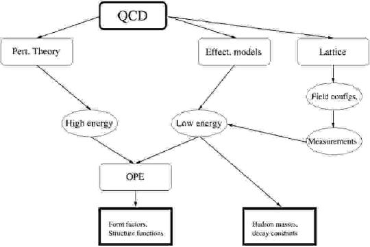
Figure 7: Different methods for obtaining prediction in QCD.

6 Discretization

As discussed in 3, for the construction of a quantum field theory on a lattice, the functional $S[\varphi(x)]$ is required. This functional should reduce to the Euclidean action $\mathscr{S}[\varphi(x)]$ in the continuum limit and for differentiable paths. Before applying the limit prescription, it will thus differ by ${\cal O}(a)$-effects from the continuum expression — meaning that in general the choice of $S[\varphi(x)]$ is not unique but still leaves freedom to choose all terms of order ${\cal O}(a^{n})$ with $n\geq 1$. This freedom should be used to find the form best suited for numerical calculations.

1 Scalar Fields

Consider the complex field $\phi(x)$ defined on the sites $x\in\mathbb{Z}^{4}_{\Omega}$. The continuum Lagrangian corresponding to this situation is given by Eq. (6). One candidate for the lattice version of the action is then given by [24]:

$$S[\phi(x)]=\sum_{x}\left(\sum_{\mu=0}^{3}\phi(x)^{\dagger}\phi\left(x+\hat{\mu}\right)+m^{2}\phi(x)^{\dagger}\phi(x)+V[\phi(x)]\right)\,.$$ (64)

There are certainly other ways to replace the derivative, but the present choice is the simplest way to incorporate neighbor fields. Consequently, this choice is suitable for numerical investigations and will be used in this thesis.

A particularly interesting model is the so-called $\phi^{4}$-model, where one sets

$$V[\phi]=\frac{\lambda}{4!}\phi^{4}\,.$$

This model appears to be an interacting, nontrivial field theory at first sight, but already early it has been conjectured [31] that it might only give rise to a non-interacting theory of free particles. In later investigations this surmise has been corroborated [91, 92]. However, a rigorous proof is still missing.

2 Gauge Fields

In the continuum form (57), the gauge field is given in terms of parallel transporters along infinitesimal distances. By putting the system on a lattice, the shortest (non-zero) distance is the lattice spacing $a$. The parallel transporter connecting a point $x\in\mathbb{Z}^{4}_{\Omega}$ with its neighbor $x+\hat{\mu}$ is denoted by $U(x,x+\hat{\mu})$. It is an element of SU$(N)$. The simplest gauge-invariant object one can construct is a closed loop with a side length of one lattice unit usually called the plaquette. Starting from the point $x\in\mathbb{Z}^{4}_{\Omega}$, one can construct the plaquette lying in the $\mu\nu$-plane by considering

$$U_{\mu\nu}(x)=U(x,x+\hat{\mu})U(x+\hat{\mu},x+\hat{\mu}+\hat{\nu})U(x+\hat{\mu}+\hat{\nu},x+\hat{\nu})U(x+\hat{\nu},x)\,.$$ (65)

Due to the fact that $U(x,x+\hat{\mu})=U^{\dagger}(x+\hat{\mu},x)$ one can rewrite (65):

$$U_{\mu\nu}(x)=U(x,x+\hat{\mu})U(x+\hat{\mu},x+\hat{\mu}+\hat{\nu})U^{\dagger}(x+\hat{\nu},x+\hat{\mu}+\hat{\nu})U^{\dagger}(x,x+\hat{\nu})\,.$$ (66)

The suggestion of Wilson [93] was to use real part of the trace of $U_{\mu\nu}$ summed over all plaquettes as the action of the system,

$$S_{\mbox{\tiny g}}[U(x)] = -\beta\frac{1}{2\mbox{Tr}\,\mathbf{1}}\sum_{x}\sum_{\mu<\nu}\left(\mbox{Tr}\,U_{\mu\nu}(x)+\mbox{Tr}\,U_{\mu\nu}^{-1}-1\right)$$ (67)

$$= \beta\sum_{x}\sum_{\mu\nu}\left(1-\frac{1}{N}\mbox{Re}\,\mbox{Tr}\,U_{\mu\nu}(x)\right)\,,$$

which is the discretized form of the non-Abelian gauge field part in Eq. (57). This form, however, is also applicable to the case of Abelian gauge fields with the Lagrangian given by Eq. (9).

For later applications, the more convenient notation $U_{\mu}(x)\equiv U(x,x+\hat{\mu})$ will be used from now on; hence, the plaquette, Eq. (66), is written as

$$U_{\mu\nu}(x)=U_{\mu}(x)U_{\nu}(x+\hat{\mu})U^{\dagger}_{\mu}(x+\hat{\nu})U^{\dagger}_{\nu}(x)\,.$$ (68)

The path integral form of the partition function, Eq. (39), on a finite lattice $\mathbb{Z}^{4}_{\Omega}$ is given by

$$Z=\int\prod_{x}dU(x)\exp\left[-S[U(x)]\right]\,,$$ (69)

where the measure $dU(x)$ is the Haar measure on the gauge group (see App. 8.A).

One of the properties of the Haar measure is that the total integral over the group space on a single lattice point $x$ is finite. Thus, any gauge-fixing procedure is unnecessary [24]. However, if one attempts to apply a saddle-point approximation to (69) (see Sec. 3), the presence of zero modes will spoil the inverse of the two-point function [35]. This requires the introduction of a gauge fixing procedure and auxiliary fields known as Faddeev-Popov ghosts [35].

It is important to point out that the entire partition function (69) is manifestly gauge invariant since it is composed of gauge invariant loops $U_{\mu\nu}(x)$ only. It can be shown [46, 24] that it is impossible to break gauge invariance spontaneously. This fact implies that the expectation value of the $U_{\mu}(x)$ will always vanish, a fact which is also known as the Elitzur theorem:

$$\langle U_{\mu}(x)\rangle=0\,.$$

Eq. (67) has two limits, where the form of the gauge fields can be written down explicitly: If one considers $\beta\rightarrow 0$, the situation resembles the hot temperature limit in thermodynamics. Thus, the resulting gauge field configurations are called hot configurations — the values of the gauge field variables are arbitrary and they can take any random values from their domain of definition. The limit $\beta\rightarrow\infty$, is referred to as the zero-temperature limit. The correlation between neighbor points increases, therefore the total correlations length will increase. Finally, the values of the field variables are given by $U_{\mu}(x)=1\ \forall x\in\Omega$. If the system undergoes a second order phase transition, i.e. if the correlation length diverges, this describes the continuum quantum field theory.

3 D-Theory

There exists also a discretization technique entirely different from the methods discussed in Sec. 2. It is based on a quantum link model, which is constructed in such a way that it is still locally gauge invariant and should thus reduce to the correct continuum form of the Yang-Mills theory, just as (67) is expected to do. Quantum link models with local gauge invariance have been formulated by Horn in [94] for the first time, where a model with a local SU$(2)\otimes$U$(1)$ gauge invariance has been formulated. They have been extended to the case of SU$(N)$ by Orland and Rohrlich in [95]. These models, however, did not yet relate to the quantum field theories with continuous symmetries as discussed in this thesis. Only recently it has been realized by Chandrasekharan and Wiese in [96], how one can relate the discrete quantum link models with continuum field theories. For a review of the ingredients of quantum link models see [97].

Globally Symmetric Models

The basic ideas behind the construction of D-theory become clear if one considers a spin model, namely the O$(3)$-model in two space dimensions. The action is given by (cf. (67))

$$S[\vec{s}]=-\frac{1}{g}\sum_{x}\sum_{\mu}\vec{s}(x)\cdot\vec{s}(x+\hat{\mu})\,,$$ (70)

with $\vec{s}(x)$, $x\in\mathbb{Z}^{2}_{\Omega}$, being three-component unit vectors. The coupling constant is given by $g$. After quantizing this spin system (cf. Sec. 3) by considering the partition sum

$$Z=\int[\mbox{d}\vec{s}]\exp\left[-S[\vec{s}]\right]\,,$$ (71)

one arrives at a model which is asymptotically free and has a non-perturbatively generated mass-gap. The question arises, whether it is possible to find a different lattice system (with no resemblance to Eq. (70)) which still reduces to the same continuum field theory in the sense discussed in Sec. 3. This construction is indeed possible and can be done as follows:

1. Replace the classical vectors $\vec{s}(x)$ by quantum spin operators $\hat{S}(x)$ which are elements of the algebra $\hat{S}(x)\in\mbox{su}(2)$, i.e. they are the generators of the SU$(2)$-group (cf. Appendix 8.C).

2. Replace the classical action (70) by the Hamiltonian

   $$\hat{H}=J\sum_{x}\sum_{\mu}\hat{S}(x)\cdot\hat{S}(x+\hat{\mu})\,,$$ (72)

   which yields the quantum Heisenberg model. The partition sum (71) is therefore replaced by the state sum

   $$Z=\mbox{Tr}\,\exp\left[-\beta H\right]\,.$$ (73)

   It is important to point out that the particular representation of the group is not important — the trace can be taken over any representation, although in practice one usually adopts the fundamental representation [97]. In the following, the discussion is restricted to the case $J>0$, i.e. the anti-ferromagnetic Heisenberg system.

3. By using a Suzuki-Trotter discretization, the state sum (73) becomes a partition function of a three-dimensional model with continuous symmetry with a certain lattice spacing $a_{3d}$. This model is invariant under a global SO$(3)$-symmetry since the Hamiltonian (72) is also invariant. The low-energy properties of the resulting model can be described using chiral perturbation theory [98]. The symmetry is spontaneously broken in the ground state, resulting in two Goldstone bosons which are represented by fields in the coset SO$(3)$/SO$(2)=S^{2}$. Thus, they describe the same kind of three-component unit vectors which appear in the original action, Eq. (70). The low-energy effective action of the Goldstone bosons can be formulated using chiral perturbation theory:

   $$S[\vec{s}]=\int_{0}^{L_{0}}\int d^{2}x\;\frac{\rho_{2}}{2}\left(\partial_{\mu}\vec{s}\cdot\partial^{\mu}\vec{s}+\frac{1}{c^{2}}d_{0}\vec{s}\cdot d^{0}\vec{s}\right)\,,$$ (74)

   with $L_{0}$ being the extend of the third dimension which has been introduced by the Suzuki-Trotter discretization. The parameters $c$ and $\rho_{s}$ constitute the spin-wave velocity and the stiffness, respectively.

4. Finally, there exists a mapping of the two systems, which has been suggested by Hasenfratz and Niedermayer [99]. This is achieved by a block spin transformation, which maps subvolumes of size $\Omega_{\mbox{\tiny sub}}=L_{0}\times(L_{0}c)^{2}$ to a new lattice system. The new lattice will then have a lattice spacing given by $a_{2d}=L_{0}c$ and the coupling constant $g$ of the transformed system is given by

   $$1/g=L_{0}\rho_{s}+{\cal O}(1/(L_{0}\rho_{s}))\,.$$ (75)

   Thus, the continuum limit of the new lattice model is obtained in the limit $L_{0}\rightarrow\infty$. The correlation length (and thus the inverse mass scale of the system) is given in terms of $L_{0}$ by

   $$\xi=\frac{ec}{16\pi\rho_{s}}\exp\left(2\pi L_{0}\rho_{s}\right)\left(1-\frac{1}{4\pi L_{0}\rho_{s}}+{\cal O}(1/(L_{0}\rho_{s})^{2})\right)\,.$$ (76)

   In the limit $L_{0}\rightarrow\infty$, the correlation length thus diverges exponentially and the extent $L_{0}\ll\xi$ becomes negligible and hence the system undergoes dimensional reduction.

In conclusion, one can say that D-theory introduces a substructure to the original system. The lattice spacing of this substructure is much smaller than the corresponding lattice spacing of the original theory. However, the resulting lattice action is obtained from exact blocking of the continuum fields, implying that the lattice artifacts are of order ${\cal O}(a_{3d})$. This means that in practical simulations, one can use lattice spacings of the same order of magnitude as with the Wilson discretization and the resulting theory has a lattice spacing $a_{2d}\gg a_{3d}$.

Models with Local Gauge Symmetries

The construction principle underlying D-theory can be applied to other models as well. The important cases of U$(1)$ and SU$(2)$ gauge theories have been discussed in [96]. The application to the case of QCD has been considered in [100]. For a review consult [101].

In [102], it has been conjectured how the parameter space of the D-theory formulation is related the coupling of the conventional theory. Also the principal chiral model could have been formulated in this way and has been shown to reduce to the conventional discretization formulation [103]. From these discussions it becomes clear that in fact D-theory is an alternative formulation of the discretization of quantum field theories with local gauge symmetries.

Simulation Algorithms

For the simulation of quantum spin systems, a particular efficient class of algorithms is available, known as cluster algorithms. While the most efficient algorithms to be discussed in Chapter 2 which are applicable to the Wilson action Eq. (67) are all local, the cluster algorithms are global.

Cluster algorithms have first been introduced to quantum spin systems by Swendsen and Wang in [104]. These algorithms exploit the mapping introduced by Fortuin and Kasteleyn [105] to rewrite the partition function and to formulate a global algorithm which is able to flip a large cluster of spins at once. In this way, critical slowing down which will be discussed in Sec. 4 is effectively reduced, provided the average cluster size scales proportional to the correlation length of the system. For a general overview of cluster algorithms see [106]. A useful generalization of cluster algorithms which might be applicable to D-theory is given by the world-line Monte-Carlo algorithms, see [107, 108, 109] and [110] for a new implementation.

If indeed locally gauge symmetric models can be simulated efficiently using a quantum spin system, the inclusion of dynamical fermions would be straightforward [97]. Thus, full Yang-Mills theory might be efficiently simulated. There is furthermore reason to believe, that the fermionic sign problem for a discussion) may be handled better in the framework of quantum spin systems. For an overview see [111]. For further readings consult [112].

This benefit could then be used to overcome the limitations of current algorithms regarding the sign of the fermionic determinant. This problem occurs whenever an odd number of dynamical fermion flavors is being simulated very close to massless fermion flavors. This point will be discussed in Secs. 4 and 3.

4 Fermion Fields

The Euclidean space version of (54) is given by

$$\mathscr{L}(\Psi_{N},\bar{\Psi}_{N},A^{\mu}_{a})=\bar{\Psi}_{N}\left(/\!\!\!\!D-m\right)\Psi_{N}\,,$$ (77)

where the $\gamma_{\mu}$-matrices in Euclidean space must be employed, cf. App. 7.A. The representation of Eq. (77) on the lattice is a very complicated task. As shown in App. 8.F, the basic fields $\bar{\Psi}(x),\Psi(x)$ are elements of a Grassmann algebra. These fields admit a representation as four-component vectors with the choice of $\{\gamma_{\mu}\}$ as given in App. 7.A. Thus, the task of putting an $N$-component Yang-Mills field in Euclidean space, on the lattice is equivalent to finding a matrix $Q_{ab,\mu\nu}(y,x)$ with $a,b=1,\dots,N$, $\mu,\nu=0,\dots,3$, and $x,y\in\mathbb{Z}^{4}_{\Omega}$, giving rise to the action

$$S_{\mbox{\tiny f}}=-\sum_{xy}\sum_{ab,\mu\nu}\bar{\Psi}^{a\mu}(y)Q_{ab,\mu\nu}(y,x)\Psi^{b\nu}(x)\,.$$ (78)

To simplify the notation, the indices $a,b$, and $\mu,\nu$ will be suppressed from now on. The corresponding path integral defining the quantum partition function, Eq. (39), is then given by (cf. Eq. (23) in App. 3)

$$Z=\int[\mbox{d}\bar{\psi}][\mbox{d}\psi]\exp\left[-\sum_{xy}\bar{\Psi}(y)Q(y,x)\Psi(x)\right]=\det{Q}\,.$$ (79)

For the discretization of the fermionic action, a number of choices is available. However, the Nielsen-Ninomiya theorem [113, 114] puts a general limit on any lattice fermion action; under some natural assumptions on the lattice action, it follows that there is an equal number of left- and right-handed particles for every set of quantum numbers.

This implies that on the lattice the fermion spectrum consists of pairs of fermions and fermion-mirrors. Thus, apparently it appears to be impossible to implement the structure of Dirac fermions on a discrete space-time. However, one can evade the physical consequences by decoupling the superfluous fermion states. In QCD this can be achieved, for instance, by giving the fermion doublers a mass proportional to the cut-off $a^{-1}$. This procedure, however, does not work in a chirally symmetric model; in fact, it is a general consequence of the topological character of lattice theory that there does not exist a regularized chiral fermion theory that has the following properties (see for a proof of this no-go theorem [115]):

1. global invariance under the gauge group,

2. a different number of left- and right-handed species for given charge combinations,

3. the (correct) Adler-Bell-Jackiw anomaly,

4. and an action bilinear in the Weyl field.

The absence of the Adler-Bell-Jackiw anomaly displays the fact that the axial U${}_{A}(1)$ current is conserved because of the cancellation of opposite-handed species.

Of course, in the continuum formulation any gauge invariant regularization scheme yields the same expression for the axial anomaly. Thus, this should also be valid for the lattice regularization, too. Consequently, any candidate for the lattice discretization of gauge theories should reproduce the axial anomaly in the continuum limit. Indeed it has been shown in [116] that the Wilson discretization [117] does reproduce the chiral anomaly in the continuum limit. The Wilson action breaks chiral symmetry on the lattice explicitly thus removing the unwanted doublers from the propagators. The chiral symmetry breaking term is actually an irrelevant contribution to the lattice Ward identity, i.e. it is proportional to the lattice spacing, $a$. However, it does not disappear in the limit $a\rightarrow 0$, but rather accounts precisely for the anomaly. For a discussion of the phase structure associated with Wilson fermions on the lattice consult [118].

A theorem showing that, under the rather general conditions of locality, gauge covariance and the absence of species doubling, the lattice action gives rise to the axial anomaly has been given in [119, 120] for Abelian gauge theories and generalized to the case of QCD (which can in principle be generalized to any non-Abelian gauge theory) in [121]. However, the axial flavor mixing current should be non-anomalous. That this is indeed the case has been shown in [122]. The proofs have all been done perturbatively on the lattice using the expansion from [123].

The problem of representation of chiral symmetry on the lattice has been resolved only recently, when it was realized that a solution of the Ginsparg-Wilson relation (GWR) introduced in [124] has an exact chiral symmetry on the lattice, as has first been discussed in [125]. The first fermionic action which actually satisfies the GWR was the perfect action of [126]. For practical purposes, the solution of Neuberger [127, 128] is the most widely used today (for a historical overview of the development leading to the Neuberger representation, see [129]). Finally it is important to point out that the theorem in [121] also applies to Ginsparg-Wilson fermions thus ensuring that they reduce to the correct fermionic action in the continuum limit.

However, since the numerical effort for the evaluation of Neuberger fermions increases by $1-2$ orders of magnitude compared to Wilson fermions, the calculation with dynamical Neuberger fermions is still prohibitively expensive.

As argued above, the Wilson action breaks chiral symmetry on the lattice with a term of order ${\cal O}(a)$. Thus, the action depends linearly on the cutoff and physical observables might show sizable lattice artifacts when approaching the continuum limit. As has been put forward by Sheikholeslami and Wohlert in [130] the cancellation of the ${\cal O}(a)$ dependence can be calculated perturbatively up to a prefactor, the parameter $c_{\mbox{\tiny SW}}$. Observables computed using this fermionic action with a non-perturbatively calculated $c_{\mbox{\tiny SW}}$ indeed show weaker artifacts with an ${\cal O}(a^{2})$-dependence as has been demonstrated in e.g. [131, 132]. This program is also called clover-improvement, since the perturbative correction has the shape of a four-leaf clover. Clover-improvement turned out to be useful in a number of studies employing the hybrid Monte-Carlo (HMC) algorithm (see Sec. 2). When applying it to multiboson (MB) algorithms (cf. Sec. 3), however, the required local staples (see App. 9) would soon become extremely complicated and the merits of the improvement might become obscured by the increased algorithmic demands.

Since the major focus of this thesis lies on Wilson fermions, a few words about its explicit breaking of chiral symmetry are in order. Having no chiral symmetry means that there is explicit symmetry breaking by the non-chiral fermion mass. Thus, the physics of spontaneous chiral symmetry breaking may be shadowed. In fact, it turns out to be extremely difficult to perform lattice calculations with light quarks since the numerical effort increases polynomially in the inverse quark mass [133]. However, when performing the continuum limit at sufficiently small quark masses (where the precise meaning of “sufficient” can only be given very roughly within $\chi$PT [10]), one can afterwards extrapolate to the desired quark mass and still be able to extract correct continuum physics from numerical lattice simulations. This is the method usually adopted in actual calculations employing light fermions.

With the conventions used in this work, the Wilson action for a single fermion flavor reads:

$$S_{\mbox{\tiny f}}=\sum_{xy}\Psi(y)^{\dagger}Q(y,x)\Psi(x)\,,$$ (80)

where the Wilson matrix $Q(y,x)$ is defined to be

$$Q(y,x) = \displaystyle\delta(y,x)-\kappa\sum_{\rho=0}^{3}\Bigl{(}U_{\rho}\left(y-\hat{\rho}\right)\left(1+\gamma_{\rho}\right)\delta\left(y,x+\hat{\rho}\right)$$ (81)

$$\displaystyle\phantom{\delta(y,x)-\kappa\sum}+U_{\rho}^{\dagger}(y)\left(1-\gamma_{\rho}\right)\delta\left(y,x-\hat{\rho}\right)\Bigr{)}\,,$$

with $\kappa$ being a function of the bare mass parameter which is called hopping parameter. Due to the anticommutivity of the fermion field, one also has to include antiperiodic boundary conditions in the coupling to the gauge field, see [24] for a thorough discussion. This usually proceeds by choosing all $U_{0}(x)\rightarrow-U_{0}(x)$, with $x$ restricted to a single timeslice when applying the matrix multiplication with (81). This sign is not explicitly written here. For the local form to be discussed in App. 9, however, it is necessary to treat this factor separately.

The matrix $Q(y,x)$ in (81) consists of the local $\delta$-function contribution and a “derivative” term containing nearest-neighbor interactions. This is often called the hopping matrix, $D(y,x)$, and can be considered to be the lattice version of the covariant derivative in the continuum Dirac matrix Eq. (54), $/\!\!\!\!D$. The “mass” has been taken to unity and the hopping parameter $\kappa$ has been written in front of the lattice derivative term which can be achieved by a redefinition of the fields $\Psi$. Thus, the Wilson matrix explicitly breaks chiral symmetry on the lattice. As will soon become clear, one can nonetheless recover the correct chiral behavior by fine-tuning the $\kappa$ parameter. In terms of the hopping matrix, Eq. (81) can be written as

$$Q(y,x) = \displaystyle\delta(y,x)-\kappa D(y,x)\,,$$

$$D(y,x) = \displaystyle\sum_{\rho=0}^{3}\Bigl{(}U_{\rho}\left(y-\hat{\rho}\right)\left(1-\gamma_{\rho}\right)\delta\left(y,x+\hat{\rho}\right)$$ (82)

$$\displaystyle\phantom{\delta(y,x)-\kappa\sum}+U_{\rho}^{\dagger}(y)\left(1-\gamma_{\rho}\right)\delta\left(y,x-\hat{\rho}\right)\Bigr{)}\,.$$

The Wilson matrix, $Q(y,x)$, fulfills the $\gamma_{5}$-hermiticity property

$$Q^{\dagger}(y,x)=\gamma_{5}Q(y,x)\gamma_{5}\,,$$ (83)

as can be seen from inspection. This leads to the following properties: the eigenvalues are either real or come in complex conjugate pairs. If one takes the determinant of $Q(y,x)$, it can therefore only change sign if an odd number of purely real eigenvalues becomes negative. At this point it should also be remarked that the total number of real eigenvalues is in the continuum related to the topological charge via the Atiyah-Singer-index theorem [51]. For an investigation of the validity of the index theorem on the lattice see [134, 135].

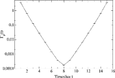
Figure 9: Symmetrized correlation function for the vector meson with three dynamical fermions at $\beta=5.2$ and $\kappa=0.156$.

The spectrum of the hopping matrix $D(y,x)$ in Eq. (4) has been examined in [136]. For recent overviews and results obtained from eigenvalue methods, see [137, 138, 139]. In general, the following picture emerges: For a configuration with $\beta=0$ (cf. Eq. (67)), the spectrum fills a disc centered at the origin with radius two (see Fig. 8). In the small coupling regime, the structure is more complicated (consult Fig. 9): The outer shape of the eigenvalues forms an ellipse which has a large radius of eight and a small radius of four. However, four circles with radius two each, centered on the real axis, are left out. At intermediate values of $\beta$, one finds spectra interpolating between these two situations: the spectrum starts to spread and the holes start to form, but the eigenvalue density is not yet completely zero in the holes. Especially, the real eigenvalues tend to populate the bulks for a rather long time compared to the imaginary ones (see [134]). When measuring the lattice spacing in physical units, $a$, one finds that ${\cal O}(a)$ effects manifest themselves prominently in the real eigenvalues still lying in the holes [134].

Considering then the complete Wilson matrix, $Q(y,x)$, one finds that the lower bound of the spectrum becomes zero if (in the free case) $\kappa_{\mbox{\tiny free}}=1/8$. A derivation of this result for free configurations can also be found in [24]. In this case, the Wilson matrix describes massless Dirac fermions. This point is called the chiral point and the associated value of $\kappa$ is called the critical value $\kappa_{\mbox{\tiny crit}}$.

Hence, if $\beta$ increases from zero to $\infty$, the values of $\kappa_{\mbox{\tiny crit}}$ decrease from $\kappa_{\mbox{\tiny crit}}=1/4$ down to $\kappa_{\mbox{\tiny crit}}=\kappa_{\mbox{\tiny free}}$. For practical determinations of $\kappa_{\mbox{\tiny crit}}$, see Sec. 2.

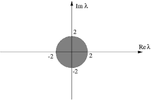
Figure 8: Spectrum of the hopping matrix, $D(y,x)$ in Eq. (4), in the limit $\beta\rightarrow 0$.

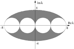
Figure 9: Spectrum of the hopping matrix, $D(y,x)$ in Eq. (4), in the limit $\beta\rightarrow\infty$.

The Wilson matrix given in equation (4) is not only non-Hermitian, it is even non-normal, i.e.

$$[Q(y,x),Q^{\dagger}(y,x)]\neq 0\,.$$

Thus, it cannot be diagonalized by a unitary matrix; however, it is possible to diagonalize the Wilson matrix by a similarity transformation with non-unitary matrices,

$$\mathbf{Q}=S^{-1}\cdot Q\cdot S\,.$$ (84)

A further consequence of non-normality is that $Q(y,x)$ will in general have different left- and right eigenvectors [140], a property which should be respected in the definition of matrix elements in terms of the eigenvectors [66, 141]. In several cases (as it is the case for the sampling algorithms to be discussed in Chapter 2), one only needs the determinant $\det{Q}$. Therefore it is often convenient to use the Hermitian variant of the Wilson action which can be obtained by replacing the matrix $Q(y,x)$ by the Hermitian Wilson matrix $\tilde{Q}(y,x)$:

$$\tilde{Q}(y,x)=\gamma_{5}Q(y,x)\,.$$ (85)

It is easy to show that $\tilde{Q}(y,x)$ is in fact self-adjoint:

$$\tilde{Q}^{\dagger}(y,x) = Q^{\dagger}(y,x)\gamma_{5}$$

$$= \gamma_{5}Q(y,x)=\tilde{Q}(y,x)\,.$$

The spectrum of $\tilde{Q}(y,x)$ is more complicated than the spectrum of $Q(y,x)$ and determining the sign of the determinant is a non-trivial task. Exploiting the fact that $\det\gamma_{5}=1$, one can, however, always use

$$\det\tilde{Q}=\det Q\,.$$

Even-Odd Preconditioning

A simple transformation allows the Wilson action to be rewritten [142, 143] such that the condition number is reduced. To do this we divide the lattice into two distinct subsets of “even” and “odd” coordinates:

Even-odd splitting:

If the coordinates of a given lattice site are given by $\left(t,x,y,z\right)\in\Omega$ then a point belongs to the “odd” subset iff

$$\left(t+x+y+z\right)\ \mathop{mod}\ 2=1.$$

Otherwise they belong to the “even” subset.

If we rearrange the components of the vector in (81) in such a way that the color spinor is given by $\left(\phi_{\mbox{\tiny even}},\phi_{\mbox{\tiny odd}}\right)$ with the first half being “even” sites and the second half “odd” sites, then the Wilson matrix (81) takes the following shape:

$$\tilde{Q}(y,x)=\gamma_{5}\left(\begin{array}[]{cc}1&-\kappa D_{eo}\\ -\kappa D_{oe}&1\end{array}\right)\,.$$ (86)

Using the Schur decomposition [144]

$$\det\left(\begin{array}[]{cc}A&B\\ C&D\end{array}\right)=\det A\;\det\left(D-CA^{-1}B\right)\,,$$ (87)

one arrives at the preconditioned action

$$\hat{Q}=\gamma_{5}\left(1-\kappa^{2}D_{oe}D_{eo}\right)\,.$$ (88)

Since this matrix has the same determinant as (81) it yields the same action (80). However, the smallest eigenvalue is about a factor of two larger, making the inversion simpler. On the other hand, (88) has a more complicated shape (it now contains next-to-nearest neighbor interactions). Therefore the total effort for a matrix multiplication stays the same, but the memory requirement for a color spinor has been reduced.

5 Yang-Mills Theory

Finally, one can write down the total discretized form of the continuum Yang-Mills action whose Lagrangian is given in Eq. (57):

$$S_{\mbox{\tiny g+f}} = \beta\sum_{x}\sum_{\mu\nu}\left(1-\frac{1}{N}\mbox{Re}\,\mbox{Tr}\,U_{\mu\nu}(x)\right)+\sum_{xy}\Psi(y)^{\dagger}Q(y,x)\Psi(x)$$ (89)

$$= S_{\mbox{\tiny g}}+\ln\det Q(y,x)\,,$$

with $Q(y,x)$ being the Wilson matrix (81). The bare mass parameter $\kappa$ appearing in $Q(y,x)$ refers to the contribution of dynamical sea quarks (i.e. the virtual quark loops). It is therefore termed $\kappa_{\mbox{\tiny sea}}$. The evaluation of the determinant becomes increasingly difficult as $\kappa_{\mbox{\tiny sea}}$ approaches $\kappa_{\mbox{\tiny crit}}$, whose precise value can only be determined non-perturbatively (see Sec. 2). Since the evaluation of the determinant of such a huge matrix is highly difficult, it is sometimes being set equal to one (which corresponds to $\kappa_{\mbox{\tiny sea}}=0$), resulting in the fermionic contribution to (89) being totally absent. If this is only being done in the generation of configurations (i.e. the ensemble is sampled with the pure gauge action) this amounts to removing the contributions of sea quarks. This defines the quenched approximation mentioned in Sec. 3.

Chapter 2 Numerical Methods

In this chapter, the numerical methods are introduced which are required to simulate lattice gauge theories with and without dynamical fermion contributions.

The properties of Monte-Carlo algorithms are introduced in Sec. 1. They make use of Markov chains, as it will be explained in Sec. 1.

Section 2 introduces into the subject of time series analysis, in particular the analysis of autocorrelations in a Monte-Carlo time series.

The measurement of hadronic masses is discussed in Sec. 3.

The particular algorithms used for the Monte-Carlo integration scheme are given in Secs. 4 and 5. The former concentrates on the algorithms required for scalar and gauge fields, while the latter introduces algorithms applicable to simulations with dynamical fermionic contributions. The most important bosonic algorithms are the Metropolis algorithm (Sec. 1), the heatbath algorithm (Sec. 2) and the overrelaxation technique (Sec. 3).

The algorithms for sampling contributions of dynamical fermions are treated in Sec. 5. First the general problems one encounters when evaluating the determinant of the Wilson matrix are introduced in Sec. 1. It will become clear, that any algorithm dealing with the fermionic determinant requires the inversion of a large matrix describing the contribution of the discretized fermionic degrees of freedom. Then the most widely used algorithm for the simulation of dynamical fermion flavors, the hybrid Monte-Carlo (HMC) algorithm, is reviewed in Sec. 2.

In this thesis, however, a more advanced algorithm for this subject will be used, namely a variant of the multiboson (MB) algorithms. This class of algorithms is discussed in Sec. 3. These algorithms are able to overcome several limitations and shortcomings of the HMC, but at the cost of far more complexity.

As has been mentioned above, matrix inversion is an essential tool for the implementation of fermion algorithms. The tools required for the implementation of matrix inversion algorithms are described in Sec. 6. The inversion algorithms presented are static algorithms in Sec. 1, the Conjugate-Gradient iteration (Sec. 2), the GMRES algorithm (Sec. 3), and the BiCGStab scheme (Sec. 4).

Finally, the tools for the computation of eigenvalues of matrices are shortly reviewed in Sec. 7. They are important for the application of static matrix inversion schemes and thus for the implementation of multiboson algorithms.

1 Monte-Carlo Algorithms

The path integral definition introduced in Sec. 3 allows for an evaluation using ensembles of field configurations as discussed in Sec. 4. This definition, however, requires to perform an integration on an infinite space of operator-valued distributions $\{{\phi}\}$ with a given probability distribution $\rho\{{\phi}\}$ and a measure $[\mbox{d}\phi]$. An approach different to the reformulation in terms of Gaussian integrals discussed in Sec. 3 is the application of a numerical integration using a Monte-Carlo scheme. That such an endeavor can indeed yield physical results in quantum field theories was first demonstrated in [145, 6]. In this section it will be demonstrated how an algorithm can be designed in such a way that it generates a finite set of independent gauge field configurations which can be used as an estimator to the ensemble averages and thus to the path integral (40).

A Monte-Carlo integration algorithm is an algorithm which computes a finite set of mesh points and yields a statistical approximation $\bar{A}\approx\langle\hat{A}\rangle$ to the given problem. The error of the approximation is given by the statistical error of the integration scheme. To be specific, let’s consider an algorithm which generates a finite sequence $[\phi_{n}]$, $n=1,\dots,N$, of $N$ statistically independent configurations. These must be distributed according to the probability density $\rho\{{\phi}\}$ of the underlying ensemble. The finite sequence is called the sample of configurations. If they have been taken randomly from the ensemble (46), the sample average

$$\bar{A}=\frac{1}{N}\sum_{n=1}^{N}e^{-S\left[\phi_{n}\right]}\hat{A}\left[\phi_{n}\right]$$ (1)

is an estimator for the ensemble average $\langle\hat{A}\rangle$ with an error given by the variance of the statistical estimate (40). Consequently, the error of the Monte-Carlo integration behaves as $1/\sqrt{N}$. This is different from the standard integration schemes like Simpson’s rule [44] whose error behaves as $N^{-4/d}$, with $d$ being the dimension of the underlying space. Obviously this method is better for low dimensions (for $d<8$) and worse for higher dimensions ($d>8$). There are better algorithms than Simpson’s rule, but none is competitive with Monte-Carlo integrations in very large dimensions. On the other hand, no Monte-Carlo integration is competitive with deterministic algorithms at lower dimensions.

It is obvious how to generalize Eq. (1) if the sample configurations have been drawn from the canonical ensemble (48). Then the estimator is given by the sample average

$$\bar{A}=\frac{1}{N}\sum_{n=1}^{N}\hat{A}\left[\phi_{n}\right]\,.$$ (2)

Since such an integrand may be peaked rather narrowly around its average value, the sampling algorithm should generate only the relevant contributions. Such a procedure is called importance sampling.

In the following, the theoretical basis needed to design Monte-Carlo algorithms from Markov chains is founded.

1 Markov Chains

An important concept for the design of an algorithm yielding the desired sample of configurations is the Markov chain:

Markov chain:

A Markov chain $\left([\phi],\tilde{\rho}[\phi],{\cal P}\right)$ consists of a set of states $[\phi_{n}]$ defined on a base space. For the purposes in this thesis, this is the space of discretized fields, $\mathbb{Z}^{4}_{\Omega}$. A specific element $\phi_{i+1}$ is generated from the previous element $\phi_{i}$ by a stochastic process ${\cal P}$:

$$\phi_{i+1}={\cal P}\phi_{i}\,.$$

The associated transition probability is given by the matrix element ${\cal P}\left([\phi_{i}]\rightarrow[\phi_{i+1}]\right)$. It solely depends on the state $\phi_{i}$. The Markov density $\tilde{\rho}[\phi]$ is a unit vector in the state space spanned by all $\phi$, in which the matrix ${\cal P}\left([\cdot]\rightarrow[\cdot]\right)$ acts.

If the states $[\phi_{n}]$ have the probability distribution $\tilde{\rho}[\phi]$, applying ${\cal P}$ once to the end of the chain may change the probability distribution. With the initial distribution given by $\tilde{\rho}_{n}[\phi]$, one obtains a new distribution $\tilde{\rho}_{n+1}[\phi]$ via

$${\cal P}\tilde{\rho}_{n}[\phi]=\sum_{\{\phi_{i}\}}{\cal P}\left([\phi_{i}]\rightarrow[\phi]\right)\tilde{\rho}_{n}[\phi_{i}]=\tilde{\rho}_{n+1}[\phi]\,.$$

Using this language one can define the following notions related to Markov chains:

Irreducibility:

Denote $\phi_{j}={\cal P}^{(M)}\phi_{i}$ for $M$ repeated applications of ${\cal P}$ on $\phi_{i}$, yielding $\phi_{j}$. A chain is called irreducible if for any states $\xi,\zeta\in\mathbb{Z}^{4}_{\Omega}$, there exists an $M\geq 0$ such that

$$\zeta={\cal P}^{(M)}\xi\,.$$

Aperiodicity:

Define $p_{ij}^{(M)}={\cal P}\left([\phi_{i}]\rightarrow[\phi_{i+1}]\right)\dots{\cal P}\left([\phi_{j-1}]\rightarrow[\phi_{j}]\right)$ to be the $M$-step transition probability to reach $\phi_{j}$ from the starting element $\phi_{i}$ in $M$ steps. A chain is called irreducible and aperiodic if for each pair $\phi_{i},\phi_{j}\in\mathbb{Z}^{4}_{\Omega}$ there exists an $M_{0}=M_{0}\left(\phi_{i},\phi_{j}\right)$ such that $p_{ij}^{(M)}>0$ for all $M\geq M_{0}\left(\phi_{i},\phi_{j}\right)$.

Recurrence time:

Take a state $\xi\in\mathbb{Z}^{4}_{\Omega}$. Let $\left({\cal P}\left([\xi]\rightarrow[\xi]\right)\right)^{(M)}$ be the probability to reach $\xi$ after $M$ applications of ${\cal P}$ on $\xi$. Then the mean recurrence time $\tau_{\xi}$ is given by

$$\tau_{\xi}=\sum_{M=1}^{\infty}M\left({\cal P}\left([\xi]\rightarrow[\xi]\right)\right)^{(M)}\,.$$

Positivity:

A state $\xi\in\mathbb{Z}^{4}_{\Omega}$ is called positive iff $\tau_{\xi}$ is finite.

Stationary distribution:

A probability distribution $\tilde{\rho}[\phi]$ is called stationary distribution of the Markov chain if it stays invariant under application of ${\cal P}$:

$$\tilde{\rho}[\phi]={\cal P}\tilde{\rho}[\phi]\,.$$

A particularly important class of Markov chains is given by the irreducible, aperiodic chains whose states are positive [32, 44]. Indeed one can prove the following theorem:

Existence and uniqueness of the stationary point:

Take an irreducible, aperiodic Markov chain with positive states $[\phi_{n}]$ and transition function ${\cal P}$. Hence, the chain has the starting distribution $\tilde{\rho}[\phi_{n}]$. Then the limiting probability distribution $\tilde{\rho}_{\mbox{\tiny Eq}}[\phi]$,

$$\tilde{\rho}_{\mbox{\tiny Eq}}[\phi]={\cal P}\tilde{\rho}_{\mbox{\tiny Eq}}[\phi]=\lim_{M\to\infty}{\cal P}^{(M)}\tilde{\rho}[\phi_{n}]\,,$$

exists and is unique. It is thus a fixed point of ${\cal P}$.

From now on we will only consider Markov chain with this property. The transition probability ${\cal P}\left([\cdot]\rightarrow[\cdot]\right)$ has to be normalized, i.e. for all $\xi\in\mathbb{Z}^{4}_{\Omega}$ the following equation must hold:

$$\sum_{\{\phi_{i}\}}{\cal P}\left([\xi]\rightarrow[\phi_{i}]\right)=1\,.$$ (3)

Now we can generate the desired sample of field configurations $[\phi_{n}]$ as the states of a Markov chain by the repeated application of ${\cal P}$ on the last state $\phi_{n}$ of the sample thus generating new members of the sample and improving the approximation of Eq. (1). However, we must ensure that the transition probability is designed in such a way that the samples are taken from the desired ensemble of configurations, i.e. the density of the sample, $\tilde{\rho}[\phi]$, must equal the density of the ensemble, $\rho\{{\phi}\}$.

Since the application of ${\cal P}$ on a state $\phi$ may change the probability density $\tilde{\rho}[\phi]$, we have to design the process in such a way that the stationary distribution of the Markov chain is given by the ensemble density of the ensemble under consideration:

$${\cal P}\tilde{\rho}_{\mbox{\tiny Eq}}[\phi]=\tilde{\rho}_{\mbox{\tiny Eq}}[\phi]\equiv\rho\{{\phi}\}\,.$$ (4)

Knowing from above that the fixed point exists and that it is unique, one can formulate the following sufficient (but not necessary) condition for the transition probability ${\cal P}\left([\phi_{n}]\rightarrow[\phi_{n+1}]\right)$ of the transition matrix ${\cal P}$:

$${\cal P}\left([\phi_{n+1}]\rightarrow[\phi_{n}]\right)\tilde{\rho}[\phi_{n}]={\cal P}\left([\phi_{n}]\rightarrow[\phi_{n+1}]\right)\tilde{\rho}[\phi_{n+1}]\,.$$ (5)

Summing on both sides over the complete state space $\phi_{n}$ and using (3) one arrives at

$$\sum_{\{\phi_{n}\}}{\cal P}\left([\phi_{n+1}]\rightarrow[\phi_{n}]\right)\tilde{\rho}[\phi_{n}]=\sum_{\{\phi_{n}\}}{\cal P}\left([\phi_{n}]\rightarrow[\phi_{n+1}]\right)\tilde{\rho}[\phi_{n+1}]=\tilde{\rho}[\phi_{n+1}]\,,$$

which is identical to Eq. (4). Relation (5) is known as detailed balance. It does not determine the transition probability uniquely and thus one can design different algorithms sampling the field configurations. However, since Eq. (4) is not a sufficient condition, it may happen that the algorithm gets “stuck” in a local maximum of the density. Such a situation is difficult to detect and even more difficult to handle. The only way to proceed in such cases is by using multicanonical sampling (see Sec. 4). If one manages to find an action $\tilde{S}\left[\phi\right]$ which no longer has several distinct local maxima, this problem is avoided. A typical situation where this may happen is if the system is close to a first-order phase transition, where the system has comparable probabilities to exist in either one of two different phases [33].

For an infinitely long Markov chain, we define the mean value $\langle\hat{A}\rangle$ by

$$\bar{A}=\sum_{i}\tilde{\rho}_{\mbox{\tiny Eq}}[\phi_{i}]\hat{A}\left[\phi_{i}\right]\,,$$ (6)

with $\tilde{\rho}_{\mbox{\tiny Eq}}[\phi]$ being the stationary distribution of the Markov chain. Then the mean value $\bar{A}$ coincides with the expectation value $\langle\hat{A}\rangle$ from Eq. (40). For a finite sample $[\phi_{n}]$, $n<\infty$, the estimator $\bar{A}$ approximates $\langle\hat{A}\rangle$ with an error of order $\sqrt{N}$ as discussed above.

2 Autocorrelation

Although the Markov chain generates a new state only from the previous one without any knowledge of older states, the new state may be rather similar to the old one. Thus, the sample of configurations generated as states of the Markov chain will in general not be statistically independent. The correlation in the sequence of generated configurations can be made mathematically precise using the autocorrelation function of a time series. In the following $A_{i}$ denotes the measurement of $\hat{A}\left[\phi_{i}\right]$ on a configuration $\phi_{i}$. The time series then consists of the set of $\{A_{i}\}$, $i=1,\dots,N$.

1 Autocorrelation Function

The autocorrelation function is defined by

$$C_{AA}(\tau)=\langle A_{t}A_{t+\tau}\rangle-\left(\langle A_{t}\rangle\right)^{2}\,,$$ (7)

where the average of the infinite series is denoted as $\langle\cdot\rangle$. The set of states underlying Eq. (7) is infinite. However, as already noted above, in practical calculations one deals with finite samples and therefore is unable to compute the exact averages but only estimators. The estimator based on a finite sample of length $N$ for (7) is given by

$$\bar{C}_{AA}(\tau)=\frac{1}{N-\tau}\sum_{t=1}^{M-\tau}\left(A_{t}-\bar{A_{0}}\right)\left(A_{t+\tau}-\bar{A}_{\tau}\rangle\right)\,.$$ (8)

The autocorrelation function with $\tau=0$ is the standard deviation of the series. The normalized autocorrelation function $\Gamma_{AA}(\tau)$ is defined by

$$\Gamma_{AA}(\tau)=C_{AA}(\tau)/C_{AA}(0)\,.$$ (9)

2 Exponential Autocorrelation Time

One important information the autocorrelation function yields is the time the system needs to equilibrate, i.e. the time needed until the system goes from an arbitrary starting point $\tilde{\rho}[\phi]$ to the stationary probability density $\tilde{\rho}_{\mbox{\tiny Eq}}[\phi]$. To study this behavior, let $\tilde{\rho}_{\mbox{\tiny inter}}[\phi]$ be a given probability measure on $\mathbb{Z}^{4}_{\Omega}$ at an arbitrary intermediate state taken from the Markov chain and $\tilde{\rho}_{\mbox{\tiny Eq}}[\phi]$ the equilibrium distribution of the Markov chain. Let $l^{2}(\phi)$ denote the Banach space of complex-valued functions $f(\tilde{\rho}[\phi])$ on the state space $\mathbb{Z}^{4}_{\Omega}$ having finite norm

$$\|f\|_{l^{2}(\phi)}=\left(\sum_{\phi\in\mathbb{Z}^{4}_{\Omega}}f(\tilde{\rho}[\phi]){\cal P}f(\tilde{\rho}[\phi])\right)<\infty\,.$$ (10)

The inner product in this space is given by

$$\langle f|g\rangle=\sum_{\phi\in\mathbb{Z}^{4}_{\Omega}}f^{*}(\tilde{\rho}[\phi]){\cal P}g(\tilde{\rho}[\phi])\,.$$ (11)

Then we define the deviation of $\tilde{\rho}_{\mbox{\tiny inter}}[\phi]$ from $\tilde{\rho}_{\mbox{\tiny Eq}}[\phi]$ by [146, 44, 133]:

$$d_{2}\left(\tilde{\rho}_{\mbox{\tiny inter}}[\phi],\tilde{\rho}_{\mbox{\tiny Eq}}[\phi]\right) = \|\tilde{\rho}_{\mbox{\tiny inter}}[\phi]-\tilde{\rho}_{\mbox{\tiny Eq}}[\phi]\|$$ (12)

$$= \sup_{\|f\|_{l^{2}\left(\phi\right)}\leq 1}\left|\sum_{\phi\in\mathbb{Z}^{4}_{\Omega}}\left[f(\tilde{\rho}_{\mbox{\tiny inter}}[\phi])-f(\tilde{\rho}_{\mbox{\tiny Eq}}[\phi])\right]\right|\,.$$

In general, the transition ${\cal P}$ for an irreducible, positive-recurrent Markov chain has the following properties:

Contraction:

The spectrum of ${\cal P}$ lies in the closed unit disc. Consequently, ${\cal P}$ is a contraction.

Eigenvalues of the stationary distribution:

The eigenvalue $1$ of ${\cal P}$ is simple. The operator ${\cal P}^{*}$ has the same properties.

Uniqueness:

If the chain is aperiodic, then $1$ is the only eigenvalue of ${\cal P}$ (and of ${\cal P}^{*}$) on the unit circle. The eigenvector is the unit vector in $\mathbb{Z}^{4}_{\Omega}$.

If $\tilde{\rho}_{\mbox{\tiny inter}}[\phi]$ has been obtained from a starting distribution $\tilde{\rho}_{\mbox{\tiny start}}[\phi]$ by a single application of ${\cal P}$, it follows that

$$d_{2}\left({\cal P}\tilde{\rho}_{\mbox{\tiny start}}[\phi],\tilde{\rho}_{\mbox{\tiny start}}[\phi]\right)\leq\|{\cal P}\restriction\mathbf{1}^{\perp}\|d_{2}\left(\tilde{\rho}_{\mbox{\tiny start}}[\phi],\tilde{\rho}_{\mbox{\tiny Eq}}[\phi]\right)\,.$$ (13)

The spectral radius formula [146] yields:

$$\|{\cal P}\restriction\mathbf{1}^{\perp}\|\propto R:=\exp\left(\frac{-1}{\tau_{\mbox{\tiny exp}}}\right)\,.$$ (14)

Thus, $R$ is the spectral radius of ${\cal P}$ on the orthogonal complement of the identity, i.e. the largest modulus of the eigenvalues of ${\cal P}$ with $|\lambda|<1$. The definition of $\tau_{\mbox{\tiny exp}}$, Eq. (14), maps the spectral radius $R\in[0,1[$ onto $\tau_{\mbox{\tiny exp}}\in[0,\infty[$. Hence, a scale in the Markov chain has been introduced. After $M$ applications of ${\cal P}$ one arrives at

$$d_{2}\left({\cal P}^{(M)}\tilde{\rho}_{\mbox{\tiny start}}[\phi],\tilde{\rho}_{\mbox{\tiny Eq}}[\phi]\right)\leq\exp\left(\frac{-M}{\tau_{\mbox{\tiny exp}}}\right)\,.$$ (15)

The meaning of $\tau_{\mbox{\tiny exp}}$ is that of a relaxation parameter. The number of steps required for the system to reach the fixed point distribution starting from an arbitrary distribution is characterized by this time scale. It may happen that $\tau_{\mbox{\tiny exp}}$ even becomes infinite [44]. In such a case, one can never reach the equilibrium by starting from an arbitrary configuration in finite time.

To actually compute $\tau_{\mbox{\tiny exp}}$ for a given algorithm, one must find a good test function, i.e. an appropriate observable in (9) with sufficient overlap to the slowest mode of the system. Thus, one can define $\tau_{\mbox{\tiny exp}}$ via

$$\tau_{\mbox{\tiny exp}}=\sup_{\{\hat{A}\}}\lim_{\tau\rightarrow\infty}\frac{\tau}{-\ln\Gamma_{AA}(\tau)}\,,$$ (16)

where several different observables $\hat{A}$ must be considered. Of course, in practice one can never be sure that the slowest mode of the system is captured by the set of observables chosen.

In practical situations, however, one does not work with the total density vector $\tilde{\rho}[\phi]$ of the system, but rather one considers only the finite sample of configurations obtained by repeated application of ${\cal P}$ to a single starting configuration. The probability of this configuration in the equilibrium density $\tilde{\rho}_{\mbox{\tiny Eq}}[\phi]$ may be rather small, but it cannot be zero. The way to estimate a given density vector in the state space of the Markov chain is then to histogram an observable and examine its distribution. For a gauge theory on the lattice this could e.g. be the gluonic action. Unless the system hasn’t thermalized, the histogram will still change its shape when adding new configurations.

For the starting configuration it is common to either use a homogeneous set of variables, the cold start, or a set of random variables, the hot start.

3 Integrated Autocorrelation Time

Once the Markov chain has reached the equilibrium density, there is still an autocorrelation between subsequent measurements. This autocorrelation can be assessed by considering the integrated autocorrelation time, $\tau_{\mbox{\tiny int}}$. For an observable $\hat{A}$, the latter is defined via [44, 133]

$$\tau^{\hat{A}}_{\mbox{\tiny int}}=\frac{1}{2}\sum_{\tau^{\prime}=1}^{\infty}\Gamma_{AA}(\tau^{\prime})\,.$$ (17)

The factor of $1/2$ in (17) is a matter of convention. It ensures that $\tau^{\hat{A}}_{\mbox{\tiny int}}\approx\tau^{\hat{A}}_{\mbox{\tiny exp}}$ if $\Gamma_{AA}(t)\simeq\exp(-|t|/\tau)$ for $\tau\gg 1$. When applied to a finite sample of lengths $N$, one obtains an estimate via

$$\bar{\tau}^{\hat{A}}_{\mbox{\tiny int}}=\frac{1}{2}\sum_{\tau^{\prime}=1}^{N}\Gamma_{AA}(\tau^{\prime})\,.$$ (18)

$\tau^{\hat{A}}_{\mbox{\tiny int}}$ characterizes the statistical error of an observable $A$. This can be seen by considering the variance $\sigma(\hat{A})$ of the mean (1):

$$\sigma(\hat{A}) = \frac{1}{N^{2}}\sum_{i,j=1}^{N}C_{AA}(i-j)$$ (19)

$$= \frac{1}{N}\sum_{t=-(N-1)}^{N-1}\left(1-\frac{t}{N}\right)C_{AA}(t)$$

$$\buildrel N\gg\tau\over{\approx} \frac{1}{N}(2\tau^{\hat{A}}_{\mbox{\tiny int}})C_{AA}(0)\,.$$

Thus, the error in case of stochastically dependent configurations is decreased by the factor $2\tau^{\hat{A}}_{\mbox{\tiny int}}$ if autocorrelations are present. It is obvious, that the integrated autocorrelation time will in general depend on the observable $\hat{A}$, meaning that some quantities are harder to measure than others from finite samples. This also depends on the algorithm underlying the Markov chain, i.e. on the choice of the transition matrix ${\cal P}$.

As it is discussed in [133], the autocorrelation function $C_{AA}(t)$ may be composed of several different exponentials. The fast decaying modes lead to a decrease of the contribution of the slower modes in the integral. Therefore, observables with only a small overlap on the slowly decaying modes will usually exhibit a smaller $\tau^{\hat{A}}_{\mbox{\tiny int}}$ than those dominated by the slower modes. Large spatial correlations on the lattice may induce modes in the autocorrelation functions which are also large (since the information has to propagate a larger distance through the lattice along the Markov chain). This results to the fact that large correlation lengths which one encounters for smaller masses exhibit larger integrated autocorrelation times — a result which was clearly visible in the samples contained in [133].

Recalling that $\tau_{\mbox{\tiny exp}}$ is associated with the slowest mode in the system, one concludes that $\tau^{\hat{A}}_{\mbox{\tiny int}}<\tau^{\hat{A}}_{\mbox{\tiny exp}}$ for any observables $\hat{A}$. This can also be shown by considering again the spectrum of ${\cal P}$. If detailed balance holds, ${\cal P}$ is self-adjoint on the space $l^{2}(\phi)$. Hence, the spectrum is real and lies in an interval $[\lambda_{\mbox{\tiny min}},\lambda_{\mbox{\tiny max}}]\subseteq[-1,1]$ with

$$\lambda_{\mbox{\tiny min}} = \inf\mbox{spec}\left({\cal P}\restriction\mathbf{1}^{\perp}\right)\,,$$

$$\lambda_{\mbox{\tiny max}} = \sup\mbox{spec}\left({\cal P}\restriction\mathbf{1}^{\perp}\right)\,.$$ (20)

Using the spectral radius formula (14) again yields

$$\tau_{\mbox{\tiny exp}}=\frac{1}{\ln\lambda_{\mbox{\tiny max}}}\,,$$

where the slowest mode is associated with $\lambda_{\mbox{\tiny max}}$. By considering an estimator $\tau^{\hat{A}}_{\mbox{\tiny exp}}$ for $\tau_{\mbox{\tiny exp}}$, one can write it in form of a spectral representation

$$\Gamma_{AA}(\tau)=\int_{\lambda^{A}_{\mbox{\tiny min}}}^{\lambda^{A}_{\mbox{\tiny max}}}\lambda^{|\tau|}d\sigma_{\hat{A}}(\lambda)\,.$$ (21)

The largest and slowest modes contributing to $\tau^{\hat{A}}_{\mbox{\tiny exp}}$ have been denoted by $\lambda^{\hat{A}}_{\mbox{\tiny min}}$ and $\lambda^{\hat{A}}_{\mbox{\tiny max}}$. They form a subinterval of $[\lambda_{\mbox{\tiny min}},\lambda_{\mbox{\tiny max}}]$. Summing (21) over $\tau$ one finally arrives at

$$\tau^{\hat{A}}_{\mbox{\tiny int}}=\frac{1}{2}\int_{\lambda^{\hat{A}}_{\mbox{\tiny min}}}^{\lambda^{\hat{A}}_{\mbox{\tiny max}}}\frac{1+\lambda}{1-\lambda}d\sigma_{\hat{A}}(\lambda)\leq\frac{1}{2}\int_{\lambda^{\hat{A}}_{\mbox{\tiny min}}}^{\lambda^{\hat{A}}_{\mbox{\tiny max}}}\frac{1+\lambda^{\hat{A}}_{\mbox{\tiny max}}}{1-\lambda^{\hat{A}}_{\mbox{\tiny max}}}d\sigma_{\hat{A}}(\lambda)\,.$$

This leads to

$$\tau^{\hat{A}}_{\mbox{\tiny int}}\leq\frac{1}{2}\left(\frac{1+\exp(-1/\tau^{\hat{A}}_{\mbox{\tiny exp}})}{1-\exp(-1/\tau^{\hat{A}}_{\mbox{\tiny exp}})}\right)\approx\tau^{\hat{A}}_{\mbox{\tiny exp}}\leq\tau_{\mbox{\tiny exp}}\,.$$

4 Scaling Behavior

As has been discussed in Sec. 3, a quantum field theory usually will undergo a second order phase transition as the continuum limit is approached. This implies that the correlation length, $\xi$, associated with the system diverges. This divergence claims an increase in the lattice size, $L$, and usually also means that the autocorrelation time increases rapidly. This phenomenon is known as critical slowing down. In particular, the autocorrelation time diverges as [44]:

$$\tau\propto\min\left(L,\xi\right)^{z}\,,$$ (22)

which defines the dynamic critical exponent $z$. Critical slowing poses a problem for the numerical simulation of dynamical systems since especially the critical points are points of major physical interest.

5 Short Time Series

When using Eq. (18) to estimate $\tau^{\hat{A}}_{\mbox{\tiny int}}$ for an observable on a finite time series, one still needs a sufficient amount of measurements. The particular problem is that large $\tau$ values of $C_{AA}(\tau)$ will have large noise, but only small signals since the function does approach zero while the errors don’t [44]. To be specific the error can be computed using the approximation $\tau\ll M\ll N$:

$$\sigma(\bar{\tau}^{\hat{A}}_{\mbox{\tiny int}})\approx\frac{2(2M+1)}{N}\left(\bar{\tau}^{\hat{A}}_{\mbox{\tiny int}}\right)^{2}\,.$$ (23)

If the sum in (18) is cut off at a point $M<N$ (introducing a “window” of size $M$), one obtains $\tilde{\tau}^{\hat{A}}_{\mbox{\tiny int}}(M)$ via

$$\tilde{\tau}^{\hat{A}}_{\mbox{\tiny int}}(M)=\frac{1}{2}\sum_{\tau^{\prime}=1}^{M}\Gamma_{AA}(\tau^{\prime})\,.$$ (24)

The trade-off is that by using (24), one introduces a bias

$$\mbox{bias}(\bar{\tau}^{\hat{A}}_{\mbox{\tiny int}})=-\frac{1}{2}\sum_{|\tau^{\prime}|>M}\Gamma_{AA}(\tau^{\prime})+{\cal O}\left(\frac{1}{N}\right)\,.$$ (25)

Thus, the bias will only be a finite-length effect of the time series which will vanish once the series is long enough.

The choice of $M$ should be guided by the desire to make $\sigma(\bar{\tau}^{\hat{A}}_{\mbox{\tiny int}})$ small while on the other hand still keeping the $\mbox{bias}(\bar{\tau}^{\hat{A}}_{\mbox{\tiny int}})$ small.

Windowing Procedure

One way to choose the window parameter $M$ is to apply the following recipe [44, 133]: Find the smallest integer $M$ such that

$$M>c\tilde{\tau}^{\hat{A}}_{\mbox{\tiny int}}(M)\,.$$

If $\Gamma_{AA}(\tau)$ was a pure exponential, then it would suffice to take $c\approx 4$. This implies that $\Gamma_{AA}(\tau)$ would have decayed by $98\%$ since $e^{-4}<2\%$. However, if $\Gamma_{AA}(\tau)$ does not show a clear exponential behavior, then one has to consider $c\approx 6$ or still larger. For time series of the order of $N\approx 1000\tau$ this algorithm works fine [44], however it is not clear how stable this procedure is for much smaller samples. Sadly, in the numerical simulation of Euclidean field theories, one usually only has $N\approx(100-200)\tau$ or even less, so this method alone is insufficient for obtaining a reliable estimate of $\tau^{\hat{A}}_{\mbox{\tiny int}}$.

Lag-Differencing Method

A typical indicator of a systematic bias might be that the autocorrelation function does not converge to zero but rather approaches a constant before dropping to zero in a non-exponential manner. It could also be that the autocorrelation function exhibits linear behavior. Being conservative, one would conclude that in such a situation the time series is simply too short to give answers and that there is no way to extract further information from it. If one is more practical, one may try to extract only the exponential modes from the series and discard the linear behavior. This is what differencing does. In [133], this new method for eliminating, or at least reducing the bias (25) of the time series has been suggested by Lippert. The idea is to apply a differencing prescription to the original series in order to reveal the true autocorrelation behavior. This approach is justified, because once the Markov density $\tilde{\rho}[\phi]$ becomes stationary, the system will be unaffected by a shift in the time origin.

Define the order-$k$-lag-$l$-differenced time series by

$$(D_{l}^{(k)}A)_{i} = (D_{l}^{(k-l)}A)_{i+l}-(D_{l}^{(k-l)}A)_{i}\,,$$

$$(D_{l}^{(1)}A)_{i} = A_{i+l}-A_{i}\,.$$ (26)

Examining the estimator for the average $\langle(D_{l}^{(1)}A)_{s}\rangle$ shows, that the first-order-differenced series indeed goes to zero:

$$\langle(D_{l}^{(1)}A)_{s}\rangle=\frac{1}{N-\tau-l}\sum_{\tau^{\prime}=1}^{N-\tau-l}(D_{l}^{(1)}A)_{\tau^{\prime}+s}\buildrel N\rightarrow\infty\over{\rightarrow}0\,.$$

One possible way to apply definition (5) is to examine the correlation between the original series $\{A_{i}\}$ and the order-$1$ differenced series $\{(D_{l}^{(1)}A)_{i}\}$:

$$C_{A,(D_{l}^{(1)}A)}(\tau) = \frac{1}{N-\tau-l}\sum_{\tau^{\prime}=1}^{N-\tau-l}\left(A_{t}-\langle A_{0}\rangle\right)\left((D_{l}^{(1)}A)_{\tau^{\prime}+\tau}-\langle(D_{l}^{(1)}A)_{\tau}\rangle\right)$$ (27)

$$\buildrel N\rightarrow\infty\over{\rightarrow}C_{AA}(\tau)-C_{AA}(\tau+l)\,.$$

A constant bias will be removed for $l>\tau^{\hat{A}}_{\mbox{\tiny exp}}$, while the modes with scales below $l$ should not be affected. However, when choosing $l$ too small, Eq. (27) will destroy also exponential modes larger than $l$. On the other hand, the procedure will be ineffective if $l$ is too large since the statistical quality of the sample will get worse. For this reason, we also believe that higher order differencing will not be useful for practical purposes.

In practice one has to examine the autocorrelation function for a number of different lags. In the ideal case, a plateau should form when plotting the estimated value for $\tau^{\hat{A}}_{\mbox{\tiny int}}$ from Eq. (27) vs. the lag $l$. This fortunate case is, however, only rarely given since one would not need to apply the differencing procedure in the first place if the statistics were good enough.

The recipe to apply this procedure which is used in this thesis consists of the following steps: (i) Get a first rough estimate about the autocorrelation time $\tilde{\tau}^{\hat{A}}_{\mbox{\tiny int}}$. This may be obtained by comparison to different time series or by the other methods for computing autocorrelation times. (ii) Vary the lag $l$ and measure a the function $\tau^{\hat{A}}_{\mbox{\tiny int}}(l)$ for the different lags. (iii) If the function exhibits a plateau with $l>\tau^{\hat{A}}_{\mbox{\tiny int}}$, the estimate for $\tau^{\hat{A}}_{\mbox{\tiny int}}(l)$ at the plateau is taken. If no plateau is formed even when going to $l>2\tilde{\tau}^{\hat{A}}_{\mbox{\tiny int}}$, the method fails to give any reasonable answer.

Jackknife Method

As an independent consistency check, one can also exploit relation (19) to obtain an estimate for $\tau^{\hat{A}}_{\mbox{\tiny int}}$. The method discussed in the following is called Jackknife binning and allows to find the “true” variance of a sample. In addition, it allows to estimate the variance of “secondary quantities”, i.e. a function obtained from the average of the original sample. In the context of quantum field theories, secondary quantities are given by observables which are defined to be expectation values and thus require an averaging over the ensemble.

Reference [147] contains an introduction to the Jackknife procedure; for a complete discussion and further applications consult Ref. [148].

The Jackknife method consists of the following steps:

1. Choose a block size $B\geq 1$ and partition the series in a number of blocks of size $B$. The total number of blocks is then given by $M=N/B$. In the following it will be assumed that all blocks have equal size (if $B$ is not a divisor of $N$, one can simply make the last block smaller; this has no practical influence).

2. Define the averages $\{\bar{A}_{j}^{(B)}\}$, $j=1,\dots,M$, by

   $$\bar{A}_{j}^{(B)}=\frac{1}{N-B}\left(\sum_{n=1}^{N_{1}-1}A_{n}+\sum_{n=N_{2}+1}^{N}A_{n}\right)\,,$$ (28)

   with $N_{1}=B(j-1)+1$ and $N_{2}=jB$. Thence, $\bar{A}_{j}^{(B)}$ is the average of the sample $\{A_{i}\}$ with the $j$th block of size $B$ (ranging from $N_{1}$ to $N_{2}$, included) being left out.

3. Then define the Jackknife estimator for the average and its variance for bin size $B$ by

   $$\bar{A}^{(B)} = \displaystyle\frac{1}{M}\sum_{n=1}^{M}\bar{A}_{n}^{(B)}\,,$$

   $$\sigma_{B}^{2}(\hat{A}) = \displaystyle\frac{M-1}{M}\sum_{n=1}^{M}\left(\bar{A}_{n}^{(B)}-\bar{A}^{(B)}\right)^{2}\,.$$ (29)

4. Repeat the above procedure for different values of $B$ and take the limit $B\rightarrow\infty$. The corresponding value of $\sigma_{B\rightarrow\infty}(\hat{A})=\sigma(\hat{A})$ is the true variance of the sample. In practice, one has to plot the variance $\sigma_{B}$ vs. the bin size $B$ until a plateau emerges. The resulting plateau will then give an estimate of the true variance. However, in general the resulting variances will fluctuate strongly, making a precise determination impossible. The best one can do is then to take the average value of the plateau as an estimate and the fluctuations as the errors on the variances.

After knowing the true variance, the integrated autocorrelation time can be estimated by

$$\bar{\tau}^{\hat{A}}_{\mbox{\tiny int}}=\frac{1}{2}\left(\frac{\sigma(\hat{A})}{\sigma_{B=1}(\hat{A})}\right)^{2}\,.$$ (30)

This approach, however, only allows for a crude estimate of $\tau^{\hat{A}}_{\mbox{\tiny int}}$, since one has no systematic control of the error (see above). This has to be contrasted to the autocorrelation function where one can use Eq. (23).

The generalization of the Jackknife method to secondary quantities, i.e. functions of the sample average, $f(\{A_{i}\})$, is straightforward. Starting from the averages defined in (28), one defines the functions $\bar{f}_{j}^{(B)}$ of $\bar{A}_{j}^{(B)}$ and their variances analogously to Eq. (3) by

$$\bar{f}^{(B)} = \displaystyle\frac{1}{M}\sum_{n=1}^{M}f\left(\bar{A}_{n}^{(B)}\right)\,,$$

$$\sigma_{B}^{2}(f) = \displaystyle\frac{M-1}{M}\sum_{n=1}^{M}\left(f\left(\bar{A}_{n}^{(B)}\right)-\bar{f}^{(B)}\right)^{2}\,.$$ (31)

With the obtained variances, one can proceed as before and apply (30) to get the autocorrelation time of the secondary quantity.

The Jackknife method is applied in this thesis both to obtain an independent estimate of the autocorrelation time and to obtain the true variance and thus the true error of both primary and secondary quantities.

3 Measuring Hadron Masses

In order to measure hadronic masses on the lattice, one needs to compute correlation functions of operators carrying the same quantum numbers as the hadron under consideration. For general reviews see [46, 149, 32, 24] and [150]. On the lattice one has again a certain freedom for the construction of these operators. In this thesis the simplest operators are taken in accordance with [149]. For instance, in the case of the charged pion and rho-meson (cf. Eqs. (1) and (1)), one obtains

$$\Phi_{\pi^{+}}(x) = \sum_{a}\bar{d}^{a}(x)\gamma_{5}u^{a}(x)\,,$$

$$\Phi_{\rho^{+}}(x) = \sum_{a}\bar{d}^{a}(tx)\vec{\gamma}u^{a}(x)\,,$$ (32)

where $d^{a}(x)$ is the $d$-flavored quark field with color index $a$, and $u^{a}(x)$ the $u$-flavored quark field, respectively. $\vec{\gamma}$ means that summation over the three spatial $\gamma_{i}$-matrices has to be performed.

As discussed in [149], one can use the Källen-Lehmann representation of two-point functions in the Euclidean region to derive the mass formula. In the case of a scalar field this is done via

$$\langle\Omega|\mathscr{T}\left\{\phi(x)\phi(y)\right\}|\Omega\rangle=\int_{m_{0}^{2}}^{\infty}dm^{2}\;\rho(m^{2})\Delta_{E}(x-y;m^{2})\,,$$

where the spectral weight function is positive and has the shape of a $\delta$-peak for single-particle states. The Euclidean propagator, $\Delta_{E}(x-y;m^{2})$, is given by

$$\Delta_{E}(x-y;m^{2})=\int\frac{d^{4}k}{(2\pi)^{4}}\frac{\exp[\mbox{i}k^{\mu}(x_{\mu}-y_{\mu})]}{m^{2}+k^{\nu}k_{\nu}}\,.$$

Integrating over three-space yields a single “time-slice”, defining the correlation function

$$\Gamma_{\phi}(t_{1}-t_{2}) \equiv \int d^{3}x\langle\Omega|\mathscr{T}\left\{\phi(t_{1},\vec{x})\phi(t_{2},\vec{y})\right\}|\Omega\rangle$$ (33)

$$= \int_{m_{0}}^{\infty}dm\;\rho(m^{2})\exp[-m(t_{1}-t_{2})]\,.$$

For large time separations, $t_{1}-t_{2}\rightarrow\infty$, the lowest mass state $m_{0}$ dominates.

In order to extent this construction to fermionic correlation functions, one needs the generalization of (23) to arbitrary integrals of the Gaussian type (see [24] for a mathematical derivation):

$$\int[\mbox{d}\eta^{\dagger}][\mbox{d}\eta]\exp\left[-\eta^{\dagger}A\eta\right]\eta_{j_{1}}\eta^{\dagger}_{i_{1}}\dots\eta_{j_{M}}\eta^{\dagger}_{j_{M}}$$

$$\propto\det A\sum_{k_{1}\dots k_{M}}\varepsilon^{k_{1}\dots k_{M}}_{j_{1}\dots j_{M}}(A^{-1})_{k_{1}i_{1}}\dots(A^{-1})_{k_{M}i_{M}}\,,$$ (34)

with

$$\varepsilon^{k_{1}\dots k_{M}}_{j_{1}\dots j_{M}}=\left\{\begin{array}[]{rl}1,&\mbox{where $k_{1}\dots k_{M}$ is an even permutation of $j_{1}\dots j_{M}$},\\ -1,&\mbox{where $k_{1}\dots k_{M}$ is an odd permutation of $j_{1}\dots j_{M}$, and}\\ 0,&\mbox{where $k_{1}\dots k_{M}$ is no permutation of $j_{1}\dots j_{M}$.}\end{array}\right.$$

The sign factor from Eq. (23) has been dropped. The evaluation of a hadronic matrix element thus requires one to recourse to the fermionic matrix, $Q(y,x)$. The bare mass which enters here is related to the valence quark content of the hadron in question and is therefore termed $\kappa_{\mbox{\tiny val}}$. It is therefore possible, as already argued in Sec. 3, to choose the valence quark mass appearing in the hadronic operators different from the sea quark mass appearing in the measure which is used for the sampling process, Eq. (89). In fact, for quenched simulations this is a necessity to derive hadronic masses. See Sec. 3 for a discussion of these methods.

A meson correlation function

$$\Gamma_{\mbox{\tiny m}}(t)=\langle\Phi^{\dagger}(t)\Phi(t)\rangle$$ (35)

for large Euclidean times will then yield the desired mass. However, on a lattice with a finite extent, one has to take into account finite size effects. Since periodic boundary conditions are usually implemented, the lattice correlation function will be symmetric and the lattice masses will have to be extracted using:

$$\Gamma_{\mbox{\tiny m}}(t)=\exp[-t(am_{\mbox{\tiny m}})]+\exp[-(L_{t}-t)(am_{\mbox{\tiny m}})]\,,$$ (36)

where the temporal lattice extension is taken to be $L_{t}$. The case of baryons is more involved, however. See for the latest methods and results [148].

Combining Eqs. (3), (3), and (35), the correlation function for the pion is given by

$$\Gamma_{\pi^{+}}(t)=\sum_{\vec{x},\vec{y}}\langle\mbox{Tr}\,(\gamma_{5}Q^{-1}((0,\vec{x}),(t,\vec{y}))\gamma_{5}Q^{-1}((t,\vec{y}),(0,\vec{x}))\rangle\,.$$ (37)

Fitting the resulting $\Gamma_{\pi^{+}}(t)$ to (36) for large values of $t$ will then yield the lattice pion mass, $(am_{\pi^{+}})$.

4 Bosonic Sampling algorithms

The task of this section is to describe several algorithms realizing a Markov chain for the field configurations $\phi_{i}\in\mathbb{Z}^{4}_{\Omega}$. Any algorithm should thus generate a new configuration $\phi_{i+1}$ from a given configuration satisfying ergodicity and detailed balance Eq. (5). Once the new configuration $\phi_{i+1}$ has been generated by updating all degrees of freedom (d.o.f.), one denotes this procedure as a single sweep.

In general, one can divide the algorithms into two different classes:

Local algorithms:

The local algorithms consider a subset $\mathscr{I}\subset\mathbb{Z}^{4}_{\Omega}$ of sites — usually only a single site at a time — and change this point according to a certain prescription. Then a different subset will be considered until the whole space $\phi_{i}$ has been processed at least once. There is no global decision taking place on the lattice. Usually local algorithm are constructed such that they satisfy detailed balance and ergodicity locally, thus ensuring that the total sweep also satisfies these properties.

Global algorithms:

All sites are being updated at once according to a prescription not depending on any sublattice or subset. These global update algorithms usually induce larger autocorrelations than the local ones since the changes which can be applied to all sites at once will only be small compared to a change which can be applied at a single site only.

There are also several hybrid forms of algorithms. The multiboson algorithms discussed in this thesis are usually a mixture of several local sweeps combined with a global step. Furthermore, local forms of the multicanonical algorithms [151, 152], also may require the evaluation of the global action.

To estimate the dynamical critical exponent for a local algorithm, one has to remember that in a single step the “information” is transmitted from a single site to its neighbors [44]. Consequently, the information performs a random walk around the lattice. In order to obtain a “new” configuration, the information must travel at least a distance of $\xi$, the correlation length. Therefore one would expect $\tau\propto\xi^{2}$ near criticality, i.e. $z=2$.

The potential advantage of global algorithms is that they may have a critical scaling exponent smaller than for local algorithms. This can be attributed to the fact that since all sites are update at once, the information need not travel stepwise from one lattice site to its neighbor, as it was the case for a local algorithm.

1 Metropolis Algorithm

The Metropolis algorithm has been introduced in [153]. It can be implemented both locally and globally and has the following general form which has been formulated in [154, 155]): The transition probability ${\cal P}\left([\phi_{i}]\rightarrow[\phi_{i+1}]\right)$ is the product of two probabilities ${\cal P}={\cal P}_{A}\cdot{\cal P}_{C}$, where

1. ${\cal P}_{C}([\phi_{i}]\rightarrow[\phi_{i+1}])$ generates a given probability density for the proposed change of the configuration. A convenient choice may be that $\phi_{i+1}$ is taken from the random ensemble Eq. (46) independent of $\phi_{i}$.

2. The transition probability ${\cal P}_{A}$ is then given by

   $${\cal P}_{A}([\phi_{i}]\rightarrow[\phi_{i+1}])\propto\min\left(1,\frac{{\cal P}_{C}([\phi_{i+1}]\rightarrow[\phi_{i}])\tilde{\rho}_{\mbox{\tiny Eq}}(\phi_{i+1})}{{\cal P}_{C}([\phi_{i}]\rightarrow[\phi_{i+1}])\tilde{\rho}_{\mbox{\tiny Eq}}(\phi_{i})}\right)\,,$$ (38)

where $\tilde{\rho}_{\mbox{\tiny Eq}}(\phi_{i})$ is the probability of $\phi_{i}$ in the equilibrium density of the Markov process, $\tilde{\rho}_{\mbox{\tiny Eq}}[\phi]$.

Local Metropolis Update

As an example we consider a lattice with field variables $\phi(x)$, $x\in\mathbb{Z}^{4}_{\Omega}$, which can take on continuous variables from the interval $[a,b]$, $a,b\in\mathbb{R}$. The task is to design a Markov process which generates field configurations distributed according to a canonical ensemble, Eq. (48), i.e. according to $\exp\left[-S[\phi]\right]$, where $S[\phi]$ is a multiquadratic action as discussed in App. 9. A simple algorithm which implements the local Metropolis update sweep is designed as follows:

1. For each lattice site $y$ compute the local staple $\Delta\tilde{S}[\Delta\phi(y)]$ corresponding to $\phi(y)$. For a definition and actual computations of such a staple see App. 9.

2. Suggest a randomly chosen new field variable $\phi^{\prime}(y)$ from $[a,b]$ with staple $\Delta\tilde{S}[\Delta\phi(y)]$, $\Delta\phi(y)=\phi^{\prime}(y)-\phi(y)$. Accept the new variable $\phi^{\prime}(y)$ with probability

   $$\min\left(1,\exp[\Delta\tilde{S}[\Delta\phi(y)]-\Delta\tilde{S}[\Delta\phi^{\prime}(y)]]\right)\,,$$ (39)

   otherwise keep the old value $\phi(y)$.

3. Iterate step 2 a number of times.

4. Continue to next loop in item 1.

Afterwards, the entire lattice will have been updated. This algorithm is obviously ergodic since any configuration can be reached due to the random proposal of $\phi^{\prime}(y)$. Furthermore it satisfies detailed balance (5) by construction. This form is the special case of the general algorithm, where ${\cal P}_{C}(\cdot,\cdot)=1$ and thus ${\cal P}={\cal P}_{A}$ alone.

The algorithm discussed above is applicable to almost any system with multiquadratic action, but it may not be efficient. It may happen that those values of $\phi^{\prime}(y)$ which have a high chance of being accepted are strongly peaked around a small subinterval and consequently most suggestions are rejected. In such cases it is therefore preferable to take $\phi^{\prime}(y)$ from a non-uniform distribution which is very close (or even identical) to the desired distribution. In this case, the Metropolis decision will have to be modified accordingly. In the latter case, if $\phi^{\prime}(y)$ has already been taken from the correct distribution, the test can even be skipped (since this situation would correspond to the case ${\cal P}_{A}=1$ and consequently ${\cal P}={\cal P}_{C}$. This is the idea of the heatbath algorithm which is discussed in Sec. 2.

Global Metropolis Update

In contrast to the algorithm above, it is also possible to postpone the Metropolis decision until all lattice sites have been processed. This is the idea of the global Metropolis update. This may be necessary in a situation where the action cannot be written in the form of a local staple, or if this step is too costly. In general, the Metropolis decision will take the following form

$${\cal P}_{A}=\min\left(1,\exp\left[S[\phi^{\prime}]-S[\phi]\right]\right)\,.$$ (40)

However, when choosing $\phi^{\prime}$ to be a random configuration, the action $S[\phi^{\prime}]$ will usually be widely different from $S[\phi]$, and thus the exponential will become huge. To be specific, the probability of acceptance is given by the $\Omega$th power of the single-site acceptance rate, where $\Omega$ is the lattice volume. For any reasonable lattice size, this number will consequently be prohibitively small, if even the single-site acceptance was of the order of ${\cal O}(99\%)$.

Therefore a global Metropolis step can only be applied in the following situations:

• The distribution of $\phi^{\prime}$ is close to the desired one. Hence, the sampling process was able to generate almost the “correct” distribution and one merely has to correct a small residual error.

• The proposal $\phi^{\prime}$ is very close to the old configuration $\phi$. In such a case one has to make sure that ergodicity still holds and even if it does, the danger of running into metastabilities may be larger. Furthermore the autocorrelation times may not be very favorable in this situation since the evolution in phase space is rather slow. For the effort of processing all sites a much smaller path has been traversed than in the case of the local algorithms; this explains why e.g. the HMC algorithm is not competitive to local algorithms when the local form of the action is available (see below).

The global form of the Metropolis algorithms therefore usually appears in combination with some other algorithm (either of global or local nature) which generates a suitable proposal $\phi^{\prime}$ such that the acceptance rate, Eq. (40), stays reasonably large.

2 Heatbath Algorithm

As has already been pointed out in the previous section, the heatbath algorithm generates a sample from a distribution which is identical to the equilibrium distribution $\tilde{\rho}_{\mbox{\tiny Eq}}[\phi]$. The name of the algorithm expresses the procedure of bringing the system in contact with an infinite heatbath. If there exists a global heatbath algorithm, then it will immediately generate the new configuration independent of the old one, thereby eliminating all autocorrelations. This fortunate situation is only seldom given, however. In many situations, it is possible to apply the heatbath at least locally, i.e. to generate a candidate $\phi^{\prime}(y)$ at a site $y$ independent from the old value $\phi(y)$ such that $\phi^{\prime}(y)$ is distributed according to

$$\tilde{\rho}[\phi^{\prime}(y)]\propto\exp\left[-\Delta\tilde{S}[\phi^{\prime}(y)]\right]\,.$$ (41)

Since repeated application of the local Metropolis update prescription generates a Markov chain for $\phi$ at lattice site $y$, which also satisfies detailed balance, it will have a fixed point distribution which is precisely given by Eq. (41). Thence, repeating the local Metropolis an infinite number of times on a single site is identical to the local heatbath algorithm.

Finding the distribution (41) is possible once its integral is known, i.e. [24]

$$\exp\left[-\Delta\tilde{S}[\phi^{\prime}(y)]\right]d\phi^{\prime}(y)=dE_{\Delta\tilde{S}}(\phi^{\prime}(y))\,.$$ (42)

Then one can generate the distribution of $\phi^{\prime}(y)$ from a random number $r\in[a,b]$ by

$$\phi^{\prime}(y)=E_{\Delta\tilde{S}}^{-1}\left(E_{\Delta\tilde{S}}(a)+r\left(E_{\Delta\tilde{S}}(b)-E_{\Delta\tilde{S}}(a)\right)\right)\,.$$ (43)

Often, it is not possible to directly generate the desired distribution (43), but rather only an approximation. Call this approximation $\tilde{\rho}_{0}[\phi(y)]$ with its integral $E^{0}_{\Delta\tilde{S}}$. Now generate the new variable $\phi^{\prime}(y)$ and correct for the difference to the desired distribution, $\tilde{\rho}[\phi(y)]$, with a Metropolis step with probability [24]

$${\cal P}=\frac{\tilde{\rho}[\phi^{\prime}(y)]}{\tilde{\rho}_{0}[\phi^{\prime}(y)]}\min_{a\leq\phi(y)\leq b}\frac{\tilde{\rho}_{0}[\phi(y)]}{\tilde{\rho}[\phi(y)]}\,.$$

The total transition probability matrix for this process is given by

$${\cal P}=\langle R\rangle\tilde{\rho}[\phi(y)]+(1-\langle R\rangle)\mathbf{1}\,,$$

with $\langle R\rangle$ being the average acceptance rate which depends on the quality of the approximation of $\tilde{\rho}_{0}(\phi(y))$. Iterating this step for $M$ times yields the transition probability matrix

$${\cal P}^{(M)}=(1-(1-\langle R\rangle)^{M})\tilde{\rho}[\phi(y)]+(1-\langle R\rangle)^{M}\mathbf{1}\,.$$

In the limit $M\rightarrow\infty$ the desired distribution is recovered. However, it is sufficient to just iterate this step $M$ times (where the optimal value of $M$ should be determined such that the algorithm has the highest efficiency) since the stationary distributions of ${\cal P}^{(M)}$ and ${\cal P}^{(\infty)}$ coincide by virtue of the properties of the Markov process.

One can also choose to iterate the transition ${\cal P}^{(1)}$ as long as the proposed change is accepted, i.e. stop the iteration once one proposal has been rejected. This procedure will also have the same stationary distribution. Again, considerations of numerical efficiency should decide which choice is optimal.

In the following, several implementations of local heatbath algorithms which are needed for the multiboson algorithm are presented.

Heatbath for Gauge Fields

First consider the case of the Wilson action, Eq. (6) from App. 9, for an SU$(2)$ gauge theory [6, 156]. The distribution to be generated for a single gauge variable $U\equiv U_{\mu}(y)$ then takes the form

$$dE_{\Delta\tilde{S}}(U)\propto\exp\left[\frac{\beta}{2}\mbox{Re}\,\mbox{Tr}\,U\tilde{\mathscr{S}}\right]dU\,.$$ (44)

The link variable $U\in\mbox{SU}(2)$ can be parameterized as

$$U=a_{0}+\mbox{i}\sum_{r=1}^{3}\sigma_{r}\mathbf{a}_{r}\,.$$

The unitarity condition implies

$$U^{\dagger}\cdot U=a_{0}^{2}+\sum_{r=1}^{3}\mathbf{a}_{r}^{2}=a^{2}=1,\quad a_{0}=z(1-|\mathbf{a}|^{2})^{1/2}\,,$$

where $z=\pm 1$, and $|\mathbf{a}|=|\sum_{r=1}^{3}\mathbf{a}_{r}^{2}|^{1/2}$. The Haar measure $dU$ in Eq. (44) can be parameterized as

$$dU=\frac{1}{2\pi^{2}}\delta(a^{2}-1)d^{4}a\,.$$

In the present form, all parameters depend in a non-linear way on the distribution and the precise form of the staple $\tilde{\mathscr{S}}$. Thus, it appears that generating the desired distribution is a tough problem. However, it is possible to exploit the invariance of the Haar measure $dU$ on the gauge group and to rotate the l.h.s. of (44) to a distribution which only depends on $\det\tilde{\mathscr{S}}$. This step significantly simplifies the problem; consider the SU$(2)$-projection $\bar{U}\equiv\tilde{\mathscr{S}}/\sqrt{\det{\tilde{\mathscr{S}}}}\equiv\tilde{\mathscr{S}}/k$ (cf. Eq. (5) in App. 1). Obviously, $\bar{U}\in\mbox{SU}(2)$ holds, so the Haar measure stays invariant under right multiplication with $\bar{U}^{-1}$,

$$dE_{\Delta\tilde{S}}(U\cdot\bar{U}^{-1}) \propto \exp\left[\frac{\beta}{2}k\mbox{Re}\,\mbox{Tr}\,U\tilde{\mathscr{S}}\bar{U}^{-1}\right]dU$$ (45)

$$= \exp\left[\frac{\beta}{2}k\mbox{Re}\,\mbox{Tr}\,U\right]dU$$

$$= \exp\left[\beta ka_{0}\right]\frac{1}{2\pi^{2}}\delta(a^{2}-1)d^{4}a\,.$$

In this form, the distribution only depends on the determinant of the staple, $k$, and the point $a_{0}$ has a non-trivial distribution alone. Once it has been chosen, the remaining components, $\mathbf{a}^{\prime}$, are a random point on the unit sphere in three-dimensional space, $S^{3}$, and can be chosen, for instance according to $d^{2}\Omega_{a}=d\phi d(\cos\theta)$. The distribution for $a_{0}$ is given by (with $a_{0}\in[-1,1]$):

$$\tilde{\rho}[a_{0}]\propto\sqrt{1-a_{0}^{2}}\;\exp(\beta ka_{0})\,.$$ (46)

By applying the transformation $y\equiv\exp(\beta ka_{0})$ one obtains

$$\tilde{\rho}[a_{0}]\propto\left(1-\left(\frac{\log y}{\beta k}\right)^{2}\right)^{1/2}\,.$$ (47)

This distribution can be generated by the method from Eq. (43) by choosing the proposal for $a^{\prime}_{0}$ from the interval $[\exp(-\beta k),\exp(\beta k)]$. An alternative method has been introduced by Kennedy and Pendleton in [157]. This method is superior if the distribution for $a_{0}$ is peaked close to one, a situation which is typically encountered in multiboson algorithms. While the method from Eq. (47) becomes less efficient for sharply peaked distributions, the latter choice will soon become superior.

Once the new $\{a^{\prime}_{0},\mathbf{a}^{\prime}\}$ have been obtained in this way, the new link proposal can be obtained by applying the inverse rotation in Eq. (45) thus yielding

$$U^{\prime}=\left(a^{\prime}_{0}\mathbf{1}+\mbox{i}\sum_{r=1}^{3}\sigma_{r}\mathbf{a}^{\prime}_{r}\right)\cdot\bar{U}\,.$$ (48)

An extension of this procedure to the case of SU$(N)$ gauge theories with $N>2$ is more difficult since they do not share the property that any sum of group elements is proportional to a group element. A possible generalization has been proposed in [158]. The basic idea is to decompose the whole SU$(N)$ group into an appropriate set of SU$(2)$ subgroups such that no subgroup is left invariant. Call this set $\{a_{k}\}$, $k=1,\dots,q$. A possible choice is $q=N-1$ with

$$a_{k}=\left(\begin{array}[]{*{7}{c}}1&&&&&&\\ &\ddots&&&&&\\ &&1&&&&\\ &&&\left(\alpha_{k}\right)&&&\\ &&&&1&&\\ &&&&&\ddots&\\ &&&&&&1\end{array}\right)\,,\quad\alpha_{k}\in\mbox{SU}(2)\,.$$

The new field variable $U^{\prime}$ is finally chosen to be

$$U^{\prime}=a_{q}\cdot a_{q-1}\cdot\dots\cdot a_{1}\cdot U\,.$$

Defining

$$U^{(k)}\equiv a_{k}\cdot a_{k-1}\cdot\dots\cdot a_{1}U\,,\quad U^{(0)}=U\,,$$

one obtains the recursion

$$U^{(k)}=a_{k}\cdot U^{(k-1)},\quad U^{(q)}=U^{\prime}\,.$$

Now each multiplication with $a_{k}$ gives rise to a heatbath distribution of the SU$(2)$ group, Eq. (44). Hence, one has to take

$$\frac{\beta}{N}\mbox{Re}\,\mbox{Tr}\,(a_{k}\cdot U^{(k-1)}\tilde{\mathscr{S}}+\dots)=\frac{\beta}{N}\mbox{Re}\,\mbox{Tr}\,(\alpha_{k}\rho_{k})+\dots\;,$$ (49)

where $\rho_{k}$ now takes over the role of the SU$(2)$-staple in Eq. (44). For the proof that this procedure does indeed generate the desired distribution consult [24, 158].

Heatbath for Scalar Fields

In the case of scalar fields one encounters actions of the type (5). One prominent example is the evaluation of the fermion matrix in sampling algorithms (see Sec. 1). Another case of major importance is the evaluation of correlation functions like Eq. (37). These systems allow for a rather simple implementation of both local and global heatbath algorithms. In fact, this is one of the few cases, where a global heatbath algorithm exists. The application of the local algorithm is straightforward: For each site $x\in\mathbb{Z}^{4}_{\Omega}$ generate a Gaussian random number $\eta$ with width $1$, i.e.

$$\tilde{\rho}[\eta]\propto\exp(-|\eta|^{2})\,.$$

The new field variable, $\phi^{\prime}(x)$ is then given by

$$\phi^{\prime}(x)=\tilde{a}_{1}^{-1}\left(\eta-\frac{1}{2}\sum_{i=2}^{M}a_{i}\left[\phi\left(f_{i}^{2}(x)\right)\cdots\phi\left(f_{i}^{n_{i}}(x)\right)\right]\right)\,.$$ (50)

There also exists a more powerful variant which is applicable if the total action admits the following form (as it is the case for fermionic actions):

$$S=\sum_{xyz}\phi^{\dagger}(y)Q^{\dagger}(y,z)Q(z,x)\phi(x)\,.$$ (51)

Similarly to the local case, the generation of the $\phi(x)$ proceeds by taking a random Gaussian vector $\eta(x)$ with unit width, i.e.

$$\tilde{\rho}[\eta(x)]\propto\exp\left(-\sum_{x}\eta^{*}(x)\eta(x)\right)\,.$$

Then solve the equation

$$\sum_{x}Q(y,x)\phi(x)=\eta(y)\,.$$ (52)

Thus, the global heatbath requires a matrix inversion for each new sample $\phi(x)$. This is rather costly compared to the local variant; however, the advantage is that there is no autocorrelation at all for the whole sample of $\{\phi(x)\}$ generated.

Several methods how to perform the matrix inversion are discussed in detail in Sec. 6. All these methods provide an approximation with a residual error $\epsilon$. The question arises, how small this error should be made. Choosing the residual error too large will result in a bias introducing systematic errors beyond control. One could make the residual error extremely small, i.e. several orders of magnitude below the statistical error inherent in the Monte Carlo integration. But this will waste computer time in generating an inverse with too large accuracy. This question has been addressed in several publications, see [159, 160, 161] and references therein. An improvement to these standard methods has been suggested in [162], which allows for a reduction of the computer time required by a factor of about $2-3$ while still generating the correct distribution. The idea is again to sample an approximate distribution and apply a Metropolis correction step. Consider a vector distributed according to $\tilde{\rho}[\chi(x)]\propto\exp(-|\chi(x)-\sum_{y}Q(x,y)\chi(y)|^{2})$. Then consider the joint distribution

$$\tilde{\rho}[\phi(x),\eta(x)]\propto\exp\left[-\left|\sum_{x}Q(y,x)\eta(x)\right|-\left|\chi(y)-\sum_{x}Q(y,x)\phi(x)\right|\right]\,.$$

By virtue of

$$\frac{1}{Z_{\phi}}\int[\mbox{d}\phi]\exp\left[-\left|\sum_{x}Q(y,x)\eta(x)\right|\right]$$

$$= \frac{1}{Z_{\phi}Z_{\chi}}\int[\mbox{d}\phi][\mbox{d}\chi]\exp\left[-\left|\sum_{x}Q(y,x)\eta(x)\right|-\left|\chi(y)-\sum_{x}Q(y,x)\phi(x)\right|\right]\,,$$

the distribution of $\tilde{\rho}[\phi]$ is unchanged. Now one can update $\chi(x)$ and $\phi(x)$ with the following alternate prescription:

1. Perform a global heatbath on $\chi(x)$,

   $$\chi(x)=\eta(x)+\sum_{y}Q(x,y)\phi(y)\,,$$

   where $\eta(x)$ is a random Gaussian vector with unit width.

2. Perform the reflection

   $$\phi^{\prime}(x)=\sum_{y}Q^{-1}(x,y)\chi(x)-\phi(x)\,,$$ (53)

   which yields the new vector $\phi^{\prime}(x)$.

The second step conserves the probability distribution of $\phi$ but is not ergodic. The first step ensures ergodicity. The matrix inversion in (53) now can be performed with a finite accuracy $\epsilon$ yielding the approximate solution

$$\sum_{y}Q^{-1}(x,y)\zeta(y)=\chi(x)-r(x)\,,$$

where $r(x)$ is the residual. Now the second step can be considered as a proposal for $\phi^{\prime}(x)=\zeta(x)-\phi(x)$. It will be accepted in a Metropolis step with probability (cf. Eq. (38))

$$P_{\mbox{\tiny acc}}(\phi(x)\rightarrow\phi^{\prime}(x))=\min(1,\exp(-\Delta S))\,,$$ (54)

where

$$\Delta S = \left|\sum_{y}Q(x,y)\phi^{\prime}(y)\right|^{2}+\left|\chi(x)-\sum_{y}Q(x,y)\phi^{\prime}(y)\right|^{2}$$ (55)

$$\qquad-\left|\sum_{y}Q(x,y)\phi(y)\right|^{2}-\left|\chi(x)-\sum_{y}Q(x,y)\phi(y)\right|^{2}$$

$$= 2\mbox{Re}\,\sum_{x}r^{\dagger}(x)\sum_{y}\left(Q(x,y)\phi(y)-Q(x,y)\phi^{\prime}(y)\right)\,.$$

If the matrix inversion is solved exactly, i.e. $|r(x)|=0$, then one will recover the original global heatbath algorithm. It has been discussed in [162] that there exists an optimal choice of $\epsilon\simeq 10^{-3}-10^{-4}$ which reduces the computer time by a factor of $2-3$ over the older methods.

3 Overrelaxation

A particular method to improve the behavior of the system near criticality consists of overrelaxation. It is similar to the technique of overrelaxation in differential equation algorithms [163, 164]. The idea can also be generalized to gauge theories [156, 165]. An overrelaxation step performs a reflection in the space of field elements, which keeps the action invariant. When applying the local Metropolis decision, Eq. (39), the change is thus always accepted. Since the action does not change, the algorithm is non-ergodic and generates the microcanonical ensemble, Eq. (45); it does, however, satisfy detailed balance, Eq. (5). Consequently, it cannot be used as the only updating scheme, but it can increase the motion of the system in phase space if mixed with an ergodic algorithm. In this way, the expected improvement may result in a dynamical critical scaling exponent of about $z\simeq 1$, cf. [24].

For a multiquadratic action of the form (5), a local overrelaxation step may simply be implemented by choosing the new field $\phi^{\prime}(y)$ to be

$$\phi^{\prime}(y)=-\phi(y)-\frac{1}{2}\tilde{a}_{1}^{-1}\sum_{i=2}^{M}a_{i}\left[\phi\left(f_{i}^{2}(y)\right)\cdots\phi\left(f_{i}^{n_{i}}(y)\right)\right]\,.$$ (56)

For the Wilson action of the SU$(2)$ gauge theory, the overrelaxation step can be performed by choosing the new element $U^{\prime}_{\mu}(y)$ as

$$U^{\prime}_{\mu}(y)=\tilde{\mathscr{S}}^{\dagger}_{\mu}(y)U^{\dagger}_{\mu}(y)\tilde{\mathscr{S}}^{-1}_{\mu}(y)\,,$$ (57)

where $\tilde{\mathscr{S}}^{-1}_{\mu}(y)$ is given by $\tilde{\mathscr{S}}^{-1}_{\mu}(y)=\tilde{\mathscr{S}}^{\dagger}_{\mu}(y)/\det\tilde{\mathscr{S}}_{\mu}(y)$. This replacement leaves the action invariant since (note that no summation over the index $\mu$ must take place!):

$$\mbox{Re}\,\mbox{Tr}\,\left(U^{\prime}_{\mu}(y)\tilde{\mathscr{S}}_{\mu}(y)\right)=\mbox{Re}\,\mbox{Tr}\,\left(U_{\mu}(y)\tilde{\mathscr{S}}_{\mu}(y)\right)\,.$$

Eq. (57) is equivalent to the following transformation:

$$U^{\prime}_{\mu}(y)=U_{0}U^{-1}U_{0},\quad U_{0}=\tilde{\mathscr{S}}^{-1}_{\mu}(y)\sqrt{\det\tilde{\mathscr{S}}_{\mu}(y)}=\tilde{\mathscr{S}}^{\dagger}_{\mu}(y)/\sqrt{\det\tilde{\mathscr{S}}_{\mu}(y)}\,.$$ (58)

It is possible to generalize (58) to the case of SU$(N)$, $N>2$, with the same Cabibbo-Marinari decomposition as discussed in Sec. 2.

5 Fermionic Sampling Algorithms

The algorithms discussed in the previous sections have for a long time only been applicable to the case of theories without dynamical fermions, i.e. the quenched approximation. The typical cost one has to pay if one includes dynamical fermion contributions is a factor of about $100-1000$. It was not before the mid-90’s when sufficient computer power became available to treat also dynamical fermions numerically. One further problem is that in a Yang-Mills theory including dynamical fermion contributions, Eq. (89), the fermion determinant is a non-local object. Therefore global algorithms like the HMC had to be employed. A possible way to rewrite (89) to obtain a purely local action has been put forward by Lüscher [166]. This was the key to also use local sampling algorithms for systems with dynamical fermions.

1 Sampling with the Wilson Matrix

The essential problem of lattice fermions is the evaluation of the determinant from Eq. (79). This can be achieved by using a Gaussian integral over boson fields $\Phi^{\dagger}(x),\Phi(x)$ [167]

$$\int[\mbox{d}\Phi^{\dagger}][\mbox{d}\Phi]\exp\left[-\sum_{xy}\Phi^{\dagger}(y)Q(y,x)\Phi(x)\right]\propto\frac{1}{\det{Q}}\,,$$ (59)

where the field $\Phi(x)$ has the same indices as the Grassmann field $\Psi(x)$. The prefactor from the integration in Eq. (59) is a constant which cancels in any observable and will hence be dropped from now on. The determinant can be evaluated using a stochastic sampling process similar to the measurement of observables using (1) for the evaluation of (40). Thus, the fermionic contributions can also be written as a part of a measure. The prefactor is a constant and will cancel for any observable. Therefore, it will be disregarded in the following.

However, there are some problems with the application of (59) to the Wilson matrix, Eq. (81). The former is only defined for a Hermitian and positive-definite matrix, a condition clearly not fulfilled by the Wilson matrix. Nonetheless, the product $Q^{\dagger}\cdot Q$ is Hermitian and positive definite, so (59) is applicable. This expression corresponds to two dynamical, degenerate fermionic flavors.

A second problem regards the fact that the Wilson matrix will have eigenvalues close to zero when describing sufficiently light fermions (cf. Sec. 4). Since (59) computes the inverse determinant, a single noisy estimate may oscillate over several magnitudes and in sign, see e.g. [149]. Therefore, one instead tries to compute the determinant instead of its inverse.

The above arguments result in the expression

$$\int[\mbox{d}\Phi^{\dagger}][\mbox{d}\Phi]\exp\left[-\sum_{xy}\Phi^{\dagger}(y)(Q^{\dagger}Q)^{-1}(y,x)\Phi(x)\right]=\det{Q}^{2}\,.$$ (60)

When approximating the determinant in (60) with a finite sample of configurations, $\{\Phi_{i}(x)\}$, one can use the global heatbath applied to the scalar boson fields $\Phi(x)$ as discussed in Sec. 2. This requires a matrix inversion. Algorithms to perform this inversion will be discussed in Sec. 6.

2 Hybrid Monte-Carlo Algorithm

The idea behind the molecular dynamics-based algorithms is different from those discussed in the previous sections. The key feature consists of using quantities obtained from averages of the microcanonical ensemble (45) as an approximation to the average as given in Eq. (40) obtained from the canonical ensemble. This identification works in the thermodynamic limit, i.e. in the case of large lattices. The first time such an algorithm was used in the context of pure gauge field theory was in [168]. This class of algorithms turned out to be applicable to the case of dynamical fermions and became the standard method for this type of systems. Closely related to this line of thinking is the idea of stochastic quantization [169].

In order to simulate the pure gauge action (67) using some classical Hamiltonian formalism, consider the partition function (39) for the random ensemble (46), applied to quenched action,

$$Z=\int[\mbox{d}U]\exp\left[-S_{\mbox{\tiny g}}[U(x)]\right]\,.$$

Inserting a unit Gaussian integration with a field $P_{\mu}(x)$ carrying the same indices as $U_{\mu}(x)$ into the partition function introduces an overall constant which does not change observables,

$$Z^{\prime}=\int[\mbox{d}U][\mbox{d}P]\exp\left[-H[U,P]\right]\,,$$ (61)

where $H[U,P]$ is given by

$$H[U,P]=\frac{1}{2}\sum_{x}\mbox{Tr}\,P^{2}_{\mu}(x)+S_{\mbox{\tiny g}}[U(x)]\,.$$ (62)

The phase space has been enlarged by the introduction of the new fields. Now the idea of the molecular dynamics methods is to simulate a classical system, interpreting the function $H[U,P]$ in Eq. (62) as the corresponding Hamiltonian and thus the new fields $P_{\mu}(x)$ as the canonical conjugate momenta of $U_{\mu}(x)$. This method, however, will only simulate the microcanonical ensemble with the fixed “energy” $H[U,P]$. Since the microcanonical ensemble can be used as an approximation to the canonical ensemble as one approaches the thermodynamic limit, one can take the samples from sufficiently long classical trajectories for very large lattices to compute observables.

Since the canonical momenta appearing in (62) have a Gaussian distribution independent of the fields, one can extend the algorithm by not only considering a single classical trajectory, but several of them, all starting with Gaussian distributed initial momenta. This would clearly solve the problem of lacking ergodicity of the purely microcanonical approach. If the momenta are refreshed regularly during the molecular dynamics evolution, one arrives at the Langevin algorithms [170]. The extreme case is to refresh the momenta at each step which would imply that one performs a random walk in phase space. The other extreme is the purely molecular dynamics evolution which moves fastest without ever changing direction by refreshing the momenta, but lacking ergodicity. A combination of both approaches are the hybrid classical Langevin algorithms [171], where at each step a random decision takes place whether to reshuffle the momenta or not.

The culmination point of the molecular dynamics algorithms is the hybrid Monte-Carlo algorithm (see for the foundations [172, 173], for a more detailed discussion [174] and for recent reviews [175, 133]). The idea is again to simulate the classical equations of motion along a trajectory of a certain length; this is easily achieved by integrating the canonical equations of motion, Eq. (2),

$$\dot{U}_{\mu} = \frac{\partial H[U,P]}{\partial P_{\mu}},$$

$$\dot{P}_{\mu} = -\frac{\partial H[U,P]}{\partial U_{\mu}}\,.$$ (63)

The integration of the equations of motion can be done with various algorithms available for molecular dynamics. Of particular interest are the symplectic integration schemes, see e.g. [176, 177] for an introduction. A scheme which is of second order and which requires only a single force evaluation per step is the leap-frog integration scheme. The integration of the equations of motion proceeds with a finite step length, $\Delta t$. The leap-frog method has a systematic error or the order of ${\cal O}(\Delta t^{2})$, so the actual trajectory in the simulation may differ from the exact solution of (2). This deviation can be corrected for by a global Metropolis step similar to Eq. (40), but with the action $S[U]$ replaced by the “Hamiltonian” $H[U,P]$. The integration of (2) is done for a certain number of steps, $n_{\mbox{\tiny MD}}$, which is thus the length of an HMC trajectory. After the Metropolis decision has taken place, a new set of Gaussian random “momenta” is shuffled and the whole integration is started again.

A crucial point for the application of the molecular dynamics evolution is the reversibility of the trajectory, i.e. replacing $\Delta t$ by $-\Delta t$ should return to the system to exactly the same point in parameter space, where it has started. This condition is necessary for detailed balance, Eq. (5) to hold.

The generalization to fermionic field theory was suggested in [178]. It proceeds by considering the partition function

$$Z^{\prime}=\int[\mbox{d}U][\mbox{d}\phi^{\dagger}][\mbox{d}\phi][\mbox{d}P][\mbox{d}\pi^{\dagger}][\mbox{d}\pi]\exp\left[-H[U,\phi^{\dagger},\phi,P,\pi^{\dagger},\pi]\right]\,,$$ (64)

where the “Hamiltonian” $H[U,\phi^{\dagger},\phi,P,\pi^{\dagger},\pi]$ is now given by

$$H[U,\phi^{\dagger},\phi,P,\pi^{\dagger},\pi] = \sum_{x}\biggl{(}\frac{1}{2}\mbox{Tr}\,P_{\mu}^{2}(x)+\mbox{Tr}\,\pi^{\dagger}(x)\pi(x)$$ (65)

$$\quad+S_{\mbox{\tiny g}}[U]+\sum_{y}\phi(x)\left(Q^{\dagger}Q\right)^{-1}(x,y)\phi(y)\biggr{)}\,.$$

The explicit form of the resulting equations of motion can be found e.g. in [137, 133].

By adjusting the step length, $\Delta t$, and the trajectory length, $n_{\mbox{\tiny MD}}$ between two Metropolis decisions, one can tune the acceptance rate and optimize the algorithm to achieve best performance. In general, the larger the total trajectory length, $\Delta t\cdot n_{\mbox{\tiny MD}}$, the lower the acceptance rate, since a longer trajectory introduces larger numerical errors. This can be compensated by making $\Delta t$ smaller (and consequently $n_{\mbox{\tiny MD}}$ larger), but this will increase the required computer time per trajectory by the same factor.

The suggestion by Creutz [179, 180] was to choose $\Delta t\cdot n_{\mbox{\tiny MD}}\simeq{\cal O}(1)$ and modify the two parameters such that the acceptance rate is about $P_{\mbox{\tiny acc}}>70\%$. This proposal has been tested numerically in [181]. A different investigation has been performed in the case of compact QED by Arnold in [151]. Of particular interest is also the impact of $32$-bit precision on the feasibility of the algorithm. As has been shown in [182, 183], the systematic error (i.e. the non-reversibility of the HMC trajectory) in case of QCD with two dynamical fermion flavors is of the order of $2\%$ on a $\Omega=40\times 24^{3}$ lattice. This error should in any case be small compared to the statistical error of the quantities under consideration.

In conclusion, the advantages of the HMC are that it has only two parameters namely $\Delta t$ and $n_{\mbox{\tiny MD}}$, that its optimization and tuning is well understood and under control, and that it is rather simple to implement even for more complicated systems. In direct comparison to the local algorithms, it is, however, less efficient. This is related to the fact that a local sweep changes each variable by a greater amount than a global sweep, while it may still have a similar computational cost. In the quenched case of QCD it soon became clear that algorithms like the HMC are not competitive with heatbath algorithms, in particular if they are used together with overrelaxation techniques, see for a recent algorithmic review e.g. [184].

There exist extensions of molecular dynamics-based algorithms which allow to handle also odd numbers of dynamical quark flavors. One method is the $R$-algorithm, which has a residual systematic error which has to be kept smaller than the statistical error of observables [185]. A method which is free of systematic errors has been proposed by Lippert in [186], but its efficiency may be rather limited due to the presence of a nested iteration. A different approach has been suggested in [187] and exploited in [188, 189].

One potential problem of the HMC scheme is related to the question of ergodicity. Although the algorithm is exact and ergodic in the asymptotic limit, for finite time series it may get “stuck” in certain topological sectors. In particular, in a study of dense adjoint matter, it has been shown in [190] that the HMC method is not ergodic, while the MB algorithm retains ergodicity. This question has also been raised by Frezzotti and Jansen [191] who introduced a variant of the HMC algorithm [192, 193], using a static polynomial inversion similar to those discussed in Sec. 1 (see also [187]). For a recent comparison of efficiencies of current algorithms see [194].

3 Multiboson Algorithms

As discussed in the previous subsection, the standard HMC allows to simulate the situation with an even number of degenerate, dynamical fermion flavors, at the expense of having a global algorithm. Furthermore, since ergodicity is only ensured in an asymptotical sense, one may ask whether it is possible to use a different approach for the same problem. As has been shown by Lüscher [166], it is possible to rewrite the action (89) in such a way that a purely local action is obtained which can be treated by more efficient algorithms like local heatbath and overrelaxation. The algorithms based on this idea are called multiboson algorithms (MB). For an overview of recent investigations consult [195]. For theoretical estimates of efficiency especially compared to the HMC consider [196].

Consider a similarity transformation Eq. (84), but applied to the non-Hermitian Wilson matrix $\tilde{Q}(y,x)$. The resulting diagonal matrix, $\mathbf{\tilde{Q}}(y,x)$ will have all eigenvalues of $\tilde{Q}(y,x)$, $\lambda_{i}$, on its diagonal. Then consider a polynomial of order $n$,

$$P_{n}(x)=c_{n}\prod_{j=1}^{n}(x-z_{j})\,,$$ (66)

which approximates the function $1/x$ over the whole spectrum of $\tilde{Q}^{2}(y,x)$ with a certain accuracy, $\epsilon$. Applying this polynomial to the matrix $\tilde{Q}^{2}(y,x)$ will yield an approximation to $\tilde{Q}^{-2}(y,x)$ as can be seen by applying (66) to the diagonal matrix from Eq. (84), since the resulting matrix will have the inverse eigenvalues, $1/\lambda_{i}$, on its diagonal. This allows the fermionic action to be rewritten:

$$S_{\mbox{\tiny f}}=\sum_{j}\sum_{xyz}\phi_{j}^{\dagger}(y)\left(\tilde{Q}(y,z)-\rho_{j}^{*}\right)\left(\tilde{Q}(z,x)-\rho_{j}\right)\phi_{j}(x)\,,$$ (67)

where the $\rho_{j}$ are the roots of the $z_{j}$. The determinant is then computed via

$$\det Q^{2}\approx\frac{1}{\det P(\tilde{Q}^{2})}=\frac{1}{c_{n}}\int[\mbox{d}\phi_{j}^{\dagger}][\mbox{d}\phi_{j}]\exp\left[-\phi_{j}^{\dagger}(\tilde{Q}-\rho_{j}^{*})(\tilde{Q}-\rho_{j})\phi_{j}\right]\,.$$

This action has the form of Eq. (1) and thus can be treated by local heatbath and overrelaxation techniques, as they are discussed in Sec. 4. The system now incorporates the gauge fields $\{U_{\mu}(x)\}$ as before, but in addition also $4N\times n$ scalar fields $\{\phi_{j}(x)\}$ since the polynomial has $n$ roots and each field has the same indices as a Dirac spinor times the Yang-Mills group number $N$. In the following these fields will be referred to as “boson fields”. Hence, it is apparent that the system of (67) has both a huge memory consumption and may have a relatively complicated phase space. In any case, one will have to deal with $n$ additional fields and the computational effort will still be enormous.

The central question now regards the optimal choice of the polynomial. Clearly, its order $n$ should be kept as small as possible while still maintaining a sufficiently good approximation. In any case, the polynomial approximation in (66) is a static inversion (cf. Sec. 6). This means that once the choice has been fixed, one cannot alter the polynomial during the sampling process anymore. For an overview of the choices available, see Sec. 1.

Even-Odd Preconditioning for MB Algorithms

It is possible to incorporate the preconditioning technique introduced in Sec. 4 to the multiboson approximation (67). However, since the matrix in (88) contains next-to-nearest neighbor interactions, the square in (67) would introduce an even more complicated action which may have up to fourth-neighbor terms and thence would be almost impossible to implement:

$$\det\hat{Q}^{2} \approx \displaystyle\left(\det P\left(\hat{Q}^{2}\right)\right)^{-1}$$ (68)

$$= \displaystyle\prod_{j}\left(\det\left(\hat{Q}-\rho_{j}^{*}\right)\left(\hat{Q}-\rho_{j}\right)\right)^{-1}\,.$$

This problem has been solved in [197] by applying the Schur decomposition from Eq. (87) again to the preconditioned action:

$$\det\left(\hat{Q}-\rho_{j}\right)\propto\det\left(\begin{array}[]{cc}\gamma_{5}&-\gamma_{5}\kappa D_{eo}\\ -\gamma_{5}\kappa D_{oe}&\gamma_{5}-\rho_{j}\end{array}\right)=\det\left(\tilde{Q}-P_{o}\rho_{j}\right)\,,$$

where $P_{o}$ denotes the projector on “odd” sites ($P_{o}=\mbox{diag}\left(0,\dots,0,1,\dots,1\right)$, which contains $0$ on the first half diagonal and $1$ on the second half). The resulting preconditioned action is then given by

$$S_{\mbox{\tiny f}}=\sum_{j}\sum_{xyz}\phi_{j}^{\dagger}(y)\left(\tilde{Q}(y,z)-P_{o}\rho_{j}^{*}\right)\left(\tilde{Q}(z,x)-P_{o}\rho_{j}\right)\phi_{j}(x)\,.$$ (69)

This is the action which will be considered from here on.

Exact Multiboson Algorithms

The multiboson algorithm as discussed so far only uses an approximate polynomial with a residual error $\epsilon$. One could decide to stay with this error and try to minimize it by increasing the order of the polynomial $n$. But this would indeed be a bad idea since the computer time and memory requirement would become enormous. Thus, different proposals have been made to get rid of the residual error. The original proposal [166] was to generate a sample of configurations using the action (67) as an approximation to the “real” action in the sense of (49). Then one performs a reweighting of the observables using (50). This procedure is free of systematic errors but it may introduce additional noise in the measurement of observables if the initial approximation of (66) is bad. Therefore, this approach has been abandoned in practical simulations.

The method which is used in current simulations is to apply a Metropolis step (40) after a set of local sweeps [198, 199, 200, 201]. In this way the algorithm is free of any systematic error provided the correction factor is computed with sufficient accuracy. The exact acceptance probability is given by

$$P_{\mbox{\tiny acc}}=\min\left(1,\frac{\det{(\tilde{Q}^{2}[U^{\prime}]P_{n}(\tilde{Q}^{2}[U^{\prime}]))}}{\det{(\tilde{Q}^{2}[U]P_{n}(\tilde{Q}^{2}[U]))}}\right)\,,$$ (70)

with $U^{\prime}$ being the gauge field configuration after the local update sweeps and $U$ being the gauge field configuration prior to the sweeps.

Still the problem remains to actually compute the ratio of the determinants in (70). The straightforward evaluation with a noisy estimate vector $\eta$ using a global heatbath as discussed in Sec. 2 will result in a nested iteration of an inversion algorithm and the polynomial $P_{n}(\tilde{Q}^{2})$. In this sense, the polynomial will act as a preconditioner.

Another approach has been suggested in [198]: One can obtain an estimate to the determinants by computing the low-lying eigenvalues for which the chosen polynomial was only a bad approximation. This allows to compute the correction factor directly. For the smallest $L^{\prime}$ eigenvalues $\{\lambda_{i}\}$, $i=1,\dots,L^{\prime}$, this yields

$$\det{(\tilde{Q}^{2}P_{n}(\tilde{Q}^{2}))}\approx\prod_{i=1}^{L^{\prime}}\lambda_{i}P_{n}(\lambda_{i})\,.$$ (71)

This approximation is reasonable if the approximation $P_{n}(x)$ is inaccurate only for small $x$. Nonetheless there is no way to limit the systematic error if one doesn’t want to determine $L^{\prime}$ dynamically. Furthermore, this approach can be expected to scale badly with the volume since the eigenvalue density is proportional to volume $\Omega$ and the total effort will at best scale as $\Omega^{2}$.

For a discussion of the effect of the polynomial quality on the acceptance factor, see [201].

Another suggestion lies at at the basis of the Two-Step Multiboson (TSMB) algorithm proposed by Montvay in [202]. This is discussed below.

Non-Hermitian Variant

One can also use the non-Hermitian Wilson matrix, $Q(y,x)$, instead of $\tilde{Q}(y,x)$ for the construction of the polynomial approximation. In this case, the action (67) takes on the following form:

$$S_{\mbox{\tiny f}}=\sum_{j}\sum_{xyz}\phi_{j}^{\dagger}(y)\left(Q^{\dagger}(y,z)-\rho_{j}^{*}\right)\left(Q(z,x)-\rho_{j}\right)\phi_{j}(x)\,.$$ (72)

This suggestion has first been put forward by Boriçi and de Forcrand in [203]. It is directly applicable to the case of an even number of mass-degenerate fermion flavors, just like the HMC. However, the approximation (66) fails once a real eigenvalue gets negative. This problem is avoided as long as the fermion masses are still large. It is unclear, however, what will happen if the masses get small enough, so that fluctuations may eventually cause the smallest real eigenvalue to cross the imaginary axis.

Since the effort of inverting the non-Hermitian matrix is lower than in the Hermitian case, the algorithm is in principle more efficient, whenever the aforementioned problem is avoided.

It is important to realize that also an algorithm based on the expansion (72) will be “exact” even if a real eigenvalue gets negative, whenever it uses a correction step as discussed above. The correction step will correct any errors in the polynomial approximation. However, the algorithm may become inefficient since the acceptance rate would drop almost to zero once a point in phase space is reached where the approximation becomes invalid.

TSMB Variant

An extension of multiboson algorithms which allows to handle situations with an arbitrary number of fermion flavors has been suggested by Montvay in [202]. In particular, supersymmetric Yang-Mills theory on the lattice has been examined (see for early reviews [204, 205]). For the physical results consult [206, 207, 208, 209, 210, 211].

This approach can immediately be generalized to the case of an arbitrary number of dynamical fermions, in particular the physically interesting case (cf. Sec. 3) with three dynamical quark flavors [212]; this is done by choosing a polynomial $P_{n_{1}}(x)$ (the reason for calling the polynomial order $n_{1}$ instead of $n$ will become clear soon) which approximates $x^{-\alpha}$, where $\alpha\neq 1$ is allowed. For $\alpha>1$ one generally requires larger order $n$ to achieve the same accuracy while for $\alpha<1$ one gets along with smaller $n$. The value of $\alpha$ determines the number of dynamical fermion flavors via $\alpha=N_{f}/2$ since the polynomial is still applied to $\tilde{Q}^{2}$. Thence, for gluinos one has to choose $\alpha=1/4$ leading to $N_{f}=1/2$ [202]. The case of three dynamical fermion flavors, as discussed in Chapter 5, requires the choice $\alpha=3/2$.

The central idea regards the computation of the correction factor (70). The generalized correction factor for $\alpha\neq 1$ takes the form:

$$P_{\mbox{\tiny acc}}=\min\left(1,\frac{\det{(\tilde{Q}^{2\alpha}[U^{\prime}]P_{n}(\tilde{Q}^{2}[U^{\prime}]))}}{\det{(\tilde{Q}^{2\alpha}[U]P_{n}(\tilde{Q}^{2}[U]))}}\right)\,.$$ (73)

The evaluation with a noisy estimate is highly difficult since now a (possibly non-integer) power of the matrix $\tilde{Q}$ will have to be inverted. The idea of Ref. [202] was to employ the multicanonical sampling (cf. Sec. 4) to get an approximate action

$$\tilde{S}[U]=S_{\mbox{\tiny g}}[U]+\ln\frac{1}{\det P_{n_{1}}(\tilde{Q}^{2})\det\tilde{P}_{n_{2}}(\tilde{Q}^{2})}\,,$$ (74)

where the polynomial $\tilde{P}_{n_{2}}(x)$ satisfies

$$\det\tilde{Q}^{2\alpha}\approx\frac{1}{\det P_{n_{1}}(\tilde{Q}^{2})\det\tilde{P}_{n_{2}}(\tilde{Q}^{2})}\,.$$

This can be achieved by replacing the TSMB noisy correction step (73) by

$$P_{\mbox{\tiny acc}}=\min\left(1,\frac{\det\tilde{P}_{n_{2}}(\tilde{Q}^{2}[U])}{\det\tilde{P}_{n_{2}}(\tilde{Q}^{2}[U^{\prime}])}\right)\,.$$ (75)

In order to compute this ratio using a noisy correction vector, one uses the sampling prescription as discussed in Sec. 1. This requires the application of a global heatbath, as aforementioned in Sec. 2, which is very expensive since it would again require a nested inversion for the polynomial $\tilde{P}_{n_{2}}(\cdot)$. Therefore, the suggestion of [202] was to use a third polynomial $\hat{P}_{n_{3}}(x)$ with order $n_{3}$ which approximates the inverse square root of $\tilde{P}_{n_{2}}(x)$,

$$\hat{P}_{n_{3}}(x)\approx\left(\tilde{P}_{n_{2}}(x)\right)^{-1/2}\,.$$ (76)

When applied to a matrix, one obtains

$$\hat{P}_{n_{3}}(\tilde{Q}[U]^{2})\approx\left(\tilde{P}_{n_{2}}(\tilde{Q}[U]^{2})\right)^{-1/2}\,.$$ (77)

The reason for this procedure becomes clear, if one evaluates (75) using a noisy estimate. In practice, a single noisy vector is usually sufficient [202]. Then the acceptance probability becomes

$$P_{\mbox{\tiny acc}}=\min\left(1,\exp\left[-\eta^{\dagger}\left(\hat{P}_{n_{3}}(\tilde{Q}[U^{\prime}]^{2})\tilde{P}_{n_{2}}(\tilde{Q}[U]^{2})\hat{P}_{n_{3}}(\tilde{Q}[U^{\prime}]^{2})-\mathbf{1}\right)\eta\right]\right)\,,$$ (78)

with $\eta(x)$ being a random Gaussian vector with unit width.

The approximation of $\hat{P}_{n_{3}}(\cdot)$ in (76) determines the total residual error of the algorithm. There is no way to correct for this error after the sampling has taken place since the error appears in the correction step and cannot be rewritten as an extra term in the action. It is of vital importance to keep this influence small. A precise investigation of the effects associated with this residual error can be found in Sec. 1.

After $n_{3}$ has been chosen sufficiently large, the total systematic error is governed by the second polynomial, $\tilde{P}_{n_{2}}(\cdot)$. This systematic error, however, is present in the action (74) and can therefore be corrected by the measurement correction, Eq. (50). As shown in [213], this can be done by considering yet a further polynomial, $\tilde{P}_{n_{4}}(x)$, defined by

$$P_{n_{1}}(x)\tilde{P}_{n_{2}}(x)\tilde{P}_{n_{4}}(x)\approx x^{-\alpha}\,.$$ (79)

The calculation of the expectation value of an operator $\langle\hat{A}\rangle$ then proceeds by applying Eq. (50):

$$\langle\hat{A}\rangle=Z^{-1}\int[\mbox{d}\eta][\mbox{d}U]\;\hat{A}[U]\exp\left[\eta^{\dagger}(1-\tilde{P}_{n_{4}}(\tilde{Q}[U]^{2}))\eta\right]\,,$$ (80)

with

$$Z=\int[\mbox{d}U][\mbox{d}\eta]\;\exp\left[\eta^{\dagger}(1-\tilde{P}_{n_{4}}(\tilde{Q}[U]^{2}))\eta\right]\,.$$

The interval of the polynomial approximation for $\tilde{P}_{n_{4}}(\cdot)$ must be sufficiently large to cover the entire eigenvalue spectrum of $\tilde{Q}^{2}[U]$ for all gauge fields in the sample. Since this may be problematic if exceptional configurations with extremely small eigenvalues are present, one can combine the noisy estimation of the correction factor in (80) with an exact computation of the corresponding factor for the smallest eigenvalues (see [213]):

$$\langle\hat{A}\rangle=Z^{-1}\int[\mbox{d}U]\;\hat{A}[U]\prod_{j}\left(\lambda_{j}\right)^{\alpha}P_{n_{1}}(\lambda_{j})\tilde{P}_{n_{2}}(\lambda_{j})\,,$$ (81)

with $\lambda_{j}$ being the $j$th eigenvalue of the matrix $\tilde{Q}[U]^{2}$.

This procedure can also act as a preconditioner to the computation of $\tilde{P}_{n_{4}}(\tilde{Q}^{2})$. The accuracy of $\tilde{P}_{n_{4}}(\cdot)$ can be adjusted until the correction factor has converged. However, as will be shown in Sec. 3, it is in general not necessary to compute both the smallest eigenvalues and the correction factor using the sampling in (80). Since the eigenvalue approximation of the quadratically optimized polynomials converges extremely fast, it is sufficient to approximate the correction factor using the smallest eigenvalues only.

6 Matrix Inversion Algorithms

For the computation of the polynomials and the global heatbath in the previous sections, an inversion of the fermion matrix is required. The problem is to find a solution vector $\phi(x)$ which solves the equation

$$\sum_{x}Q(y,x)\phi(x)=\eta(y)\,,$$ (82)

for a given matrix $Q(y,x)$ and a given vector $\eta(x)$. The numerical effort of this problem depends cubically on the size of the matrix [45] and monotonically on the condition number (see Sec. 7). If the inverse condition number is of the order of or smaller than the machine precision, the matrix is said to be “ill-conditioned”, because the algorithms will in general be unable to yield a stable solution, although the matrix entries may not pose any direct problem themselves. The aim of preconditioning techniques is thus to reduce the condition number of the matrix $Q(y,x)$ without altering the solution. Often techniques like those discussed in Sec. 4 also go by the name “preconditioner”, although the even-odd preconditioned matrix is different from the original one.

For the case under consideration in the thesis, inversion of the lattice Dirac matrices (67) or (69) is required. These matrices typically have sizes of the order $N=\left(12\cdot\Omega\right)$ which for a lattice of size $\Omega=32\times 16^{3}$ is $N=1572864$. Storage of the complete matrix would thus require about $18$ TBytes and is out of reach for current computer technology. Consequently, for the inversion of $Q(y,x)$ only an iterative solver may be considered. These solvers do not require the whole matrix to be stored in memory, but rather require the presence of a matrix-vector multiplication. This step typically consumes most of the computer time of the algorithm.

From the repeated application of the matrix-vector multiplication, an approximation $\phi^{l}(x)$ of order ${\cal O}\left(Q^{l}\right)$ to the solution vector $\phi(x)$ is generated. Thus, these algorithms apply a polynomial $P(\cdot)$ of order $l$ with the matrix $Q(y,x)$ as its argument to the starting vector $\eta(x)$ yielding the solution vector:

$$\phi(y) \approx \phi^{l}(y)=\displaystyle\sum_{x}P\left(Q\right)(y,x)\eta(x)$$ (83)

$$= \displaystyle\sum_{x}\left(p_{0}+p_{1}Q(y,x)+p_{2}Q^{2}(y,x)+\dots+p_{l}Q^{l}(y,x)\right)\eta(x)$$

$$= \displaystyle\sum_{x}\left(p_{0}+Q\cdot\left({p}_{1}+Q\cdot\left({p}_{2}+Q\cdot\left(\dots+Q\cdot{p}_{l}\right)\right)\right)\right)(y,x)\eta(x)\,,$$

where the order of the polynomial is given by $l$ (which is thus the number of iterations required).

Sometimes the iteration prescription can be cast in the form

$$\phi^{k+1}(y)=\sum_{x}S(y,x)\phi^{k}(x)+c(y)\,,$$ (84)

where the matrix $S(y,x)$ and the vector $c(y)$ are independent of the iteration number $k$. Such methods are called “stationary”. The Jacobi method, the Gauss-Seidel method and the (S)SOR methods are examples of such cases (cf. [214, 45]).

A measure of the quality of the approximation in equation (83) is given by the norm of the residual vector

$$\|r^{l}\|=\frac{\sum_{x}{r^{l}}^{\dagger}(x)r^{l}(x)}{\sum_{x}\eta^{\dagger}(x)\eta(x)}\,,$$ (85)

where $r^{l}(x)$ is defined to be

$$r^{l}(y)=\sum_{x}Q(y,x)\phi^{l}(x)-\eta(y)\,,$$ (86)

which should converge to zero as $l$ approaches infinity. In some cases the exact solution is already found after a finite number of steps. In most practical situations, however, the exact solution cannot be found due to the limited accuracy of the machines and one is interested only in finding the solution in as few steps $l$ as possible up to a certain accuracy $\|r^{l}\|<\varepsilon$.

The solver determines the coefficients $\{p_{0},\dots,p_{l}\}$ of the polynomial $P(\cdot)$ in Eq. (83) or, in some cases, the recurrence coefficients of a recurrence relation. The algorithms may be divided into two classes:

• The coefficients of the polynomial are fixed prior to the iteration and do not depend on the shape of the matrix $Q(y,x)$. This does not allow to exploit any knowledge gained by the algorithm during the iteration process and it does not allow to compensate for any rounding errors. Rather, the rounding errors will usually add up causing the iteration to saturate at some point where further iterations do not increase the accuracy of the solution. This class of solvers is called non-adaptive and is of great importance for multiboson algorithms; generally they are important in those cases where an approximate inverse is required with a fixed series of coefficients. This is the case e.g. for reweighting purposes.

• The coefficients are determined dynamically during the iteration itself. Thus, the solver may adapt to the specific form of the matrix $Q(y,x)$. These algorithms are called adaptive solvers and are in general superior to the non-adaptive algorithms in terms of required matrix-vector operations. Furthermore they are able to compensate better for rounding errors so the accuracy which may be achieved is higher than for non-adaptive ones. The reaction on ill-conditioned matrices is consequently improved as well. These algorithms are the method of choice if the inverse up to a fixed accuracy is required.

For a complete overview of iterative solvers consult [45, 214]. The algorithms which have been employed in this thesis are discussed in the following sections; all of them are efficiently parallelizable both on MIMD (Multiple Instruction, Multiple Data) and on SIMD (Single Instruction, Multiple Data) machines. For an explanation of the architectures see e.g. [215].

1 Static Polynomial Inversion

The choice of the polynomial $P_{n}(x)$ in Eq. (66) is crucial for the applicability of multiboson algorithms. The construction of any polynomial requires one to know at least the condition number of the Wilson matrix. Usually more information is available regarding the spectrum, cf. Sec. 4, and also the spectral density plots in Sec. 1. The original proposal of Lüscher [166] is to use an approximation build from Chebyshev polynomials [45]. This approximation does not take care of the peculiarities of the Wilson matrix and thus this choice is not the optimal one. It is, however, a safe method which is applicable to any fermion representation if only the condition number is known.

Quadratically Optimized Polynomials

The quadratically optimized polynomials have been introduced by Montvay [202]. For a thorough discussion and comparison to the Chebyshev polynomials see [216] and for further technical details [217, 218]. The basic idea is to find the polynomial $P_{n}(x)$ which approximates a function $x^{-\alpha}$ (with $\alpha=N_{f}/2$, cf. Sec. 3) in a given interval $[\epsilon,\lambda]$ in such a way that the relative deviation norm $\Delta$ defined via

$$\Delta=\left((\lambda-\epsilon)^{-1}\int_{\epsilon}^{\lambda}dx\left(1-x^{\alpha}P_{n}(x)\right)^{2}\right)\,,$$ (87)

is minimized. If $P_{n}(x)$ is expanded in coefficient form,

$$P_{n}(x)=\sum_{\nu=0}^{n}c_{\nu}x^{n-\nu}\,,$$

the coefficients $\{c_{\nu}\}$ of the polynomial minimizing (87) are given by [216]

$$c_{\nu}=\sum_{\nu_{1}=0}^{n}M_{\nu\nu_{1}}^{-1}V_{\nu_{1}}\,,$$ (88)

with

$$V_{\nu} = \frac{\lambda^{1+\alpha+n-\nu}-\epsilon^{1+\alpha+n-\nu}}{(\lambda-\epsilon)(1+\alpha+n-\nu)}\,,$$

$$M_{\nu_{1}\nu_{2}} = \frac{\lambda^{1+2\alpha+2n-\nu_{1}-\nu_{2}}-\epsilon^{1+2\alpha+2n-\nu_{1}-\nu_{2}}}{(\lambda-\epsilon)(1+2\alpha+2n-\nu_{1}-\nu_{2})}\,.$$

A straightforward computation of the $P_{n}(x)$ in terms of the expansion coefficients (88) is not practical, however. The coefficients will soon become arbitrarily large and the computation of larger polynomial orders is not feasible anymore, since then typically orders of $n>100$ are required. Fortunately, the polynomials can be computed in terms of a recurrence relation which is stable even for orders of $n\approx 1000$ and beyond, at least if $64$-bit precision is used.

Take a set of polynomials $\{\Phi_{\nu}\}$ (e.g. Jacobi polynomials are possible choices [217]) satisfying the orthogonality relation

$$\int_{\epsilon}^{\lambda}dx\;w(x)^{2}\Phi_{\mu}(x)\Phi_{\nu}(x)=\delta_{\mu\nu}q_{\nu}\,.$$ (89)

The weight function $w(x)=1/x^{-\alpha}$ can be chosen. Then $P_{n}(x)$ can be expanded in terms of the $\{\Phi_{\nu}\}$ with coefficients $d_{\nu}$,

$$P_{n}(x)=\sum_{\nu=0}^{n}d_{\nu}\Phi_{\nu}(x)\,.$$ (90)

The coefficients $\{d_{\nu}\}$ are given by

$$d_{\nu}=\frac{b_{\nu}}{q_{\nu}}\,,\qquad b_{\nu}=\int_{\epsilon}^{\lambda}dx\;w(x)^{2}f(x)\Phi_{\nu}(x)\,.$$ (91)

The polynomials $\{\Phi_{\nu}\}$ can be constructed by the three-term recurrence relation (see [216, 219])

$$\Phi_{\mu+1}(x)=(x+\beta_{\mu})\Phi_{\mu}(x)+\gamma_{\mu-1}\Phi_{\mu-1}(x)\,,$$ (92)

with

$$\beta_{\mu}=-\frac{p_{\mu}}{q_{\mu}},\quad\gamma_{\mu}=-\frac{q_{\mu+1}}{q_{\mu}}\,.$$ (93)

The factors $\{p_{\mu}\}$ are given by

$$p_{\mu}=\int_{\epsilon}^{\lambda}dx\;w(x)^{2}\Phi_{\mu}(x)^{2}x\,.$$

The advantages of the quadratically optimized polynomials are that they only require the knowledge of the eigenvalue interval $[\epsilon,\lambda]$ of the matrices whose inverse one is interested in. They provide a very good approximation which is worse at the lower end of the interval where the eigenvalue density is decreasing, cf. Sec. 1. Furthermore, the quadratically optimized polynomials give a very simple way to control the number of dynamical fermions to be simulated by a multiboson algorithm. This can directly be done by by adjusting the value of $\alpha$. Of great value is also the fact that they are very stable even for large orders. Finally, they can efficiently be implemented on parallel computers since they only require matrix-vector-multiplications and vector-vector-additions.

The disadvantage is that they may not take into account all information which is available about the matrix under consideration. In particular, the eigenvalue density is also decreasing on the upper end of the interval, although the quadratically optimized polynomials have good accuracy at this point. In this sense, one might hope to achieve better results by modifying the weight function $w(x)$. This still leaves room for further improvement in the future.

Ultra-Violet Filtering

An important preconditioning technique which has been introduced to the field of multiboson algorithms by de Forcrand [220] is known as UV-filtering. It makes use of the identity

$$e^{-\mbox{Tr}\,A}\det\,e^{A}=1\,,$$

so that

$$\det(\mathbf{1}-\kappa D)=\exp\left[-\sum_{j=0}^{M}a_{j}\mbox{Tr}\;D^{j}\right]\det\left((\mathbf{1}-\kappa D)\exp\left[\sum_{j=0}^{M}a_{j}D^{j}\right]\right)\,.$$ (94)

The order $M$ of the hopping parameter expansion can be adjusted to minimize the total effort. The effect of UV-filtering on the order of the polynomial approximation has been examined in [220] and shown to be superior to standard HMC in [221, 222]. It turns out that the order $n$ can be reduced by a factor of about two.

In order to find the polynomial $P_{n}(x)$ one applies an adaptive inverter (Ref. [201] uses the GMRES method for this purpose) to a thermalized gauge field configuration. The polynomial will then approximate

$$P_{n}(x)\approx(\mathbf{1}-\kappa D)^{-\alpha}\exp\left[-\sum_{j}a_{j}D^{j}\right]\,.$$ (95)

However, for larger orders $n$, the iterations used to fix the coefficients of the polynomial become numerically unstable. This is the reason why one needs the recursion form of the quadratically optimized polynomials. The instability will thus limit the applicability of the expansion (94).

Concluding, UV-filtering is a highly effective way to reduce the order of the polynomial and thus to improve the algorithm to a large extend. On the other hand, one needs a thermalized configuration (or even several of them) at the physical point one is interested in. In this respect, the method to fix the polynomial $P_{n}(x)$ discussed in [222] will only become optimal after a certain run-time once thermalization is achieved.

2 Conjugate-Gradient Iteration

The simplest adaptive iterative inverter is the Conjugate Gradient (CG) scheme, see e.g. [214] for a reference implementation. It is also the oldest and best-known method for this problem. It requires that the matrix $Q(y,x)$ is Hermitian and positive definite. The idea is to minimize the function

$$f\left(\phi(y)\right)=\frac{1}{2}\sum_{xy}\phi^{\dagger}(y)Q(y,x)\phi(x)-\sum_{y}\phi(y)^{\dagger}\eta(y)\,.$$ (96)

This function is minimized when the gradient

$$\partial_{y}f\left(\phi(y)\right)=\sum_{x}Q(y,x)\phi(x)-\eta(y)$$

vanishes which is simply equivalent to Eq. (82). The iteration prescription is to choose orthogonal search directions $p^{k}(y)$ and minimize the function (96) along this direction in any iteration step:

$$\phi^{k}(y)=\phi^{k-1}(y)+\alpha_{k}p^{k}(y)\,.$$ (97)

Correspondingly, the residuals $r^{k}(y)$ are updated as

$$r^{k}(y)=r^{k-1}(y)-\alpha_{k}\sum_{y}Q(y,x)p^{k}(x)\,.$$ (98)

The coefficients $\alpha_{k}$ are computed as to minimize the function

$$\sum_{xy}\left(\phi^{k}-\phi\right)^{\dagger}(y)Q(y,x)\left(\phi^{k}-\phi\right)(x)$$

at each iteration step. Note that the existence of this minimum requires $Q(y,x)$ to be positively definite — this is the reason why the CG algorithm only works for positively definite matrices. The minimization is performed by choosing

$$\alpha_{k}=\frac{\|{r^{k-1}(y)}\|}{\|{p^{k}}(y)\|_{Q}}\,,$$

with $\|a(y)\|_{Q}$ denoting the following norm of a vector $a(y)$:

$$\|a(y)\|_{Q}=\sum_{xy}a^{\dagger}(y)Q(y,x)a(x)\,.$$

The search directions are iterated via

$$p^{k}(y) = r^{k}(y)+\beta_{k-1}p^{k-1}(y)\,,$$

$$\beta_{k} = \displaystyle\frac{\|{r^{k}}(y)\|}{\|{r^{k-1}}(y)\|}\,.$$ (99)

This choice of $\beta_{k}$ makes it possible that $p^{k}$ is orthogonal to all previous $Ap^{m}$ and that $r^{k}$ is orthogonal to all previous $r^{m}$ ($m<k$) (cf. [214]). This is also the reason why the algorithm is called CG, since it generates a series of orthogonal (or “conjugate”) vectors. The iterate $\phi^{k}(x)$ is chosen from the $k$-dimensional subspace spanned by these vectors which is known as the “Krylov” subspace $K_{k}\left(Q(y,x),\eta(y)\right)$

$$K_{k}\left(Q(y,x),\eta(y)\right)=\mathop{\mbox{span}}\left\{r^{0}(y),\sum_{x}Q(y,x)r^{0}(x),\dots,\sum_{x}Q^{k-1}(y,x)r^{0}(x)\right\}\,.$$ (100)

It can be shown [144, 223] that for a Hermitian matrix $Q(y,x)$ an orthogonal basis for the Krylov subspace can be constructed using only a three-term recurrence relation. Thus, such a recurrence is also sufficient for constructing the residuals. In the CG algorithm this relation is replaced by two two-term recurrences: one for the residuals $r^{k}(y)$ and one for the search direction $p^{k}(y)$.

The starting points of the iterations are chosen to be

$$\phi^{0}(y)=\eta(y),\qquad p_{0}(y)=\eta(y)-\sum_{x}Q(y,x)\phi^{0}(x)\,.$$

Of course it is possible to choose a different vector as starting vector for $\phi^{0}(y)$, e.g. a good guess if possible or a random vector if all else fails.

The convergence of CG depends on the distribution of eigenvalues. With $\kappa_{2}$ being the spectral condition number, an upper bound for the effort can be given [144]:

$$\|\phi^{k}(x)-\phi(x)\|_{Q}\leq 2\frac{\sqrt{\kappa_{2}}-1}{\sqrt{\kappa_{2}}+1}\|\phi^{0}-\phi(x)\|_{Q}\,.$$

Thus, the number of iterations to achieve a relative reduction of $\varepsilon$ in the error is at most proportional to $\sqrt{\kappa_{2}}$. In the case of well-separated eigenvalues, however, often a better convergence can be observed. This can be explained by the fact that the CG tends to optimize the solution in the direction of extremal eigenvalues first, thereby reducing the effective condition number of the residual subspace. For a discussion cf. [224].

This method can also be extended to the case of non-Hermitian matrices: if Eq. (82) is multiplied from the left by the conjugate matrix $Q^{\dagger}(y,x)$, the resulting equation becomes

$$\sum_{xz}Q^{\dagger}(y,z)Q(z,x)\phi(x)=\sum_{x}R(y,x)\phi(x)=\sum_{x}Q^{\dagger}(y,x)\eta(x)\,.$$ (101)

In this form the iteration is done using the new matrix $R(y,x)\equiv\sum_{z}Q^{\dagger}(y,z)Q(z,x)$. Thence, this method requires two matrix multiplications per iteration. But the situation is even worse: Since the new matrix $R(y,x)$ has a condition number $\kappa_{2}(R)=\kappa_{2}^{2}(Q)$ exponentially larger than $Q(y,x)$, the number of iterations required is increased by a factor of $\kappa_{2}$. Consequently, the CG algorithm is much worse for these applications and should only be considered as a last resort if other methods fail.

3 GMRES Algorithm

In the case of a non-Hermitian matrix $Q(y,x)$ an orthogonal basis of the Krylov space can no longer be constructed by a recurrence relation among the residues $r^{k}$. Thus, the whole space has to be orthogonalized; this can be done using the Gram-Schmidt construction:

$$v^{0}(y) = r^{0}(y)\,,$$

$$w^{k,0}(y) = \sum_{x}Q(y,x)v^{k}(x)\,,$$

$$w^{k,i+1}(y) = w^{k,i}(y)-\left(w^{k,i}(y),v^{i}(y)\right),\qquad\left(i=\{1,\dots,k\}\right)\,,$$

$$v^{k+1}(y) = w^{k,k}(y)/\|w^{k,k}(y)\|\,.$$ (102)

From the orthogonal basis of the Krylov space

$$K_{l}\left(Q(y,x),v^{0}(y)\right)=\mathop{\mbox{span}}\left\{v^{0}(y),\dots,v^{l}(y)\right\}\,,$$

the iterate $\phi^{l}(y)$ can be constructed via

$$\phi^{l}(y)=\phi^{0}(y)+\sum_{k}y_{k}v^{k}(y)\,,$$ (103)

where the coefficients minimize the residual norm

$$f\left(\phi(y)\right)=\|\eta(y)-\sum_{x}Q(y,x)\phi(y)\|\,.$$ (104)

This method is known as the “Arnoldi method” [225]. Thus, the Generalized Minimal Residual (GMRES) algorithm minimizes the function (104) instead of (96) in case of the CG iteration.

The advantages of this method are that it can be used to minimize non-Hermitian functions and that the residual norms $\|r^{k}(y)\|$ can be determined without computing the iterates $\phi^{k}(y)$. The major disadvantage is its huge memory consumption if the iteration number $l$ and the problem size $N$ are large. Although this method converges exactly in $N$ steps, this point is out of reach in the cases of interest in this thesis. Hence, only iterates up to a certain order $l\simeq{\cal O}(100)$ can be formed. In case higher accuracy is required, the method should be restarted several times discarding the previous Krylov subspace. Furthermore, the convergence properties can be improved by replacing the Gram-Schmidt orthogonalization by the Householder method. Thus, greater computer time consumption can be traded for higher stability.

This method has been proposed in [220] for the generation of the polynomial $P_{n}(x)$ to be used in multiboson algorithms, Eq. (66).

4 Stabilized Bi-Conjugate Gradient Algorithm

The Bi-Conjugate Gradient (Bi-CG) method is an extension to the CG algorithm which is also applicable to non-Hermitian matrices. Unlike the proposal in Eq. (101) it does not square the original matrix and thus does not worsen the condition number. Instead it requires the computation of the Hermitian conjugate matrix $Q^{\dagger}(y,x)$ to a conjugate set of residual and direction vectors, doubling the memory requirements of the CG algorithm.

The updating prescription for the residuals then becomes

$$r^{k}(y) = r^{k-1}(y)-\alpha_{k}\sum_{x}Q(y,x)p^{k}(x)\,,$$

$${\tilde{r}}^{k}(y) = {\tilde{r}}^{k-1}(y)-\alpha_{k}\sum_{x}Q^{\dagger}(y,x){\tilde{p}}^{k}(x)\,,$$ (105)

while for the search directions one gets

$$p^{k}(y) = p^{k-1}(y)+\beta_{k-1}p^{k-1}(y)\,,$$

$${\tilde{p}}^{k}(y) = {\tilde{p}}^{k-1}(y)+\beta_{k-1}{\tilde{p}}^{k-1}(y)\,.$$ (106)

Now the choices

$$\alpha_{k}=\frac{\left({\tilde{r}}^{k-1}(y),r^{k-1}(y)\right)}{\left({\tilde{p}}^{k}(y),\sum_{x}Q(y,x)p^{k}(x)\right)}\,,\qquad\beta_{k}=\frac{\left(\tilde{r}^{k}(y),r^{k}(y)\right)}{\left(\tilde{r}^{k-1}(y),r^{k-1}\right)}$$

enforce the bi-orthogonality relations

$$\left({\tilde{r}}^{k}(y),r^{l}(y)\right) = 0\,,$$

$$\left({\tilde{p}}^{k}(y),\sum_{x}Q(y,x)p^{l}(x)\right) = 0\,,\qquad\mbox{for\ }k\neq l.$$

This method allows inversion of non-Hermitian matrices but does not show a stable convergence pattern in all cases. It may converge irregularly or even fail completely. Therefore several modifications have been proposed to make the convergence smoother (for an overview see [214]). The method known as Stabilized Bi-Conjugate Gradient (Bi-CGStab) as introduced by van der Vorst in [226] does not require the Hermitian conjugate matrix to be used, but has an overall cost similar to the BiCG method just discussed.

7 Eigenvalue Algorithms

An important ingredient of the application of multi-boson algorithms as described in this thesis is the knowledge of how to tune the polynomials to the eigenvalue spectrum of the matrix. Thus, it is of great importance to have methods available to correctly compute at least the borders of the eigenvalue spectrum. Another possible application is the preconditioning of the matrix to make evaluation of observables more simple. This approach has only been used in the measurement of the correction factor (71) in this thesis. But a different application also covers the measurement of other observables as discussed in Sec. 3. This approach has been examined in [139].

The matrix $Q(y,x)$ is said to have an eigenvector $\xi_{i}(y)\neq 0$ with corresponding eigenvalue $\lambda_{i}$ iff

$$\sum_{x}Q(y,x)\xi_{i}(x)=\lambda_{i}\xi_{i}(y)\,.$$ (107)

A necessary condition for (107) is

$$\det|Q(y,x)-\lambda\delta(y,x)|=0\,,$$ (108)

which translates to a polynomial of degree $N$ which has exactly $N$ complex roots. These roots need not be distinct. Furthermore, Eq. (108) implies that to every eigenvalue $\lambda_{i}$ there corresponds an eigenvector since the matrix ${Q}(y,x)-\lambda_{i}\delta(y,x)$ is singular and thus has a kernel with dimension $\geq 1$ [45]. One important property is that the eigenvalues may be shifted by some constant $\tau$ by adding $\tau\xi_{i}(y)$ to both sides of Eq. (107).

Some matrices fulfill the normality condition

$$\sum_{z}Q(y,z)Q^{\dagger}(z,x)=\sum_{z}Q^{\dagger}(y,z)Q(z,x)\,.$$ (109)

The eigenvectors of a matrix fulfilling Eq. (109) span the whole vector space $\mathbb{C}^{N}$. Applying Gram-Schmidt orthogonalization to this set of eigenvalues yields an orthonormal basis and thus a matrix fulfilling the unitarity condition

$$\sum_{z}Q(y,z)Q^{\dagger}(z,x)=\sum_{z}Q^{\dagger}(y,z)Q(z,x)=\delta(y,x)\,.$$ (110)

Although an arbitrary matrix has exactly $N$ eigenvalues and consequently $N$ eigenvectors, these eigenvectors do not necessarily span the whole vector space $\mathbb{C}^{N}$. In such a case the matrix is said to be defective.

The order-$k$ Krylov subspace of a matrix $Q(y,x)$ on a certain starting vector $\eta(y)$ defined in Sec. 2 in Eq. (100) can be used for this purpose in the following way: Given the eigenvectors of $Q(y,x)$, $\{\xi_{1}(y),\dots,\xi_{i}(y)\}$, which span a space of dimension $\mbox{dim}\{\xi_{1}(y),\dots,\xi_{i}(y)\}=l\leq i$, then choosing a vector

$$\eta(y)=\sum_{j=1}^{i}c_{i}\xi_{i}(y)\,,$$

will result in a Krylov space whose dimension $\mbox{dim}\,K\left(Q(y,x),\eta(y)\right)$ can be at most $l$. Repeated application of $Q(y,x)$ on the starting vector will yield for the $k$th element of the Krylov space

$$\sum_{x}Q^{k}(y,x)\eta(x)=\sum_{j=1}^{i}c_{i}\lambda_{i}^{k}\xi_{i}(y)\,.$$

This recipe will increase the projection of $\eta(y)$ on the eigenvector whose corresponding eigenvalue has the largest magnitude $\lambda_{\mbox{\tiny max}}$. Thus, in the limit $k\to\infty$, the iteration will converge to the largest eigenvector.

For a properly chosen starting vector $\eta(y)$ which has an overlap will all eigenvectors, the Krylov iteration will consequently yield the eigenvector corresponding to the eigenvalue with largest magnitude. Repeated application of this procedure with orthogonalization of the starting vector to previously found eigenvectors allows in principle to restore the complete spectrum.

However, the straightforward application is quite cumbersome. In practice it has turned out to be more economical to compute the subspace of several eigenvalues from the border of the spectrum together and afterwards to determine the largest eigenvector from these iterates. One of the methods achieving this goal is called Arnoldi iteration [144]. If more than a single eigenvalue/-vector are required, this method is the most efficient way to determine the spectrum of a matrix.

Once the eigenvalue(s) closest to the origin are known, one can also use this knowledge to simplify the inversion of a matrix using any of the algorithms discussed in Sec. 6. With $N$ eigenvectors $\{\xi_{i}(y)\}$ and their corresponding eigenvalues $\{\lambda_{i}\}$ known, one can compute

$$\eta^{\prime}(y)=\eta(y)-\sum_{i=1}^{N}\frac{\sum_{x}\xi_{i}(x)^{*}\eta(x)}{\sum_{x}\xi_{i}(x)^{*}\xi_{i}(x)}\xi_{i}(y)\,,$$ (111)

and then use $\eta^{\prime}(y)$ as a starting point for the inversion. The resulting inverse $\phi(y)$ is then given by

$$\phi(y)=\sum_{x}Q^{-1}(y,x)\eta^{\prime}(x)+\sum_{i=1}^{N}\frac{1}{\lambda_{i}}\frac{\sum_{x}\xi_{i}^{*}(x)\eta(x)}{\sum_{x}\xi_{i}^{*}(x)\xi_{i}(x)}\xi_{i}(y)\,.$$ (112)

The problem to compute $\sum_{x}Q^{-1}(y,x)\eta^{\prime}(x)$ may now have a significantly reduced condition number since the $N$ smallest eigenvalues have been removed. For a highly singular matrix $Q(y,x)$, the cost to compute the eigenvalues (which is independent of the condition number) may be lower than the cost for the complete inversion. However, it has been shown in [139] that for the condition numbers used in the SESAM project [161, 133, 227, 148] (which are similar or even higher than those considered in this thesis), this is not yet the case.

Chapter 3 Tuning of Multiboson Algorithms

The main focus of this chapter is the optimization and tuning of multiboson algorithms with an emphasis on the TSMB algorithm introduced by Montvay [202]. The details of the algorithm have been discussed in Sec. 3. Throughout this chapter, the focus lies mainly on the survey of QCD with two degenerate, dynamical fermion flavors on various lattice sizes with fixed physical parameters given in Tab. 1 (for a precise measurement see [148], also cf. [228, 227]). These numbers are an excerpt from Tab. 1.

Bare parameters			Physical parameters
$\mathbf{N_{f}^{\mbox{\tiny sea}}}$	$\mathbf{\beta}$	$\mathbf{\kappa}$	$\mathbf{(am_{\pi})}$	$\mathbf{(am_{\rho})}$	$\mathbf{m_{\pi}/m_{\rho}}$	$\mathbf{a}$/fm
$2$	$5.5$	$0.159$	$0.4406(33)$	$0.5507(59)$	$0.8001(104)$	$0.141$

Table 1: Bare and physical parameters for most runs presented.

In Sec. 1, the static aspects of the polynomial approximations are discussed. The question to be answered is how to choose the approximation of an inverse power of the Wilson matrix in the most efficient way if one recourses to a static approximation (cf. Sec. 1).

Section 2 investigates the tuning of the dynamical aspects of multiboson algorithms. After a detailed presentation of the tools used for the efficiency analysis in 1, the practical application to an aspect of major importance, namely the dependence of the performance on the order $n_{1}$ of the polynomial (66) is investigated in 2. The results presented here should be independent of the particular implementation of the algorithm and thus apply to other variants of MB algorithms apart from TSMB as well. The impact of reweighting is analyzed in Sec. 3, and finally the updating strategy is discussed in Sec. 4. The updating strategy consists of the proper combination of local updating sweeps which make up a single trajectory. A trajectory is then the logical partition after which an iteration of update sweeps restarts.

The practical implementations of multiboson algorithms are discussed in Sec. 3. The two major platforms, where the multiboson algorithm has been implemented are compared and performance measurements are presented.

Section 4 summarizes the results from this chapter.

1 Optimizing the Polynomial Approximation

In order to find the required approximations for the TSMB algorithm, one has to focus first on the behavior of the polynomial approximation in the static case. This regards the application of the inversion to a single gauge field configuration with known condition number and eigenvalue distribution.

In the following, a particular thermalized gauge field configuration at the physical point given in Tab. 1 on an $\Omega=8^{4}$ lattice will be considered. The extremal eigenvalues and the condition number of the Wilson matrix $\tilde{Q}^{2}(y,x)$ for this gauge field configuration are given in Tab. 2.

$\lambda_{\mbox{\tiny min}}$	$\lambda_{\mbox{\tiny max}}$	$\lambda_{\mbox{\tiny max}}/\lambda_{\mbox{\tiny min}}$
$5.4157\times 10^{-4}$	$2.2052$	$4071.9$

Table 2: Extremal eigenvalues and the condition number of $\tilde{Q}^{2}(y,x)$.

A histogram of the lowest $512$ eigenvalues is shown in Fig. 1. Figure 2 shows the corresponding histogram of the largest eigenvalues. As it is evident from these plots, the eigenvalue density is small at the lower and upper ends of the interval and increases towards the middle.

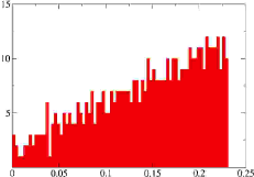
Figure 1: Histogram of the $512$ smallest eigenvalues of $\tilde{Q}^{2}(y,x)$.

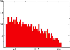
Figure 2: Histogram of the $512$ largest eigenvalues of $\tilde{Q}^{2}(y,x)$.

1 Tuning the Quadratically Optimized Polynomials

The quality of the approximation provided by the polynomial (66) does not only depend on its order, but also on the choice of the interval, where it should approximate the function under consideration. Now the optimal choice of the approximation interval, $[\epsilon,\lambda]$, will be determined for a quadratically optimized polynomial introduced in Sec. 1. Figure 3 displays the function

$$\lambda^{\alpha}P_{n_{1}}(\lambda)$$

of a quadratically optimized polynomial with $n_{1}=20$, $\alpha=1$ and $[\epsilon,\lambda]=[7.5\times 10^{-4},3]$. The quality of the approximation is best at the upper end of the interval, while already slightly above the upper limit it will soon become useless. At the lower end of the interval the approximation is worse, but the limit is not as stringent as in the former case.

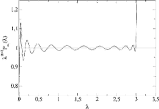
Figure 3: Test function $\lambda^{\alpha=1}P_{n_{1}=20}(\lambda)$ for a quadratically optimized polynomial.

These observations fix the strategy for finding the optimal interval: The upper limit must be chosen very conservatively — large enough that during the simulation runs an eigenvalue never leaves this interval. In the following, the choice $\lambda=3$ will be adopted unless otherwise stated. The lower end may be chosen more freely, in particular it may be chosen larger than the smallest eigenvalue since the eigenvalue density is largest in the middle of the interval. Raising the lower limit will make the approximation for the smallest eigenvalues worse, but will increase the quality of the polynomial in the middle, where the majority of eigenvalues is located.

Measures of Accuracy

To find a measure for the quality of the polynomial approximation for a particular matrix (in this case the square of the Hermitian Wilson matrix, $\tilde{Q}^{2}(y,x)$, for the gauge field configuration discussed above), the following two definitions of matrix norms will be adopted: Consider the matrix $R_{n}(\cdot)$ defined by

$$R_{n}(\tilde{Q}^{2})=\mathbf{1}-\tilde{Q}^{2\alpha}P_{n}(\tilde{Q}^{2})\,.$$ (1)

Then the following two definitions of matrix norms will be used:

1. Measure the vector norm of $|\xi(x)|$ defined by

   $$\xi(y)=\sum_{x}R_{n}(\tilde{Q}^{2})(y,x)\eta(x)\,,$$ (2)

   where $\eta(x)$ is a Gaussian random vector with unit width. The average vector norm $|\xi(x)|\equiv|\sum_{x}\xi(x)|$ for a sample of $\{\eta\}$ will be denoted by $|R_{n}(\tilde{Q}^{2})|$.

2. Measure the expectation value

   $$\langle R_{n}(\tilde{Q}^{2})\rangle=\sum_{\eta(x)}\sum_{xy}\eta^{\dagger}(y)R_{n}(\tilde{Q}^{2})(y,x)\eta(x)\,,$$ (3)

   where $\eta(x)$ is again a Gaussian random vector with width one. This quantity is not a norm, however. Since it is not positive definite the absolute value of $\langle R_{n}(\tilde{Q}^{2})\rangle$ will be used in the following and will be denoted by $\|R_{n}(\tilde{Q}^{2})\|$.

These definitions can also be applied to the case of the inverse square root defined in Eq. (76). This is done by replacing $R_{n}(\cdot)$ by $\hat{R}_{n_{3}}^{n_{2}}(\cdot)$, which is defined by

$$\hat{R}_{n_{3}}^{n_{2}}(\tilde{Q}^{2})=\mathbf{1}-\hat{P}_{n_{3}}(\tilde{Q}^{2})(\tilde{P}_{n_{2}}(\tilde{Q}^{2}))^{2}\,.$$ (4)

In particular, $\|\hat{R}_{n_{3}}^{n_{2}}(\tilde{Q}^{2})\|$ is the exponential factor in the noisy correction step of the TSMB algorithm, Eq. (78), if the old configuration is chosen equal to the new one.

When computing the matrix norms of $R_{n}$ for too small orders $n$, the fluctuations of the norms will be large. In particular, the matrix norm (3) at small $n$ will be close to (59), i.e. the inverse of the determinant of $\tilde{Q}$. The opposite limit $n\rightarrow\infty$ will correspond to the determinant itself. As has been discussed in Sec. 1, the fluctuations of (59) are huge, while those of its inverse are small. Thus, the fluctuations will decrease for increasing values of $n$. Therefore, the optimization of the static approximation should be performed for comparatively large orders.

Fixing the Lower Limit

As has been argued, it is of importance to have a recipe for fixing the lower limit of a quadratically optimized polynomial for a given order. First consider the choice $n_{1}=20$ for which the two matrix norms together with their standard errors are displayed in Fig. 4 for varying values of $\epsilon$. For each point a sample of $100$ Gaussian vectors has been considered. While $\|R_{20}\|$ displays a minimum at the lower end of the interval (where the smallest eigenvalue is located), $|R_{20}|$ stays more or less constant over a range of more than one order of magnitude. Thus, for small orders, one cannot rule out that a choice $\epsilon\gg\lambda_{\mbox{\tiny min}}$ is practical.

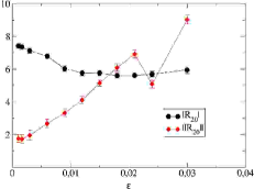
Figure 4: Norms $|R_{20}|$ and $\|R_{20}\|$ vs. the lower interval limit $\epsilon$.

Next consider the case $n_{1}=180$ which should already provide a very good approximation to the inverse function. Figure 5 again shows the two matrix norms for varying values of $\epsilon$. The curve of $|R_{180}|$ clearly displays a minimum at $\epsilon_{\mbox{\tiny opt}}=4.5\times 10^{-4}$, which is about $20\%$ smaller than $\lambda_{\mbox{\tiny min}}$. The curve of $\|R_{180}\|$ shows a more or less continuous increase with larger errors.

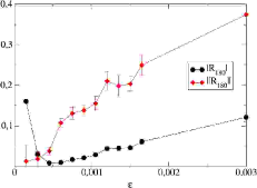
Figure 5: Norms $|R_{180}|$ and $\|R_{180}\|$ as defined in Eq. (2) vs. the lower interval limit $\epsilon$.

Finally the situation regarding the third polynomial must be clarified. In general, the systematic error of a simulation run should be bounded to be much smaller than the statistical error of any quantity measured. The magnitude of the error can be estimated by considering a noisy estimate for the determinant, Eq. (78), with the old configuration being equal to the new one, i.e.

$$U^{\prime}=U\,.$$

If the approximation was exact the acceptance probability would be equal to one. However, any deviation in the exponential could cause spurious acceptances or rejections. Since any negative value in the exponential in (78) would cause the configuration to be accepted in any case, the case of large negative values of the exponential factor can be completely disregarded. On the other hand, for large positive values of the argument, the influence of any error on the acceptance rate will be minor due to the flat tail of the exponential function. Thence, the largest influence is to be expected for values around zero.

To quantify the influence of this systematic error one can consider the following model for the exponential correction factor:

$$E(\sigma,b,x)=\frac{1}{\sqrt{2\pi}\sigma}\exp\left[-\frac{1}{2\sigma^{2}}\left(b-x\right)^{2}\right]\,.$$ (5)

The resulting acceptance rate can be computed to yield

$$P_{\mbox{\tiny acc}}(\sigma,b) = \int_{-\infty}^{0}dx\;E(\sigma,b,x)+\int_{0}^{\infty}dx\;E(\sigma,b,x)\exp(-x)$$ (6)

$$= \frac{1}{2}\left(1-\mbox{Erf}\left[\frac{b}{\sqrt{2}\sigma}\right]\right)+\frac{1}{2}\left(1-\mbox{Erf}\left[\frac{\sigma^{2}-b}{\sqrt{2}\sigma}\right]\right)\exp\left[-b+\frac{1}{2}\sigma^{2}\right]\,.$$

Using Eq. (6), one can compute the actual systematic error by measuring $\sigma$, $b$ and $\hat{R}^{n_{2}}_{n_{3}}(\tilde{Q}^{2})$ in a given run and considering the resulting change in acceptance rates

$$\Delta P_{\mbox{\tiny acc}}(\sigma,b,\Delta b=\|\hat{R}^{n_{2}}_{n_{3}}(\tilde{Q}^{2})\|)=|P_{\mbox{\tiny acc}}(\sigma,b)-P_{\mbox{\tiny acc}}(\sigma,b-\|\hat{R}^{n_{2}}_{n_{3}}(\tilde{Q}^{2})\|)|\,.$$ (7)

The resulting number is the systematic error for a single trajectory. As a rule of thumb one should not allow $\Delta P_{\mbox{\tiny acc}}(\sigma,b,\Delta b)$ to exceed values of $1\times 10^{-3}$. In most situations, however, it is possible to make it as small as $1\times 10^{-5}$. Any systematic error will then be negligible.

Figure 6 shows plots of the two norms with $n_{3}=200$ (the value $n_{2}=160$ has been chosen compatible to the situation discussed above) vs. the lower limit of the interval, $\epsilon$. Both norms obtain their minimal values at lower interval limits of $\epsilon\approx 7.5\times 10^{-4}\approx 1.5\times\lambda_{\mbox{\tiny min}}$. However, the important norm in this case is $\|\hat{R}_{n_{3}}(\tilde{Q}^{2})\|$ — already if $\epsilon$ is varied by a factor of $2$, one approaches a region where the systematic error may become significant. One has to keep in mind that in a dynamical simulation fluctuations may cause the smallest eigenvalue to become smaller than in the present case. Therefore, the interval for the third polynomial has to be chosen far more conservatively than for the other polynomials and the residual norm must be adjusted by increasing the order $n_{3}$.

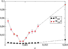
Figure 6: Residual norms for $\hat{R}^{160}_{200}(\tilde{Q}^{2})$ vs. the lower interval limit $\epsilon$.

In some cases, there is a different problem related to this strategy, cf. Sec. 3 below.

One can conclude that the choice of the approximation interval for quadratically optimized polynomials can have a large impact on the quality of the approximation. While in the case of the first polynomial (where one deals with a comparatively small order), the choice of the lower limit only has a small impact, the situation changes as the order is increased. For orders as large as the second polynomial in the two-step approximation, the optimal choice for the lower limit is slightly smaller than the smallest eigenvalue of the matrix, while for the third polynomial, the choice of the lower limit should be made extremely conservative. The interval should always cover every single eigenvalue and ensure that $\Delta P_{\mbox{\tiny acc}}$ in Eq. (7) is sufficiently small for the algorithm to be free of systematic errors.

In the case of a dynamical simulation, the choice of the interval should be guided by the average values of the smallest eigenvalue. However, this information is only rarely available prior to the run. It may therefore be necessary to readjust the polynomials during a run as more information becomes available. In this way one can reduce the total runtime, but at the price of more effort and logistics. Appendix 10 gives a framework for handling this type of runs.

In any case, one has to make sure that the third polynomial is sufficiently good by making a very conservative decision regarding the lower limit and making the order sufficiently large as to keep the systematic error bounded to at most a few percent.

2 Algorithm for Polynomials

As has been discussed in Sec. 3, different methods are possible for finding the polynomial, Eq. (66), which approximates the inverse of the Wilson matrix. The quadratically optimized polynomials do not require explicit knowledge of the eigenvalue density in the approximation interval. On the other hand, the method proposed by de Forcrand in [220] requires a thermalized gauge field configuration to be available. As has been noted in the latter publication, taking a single gauge field configuration may already be sufficient since the results from several configurations are similar.

Figure 3 already showed the deviation of a quadratically optimized polynomial. The GMRES algorithm discussed in Sec. 3 will now be used to construct the polynomial dynamically on a (different) thermalized configuration. The resulting plot of $\lambda^{\alpha=1}P_{n_{1}=20}(\lambda)$ is displayed in Fig. 7. For comparison the quadratically optimized polynomial from Fig. 3 is also shown.

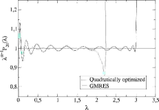
Figure 7: Polynomial $\lambda^{\alpha=1}P_{20}(\lambda)$ which has been obtained by applying the GMRES algorithm to a thermalized gauge field configuration together with the corresponding quadratically optimized polynomial.

It is apparent that the quadratically optimized polynomial performs worse in the middle of the spectrum, where most eigenvalues are located. In contrast, the GMRES polynomial respects the spectral density of the Wilson matrix and thus results in a better approximation. The disadvantage is that the underlying algorithm will become unstable when computing the coefficients of the polynomials for larger orders if it is only run on a machine with $64$-bit precision. This instability will already become apparent for orders slightly beyond $n_{1}=20$. A further problem is that usually one does not have a thermalized gauge field configuration for a particular physical point prior to the calculation. It is therefore necessary to perform the optimization process dynamically during the sampling and readjust the polynomials after a certain number of trajectories. Similar to the case of quadratically optimized polynomials, this requires more effort.

The influence of the qualitative difference is displayed in Fig. 8. The GMRES results are compared to the quadratically optimized polynomials for a number of different orders. The polynomial interval for the quadratically optimized polynomials has been chosen to be $[\epsilon,\lambda]=[6\times 10^{-4},2.5]$. The former choice clearly exhibits smaller residuals and is thus superior. However, since the computation has only been performed with $64$-bit precision, the numerical instabilities are already visible at $n_{1}=20$.

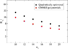
Figure 8: Residual vector norm for both the GMRES and the quadratically optimized polynomials.

This scheme can easily be extended to the case of any rational number $\alpha$, i.e. any rational number of fermion flavors. However, the instability of this method will also grow as the number of multiplications required increases. Therefore, this method has not been applied in the following. This is a place where further research is in demand. One way to solve this problem would be to implement the polynomial algorithm using very high precision arithmetics, similar to what has been done in [229]. Another way could consist of using a different scheme which does not recourse directly to the expansion coefficients in Krylov space.

3 Computing the Reweighting Correction

When using the TSMB algorithm for the correction step as discussed in Sec. 3, one will perform a noisy estimate for the inverse determinant using a static inversion algorithm with the polynomial $\tilde{P}_{n_{2}}(x)$. Any residual systematic error in the ensemble of gauge field configurations generated will then have to be repaired with a multicanonical reweighting. An observable will be computed using either (80) or (81).

In order to find an efficient way to perform this reweighting, it is assumed that the configuration under consideration has been computed using the TSMB algorithm with action (74), where the quadratically optimized polynomial (cf. Sec. 1) $P_{n_{1}}(x)\tilde{P}_{n_{2}}(x)\simeq P_{n_{1}+n_{2}=180}(x)$ has been employed with the interval $[\epsilon,\lambda]=[7.5\times 10^{-4},3]$. The overall systematic error from the simulation run is thus determined from the polynomial $P_{180}(x)$ alone. The observable under consideration is now $\hat{A}=1$, i.e. the correction alone is being measured. The correction factor from the individual $512$ lowest eigenvalues of $\tilde{Q}^{2}$ is plotted in Fig. 9. Obviously, the correction is mostly related to the lowest eigenvalue alone.

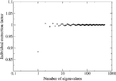
Figure 9: Individual correction factors as computed using the $512$ lowest eigenvalues of $\tilde{Q}^{2}(y,x)$ for the quadratically optimized polynomial $P_{180}(\tilde{Q}^{2})$.

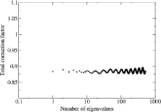
Figure 10: Similar to Fig. 9, but with the cumulative correction factor from the $512$ lowest eigenvalues.

This finding is confirmed when examining the convergence behavior of the correction factor with respect to the number of eigenvalues computed. The cumulative factor in Eq. (81) as a function of the number of eigenvalues taken into account is shown in Fig. 10 and gives an average value of $0.885$. Although larger eigenvalues still introduce fluctuations, the major impact comes from the smallest eigenvalue alone.

The alternative way to compute the correction factor is provided by the evaluation of (80). From $100$ noisy vectors one observes that the approximation already has converged at order $n_{4}=500$. The total correction factor from this method is

$$\langle 1\rangle_{P_{n_{4}=500}}=0.8783\pm 0.0113\,,$$

which is completely consistent with the value obtained from Fig. 10.

In conclusion, when estimating the correction factor on the basis of eigenvectors on an $\Omega=8^{4}$ lattice alone, it makes sense to use only a small fraction (definitely less than $32$) of the lowest eigenvalues. The fluctuations introduced from the larger eigenvalues do not have a significant influence on the total result. The evaluation of the correction factor using a fourth polynomial is a practical alternative and avoids having to compute a fraction of all eigenvalues. The only potential problem is that the smallest eigenvalue of $\tilde{Q}^{2}(y,x)$ may lie outside the interval of $P_{n_{4}}(\cdot)$, which could result in incorrect results. This problem can again be controlled by choosing an extremely conservative lower limit $\epsilon$ or even $\epsilon=0$. Once one considers larger lattices up to $\Omega=32\times 16^{3}$ and beyond, the eigenvalue approach may become too costly since the eigenvalue density increases linearly with the volume and consequently a larger number of eigenvalues need to be computed to cover an equivalent fraction of the spectrum.

2 Tuning the Dynamical Parameters

After the optimal matrix inversion using a non-adaptive polynomial for a single (or a limited set of) gauge field configurations has been found, there remains the task to examine the dynamical behavior of these approximations. This is a question of major interest for the practical implementation of any multiboson algorithm, since after all one is interested in using the approximations in a dynamical updating process. It may happen, that fluctuations of the eigenvalue density may temporarily cause eigenvalues to run out of the approximation interval. This can have a dramatic impact on the performance of the algorithm. It is therefore of considerable importance to assess the size of these fluctuations and what impact they could have on a simulation run. It is important to notice that these aspects may still be explored on rather small lattices since they will exhibit larger fluctuations and will thence show a larger sensitivity to these vulnerabilities.

1 Practical Determination of Autocorrelations

Before proceeding further, the tools must be prepared to compute the primary measure of efficiency in the dynamical case, namely the autocorrelation time of a time series. Since the aim of any simulation algorithm is to generate statistically independent gauge field configurations with minimal effort, the autocorrelation time is the key monitor for the cost determination of a particular algorithm. The theoretical bases of methods to compute autocorrelations of time series have been laid in Sec. 2. The purpose of this section is to apply them to two different time series obtained from actual simulation runs.

In the first case, the series has a low fluctuation and is sufficiently long for the autocorrelation time to be measured. The second situation is less suitable: the time series exhibits large fluctuations and a rather large autocorrelation time. Furthermore, it shows a contamination of a very long mode which introduces fluctuations on a time scale comparable to the length of the series itself. This mode appears to be separated from the other modes contained in the series. Given the fact that the total lattice size is given by $L\approx 1.128$ fm (cf. Tab. 1), one may suspect that the simulation is already very close to the shielding transition, see also Sec. 1. This could explain the observed behavior and the presence of the long-ranged mode. This mode contaminates the results and unless it is possible to perform simulations on a series at least two orders of magnitude longer, no statement can be made about its length. In this case it will become evident, that the lag-differencing method as discussed in Sec. 5 is still able to extract information from the series although the other methods fail.

Case I: Low Fluctuations

This time series has been taken from a simulation run using the physical parameters displayed in Tab. 1 on an $\Omega=32\times 16^{3}$-lattice. The algorithm employed is the HMC algorithm with SSOR-preconditioning. The molecular dynamics integration algorithm is the leap-frog scheme with a time step of $\Delta t=1\times 10^{-2}$ and a trajectory length of $n_{\mbox{\tiny MD}}=100\pm 20$. The resulting acceptance rate is $71.6\%$.

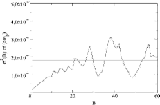
Figure 11: Jackknife variances for different bin sizes for the mass of the vector meson with three dynamical fermions at $\beta=5.2$ and $\kappa=0.156$. The mass is obtained from a fit to an interval $[t_{\mbox{\tiny min}}=5,t_{\mbox{\tiny max}}=7]$.

The total size of the sample consists of $4518$ trajectories, from which the leading $1000$ trajectories have been discarded. The complete time series is given in Fig. 11.

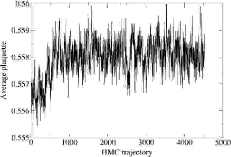
Figure 11: Plaquette history of HMC run.

Figure 12 shows the normalized autocorrelation function (dotted curve), together with the integrated autocorrelation time (blue curve) as a function of the cutoff. The windowing procedure discussed in Sec. 5 has been applied with $c=4,6$ resulting in the green and red lines, respectively. From the $c=6$ line, one can read off an integrated autocorrelation time of $\tau_{\mbox{\tiny int}}=11.28\pm 0.43$. The dashed-dotted line displays the maximum of the curve, which is clearly compatible with the $c=6$ window.

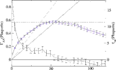
Figure 12: Normalized autocorrelation function and integrated autocorrelation time vs. the cutoff for the HMC plaquette history.

A particular problem is already visible in the behavior of the normalized autocorrelation function. It does not approach zero exponentially (as one would expect), but appears to reach a plateau above zero, before it suddenly drops. The curve is not compatible with zero at this point since it is almost two standard deviations too high. This is a typical case of a linear bias mentioned in Sec. 5. The lag-differencing method which will be applied below is able to handle this situation.

Next, the variance is estimated using the Jackknife method (cf. Sec. 5). Figure 13 shows the variance $\sigma_{B}(\mbox{Plaquette})$ as a function of the bin size $B$. The variance reaches a plateau (red line) at $\sigma(\mbox{Plaquette})\approx(1.41\pm 0.53)\times 10^{-9}$ which yields the true variance of the plaquette. The result for $B=1$ is given by $\sigma_{B=1}(\mbox{Plaquette})=7.53\times 10^{-11}$. Applying Eq. (30) now yields $\tau_{\mbox{\tiny int}}\approx 9.36\pm 3.52$, which is slightly below the result from the previous methods, but with a much larger uncertainty. It must be realized that this procedure should only give a rough estimate of the “true” value of $\tau_{\mbox{\tiny int}}$, see [148] for a thorough discussion.

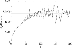
Figure 13: Variance $\sigma_{B}(\mbox{Plaquette})$ vs. the bin size $B$ using the Jackknife method for the HMC plaquette history.

Finally the lag-differencing method (cf. Sec. 5) is applied to the time series. As a first step, the order-$1$-lag-$30$-differenced series, $D_{l=30}^{(k=1)}(\mbox{Plaquette})$, is computed using the definition (5). It is displayed in Fig. 14. As the next step, the correlation between the plaquette and $D_{30}^{(1)}$ is being computed, cf. (27). The normalized correlation function, $\Gamma_{A,(D_{30}^{(1)}A)}(t)$, together with its integral as a function of the cut-off is shown in Fig. 15. The former is given by the dotted curve, while the latter is visualized by the blue line. The windowing method proposes the values $\tau_{\mbox{\tiny int}}=5.94\pm 0.34$ (green line) and $\tau_{\mbox{\tiny int}}=10.26\pm 0.55$ (red line) for windows of $c=4$ and $c=6$, respectively. The maximum of the autocorrelation function, however, is reached at $\tau_{\mbox{\tiny int}}=12.11\pm 0.48$. It is obvious that there is no significant improvement from the differencing prescription and that the resulting function $\Gamma_{A,(D_{30}^{(1)}A)}(t)$ is not compatible with a single exponential mode, just like the original function $\Gamma_{AA}(t)$ was not. Furthermore, the maximum of the curve has shifted to the left and the windowing prescription does no longer give the maximum at $c=6$. In fact, the differencing prescription impairs the statistics if the lag is large compared to the “true” autocorrelation time.

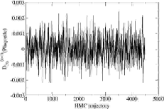
Figure 14: Order-$1$-lag-$30$ differenced series of the HMC plaquette history.

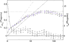
Figure 15: Correlation function $\Gamma_{AD_{30}^{(1)}A)}(t)$ together with its integral vs. the cutoff.

To obtain a better result from the lag-differencing method, one has to repeat the procedure leading to the estimate for $\tau_{\mbox{\tiny int}}$ using a series of different lags and look for the stability of results. As long as the lag $l$ stays above the autocorrelation time, no physical modes should get lost. Once the autocorrelation time obtained becomes as large as or larger than the lag $l$, one may cut off physical modes. Thus — in accordance with the discussion in Sec. 5 — one would look for a plateau at some intermediate values of $l$, where the autocorrelation function should exhibit an exponential behavior.

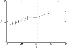
Figure 16: Integrated autocorrelation time as obtained from the lag-differencing method for varying lags $l$.

The results from this analysis are displayed graphically in Fig. 16. Indeed, one finds a plateau reaching from $l\approx 22$ up to $l\approx 26$ giving rise to $\tau_{\mbox{\tiny int}}=10.96\pm 0.39$. The self-consistency criterion $\tau_{\mbox{\tiny int}}>l$ is clearly met. The question arises, whether the differencing prescription does indeed result in a correlation function where the linear bias is suppressed. To address this question, Fig. 17 shows the correlation function for the case $l=23$. Now the function indeed decays to zero for already a short value of the cutoff, but still increases later on. This may be no exponential mode, but a polynomial mode giving rise to a higher order bias. Although in theory one could get rid of this bias by considering a higher-order differencing scheme, the impact of this procedure on the quality of statistics would invalidate this approach pretty soon. In particular, if the quality of the series was good enough to allow for higher-order differencing, the impact of the bias would be significantly smaller in the first place.

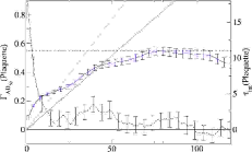
Figure 17: Similar to Fig. 15, but with a differencing lag $l=23$.

The lesson from this investigation is that the linear bias can be removed by applying the lag-differencing prescription and the result obtained in this way is consistent with the one obtained from the original autocorrelation function and from the Jackknife method. The analysis shows that for the HMC with dynamical fermions one has to use a time series with a length of at least $4000$ trajectories to gain accurate information about the true autocorrelation behavior.

Case II: Large Fluctuations

The second series has been obtained from the history of the average plaquettes using the TSMB algorithm discussed in Sec. 3. The simulation has been performed using the same physical parameters as in the previous case except for the volume and the algorithmic parameters given in Tab. 3. The first polynomial order was $n_{1}=20$. This run is part of the tuning series discussed in Sec. 2 below. Reweighting of the observables has been neglected, since this would have introduced another source of autocorrelation effects, see [230] for a discussion. The total length of the series was $51196$ trajectories, where the thermalization phase has already been subtracted.

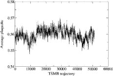
Figure 18: Time series of the average plaquette from the TSMB algorithm.

As has already been pointed out, a very long mode possibly related to the shielding transition is present in the series which cannot be examined in a time series of such a length. However, since this mode does not appear to have any connection to the other, short-range fluctuations, it may be questioned if it has any significance for the efficiency considerations of the multiboson algorithms.

As in the previous case, first the autocorrelation function is visualized together with the corresponding integral in Fig. 19. The estimated autocorrelation time is $\tau_{\mbox{\tiny int}}=1897\pm 135$. Again, the problem is that the autocorrelation function does not go to zero exponentially and that it appears to reach a plateau, before it drops to zero and then decreases linearly. This behavior may indicate a linear bias, which could be removed by the lag-differencing method.

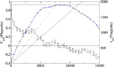
Figure 19: Autocorrelation function and the corresponding integral as a function of the cutoff for the plaquette history from the TSMB run.

The variance obtained from the Jackknife analysis for different bin sizes is shown in Figure 20. The plateau can be estimated to lie at about $\sigma(\mbox{Plaquette})\approx(5.855\pm 2.422)\times 10^{-7}$. Together with $\sigma_{B=1}(\mbox{Plaquette})=2.032\times 10^{-10}$ one obtains an estimate of $\tau_{\mbox{\tiny int}}\approx 1441\pm 596$. This number is compatible with the previous estimate, however it should not be trusted since the original time series was contaminated with the mode too long to be reliably examined.

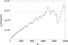
Figure 20: Jackknife variance calculated for different bin sizes for the time series from the TSMB run.

Finally, the lag-differencing method has to shed some light on the behavior of the autocorrelation time. Figure 21 displays the results from measuring the integrated autocorrelation time with various lags. If the long-range mode is indeed separated from the other modes, one should be able to see a plateau from the other modes after the long-range mode has been cut out. There is a clear signal for the formation of such a plateau at lags between $l=600$ and $l=800$. Using the error bars from the single points and making a linear fit yields $\tau_{\mbox{\tiny int}}=334.3\pm 65.6$. This result is about a factor of four below the previous estimates.

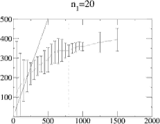
Figure 21: Integrated autocorrelation time vs. the differencing lag for the TSMB run.

In conclusion, the lag-differencing method allows to get rid of a linear bias and thus enables the evaluation of a series with large fluctuations. The stability criterion is met, i.e. the estimated autocorrelation time exhibits a plateau when plotted as a function of the lag $l$. The self-consistency criterion is also met, i.e. the resulting value for $\tau_{\mbox{\tiny int}}$ is larger than the current value of $l$ used. A large autocorrelation mode associated with a fluctuation that is expected to vanish with increasing volume, has successfully been cut off. In the following section, a series of these runs will be presented, which are all identical except that a single parameter has been changed during all runs.

2 Acceptance Rates vs. Polynomial Approximation Quality

It has already been argued that the number of boson fields enters linearly into the autocorrelation time of a multiboson algorithm. On the other hand, one can expect that a small number of boson fields gives rise to a small acceptance rate and thence to an increase in the autocorrelation time again for small numbers of fields. The number of boson fields and thus the first polynomial order is of critical importance for a multiboson algorithm. Until today, however, no systematic analysis of this effect has been performed and the impact of this choice on practical simulations is unclear. This is certainly related to the fact that any systematic analysis is exacerbated by the requirement to measure autocorrelation times with a reasonable accuracy. Therefore, we base our study on very long runs. Beyond that, we employ the efficient tools described in detail in the previous section.

The algorithmic parameters shared by all runs are displayed in Tab. 3. Only the order of the first polynomial, $n_{1}$, has been varied.

$\mathbf{n_{1}}$	$\mathbf{n_{2}}$	$\mathbf{n_{3}}$	$\mathbf{[\epsilon,\lambda]}$	Updates/Trajectory
var.	$160$	$200$	$[7.5\times 10^{-4},3]$	$1$ boson HB, $3$ boson OR, $2$ gauge Metropolis, $1$ noisy corr.
Volume $\Omega=8^{4}$

Table 3: General algorithmic parameters for high-statistics TSMB runs.

Table 4 shows the statistics generated together with the acceptance rates of the noisy correction step and the cost of a single trajectory. These runs have been performed on the ALiCE computer cluster installed at Wuppertal University. The machine configurations were both a single node configuration (with no parallelization) and a four-node partition with the lattice parallelized in $z$- and $t$-direction. The local lattice size was consequently $\Omega_{\mbox{\tiny loc}}=4\times 8\times 8\times 4$. The numerical efforts are given for the latter situation.

$n_{1}$	Number of confs.	Acceptance rates	Numerical effort/MV-Mults
$12$	$101111$	$8.00\%$	$463.0$
$18$	$62462$	$39.61\%$	$499.6$
$20$	$61196$	$51.51\%$	$511.8$
$22$	$42248$	$57.94\%$	$524.0$
$24$	$49704$	$64.56\%$	$536.2$
$26$	$50684$	$69.45\%$	$548.4$
$28$	$50412$	$74.46\%$	$560.6$
$32$	$50238$	$80.84\%$	$585.0$

Table 4: Runs for the parameter tuning of the TSMB algorithm.

It is specified in terms of a multiplication by the preconditioned fermion matrix $\tilde{Q}^{2}(y,x)$ with an arbitrary colorspinor $\eta(x)$. Since the TSMB algorithm uses non-adaptive polynomials in the noisy correction step, the number of explicit matrix-vector multiplications is straightforwardly given by $n_{2}+n_{3}$. In the case under consideration we thus have $n_{2}+n_{3}=360$. To estimate the total effort we assume that the efficiency of the implementation for the local algorithms is roughly equivalent to the efficiency of the matrix-vector multiplication routine. Thencefrom, we measure the time needed for a complete trajectory, $t_{\mbox{\tiny traj}}$, and the time needed for the noisy correction alone, $t_{\mbox{\tiny noisy}}$. Using these times, we can define the total effort $E_{\mbox{\tiny MV-mults}}$ as

$$E_{\mbox{\tiny MV-mults}}=\left(n_{2}+n_{3}\right)\frac{t_{\mbox{\tiny traj}}}{t_{\mbox{\tiny noisy}}}\,.$$ (8)

Behavior of the Correction Factor

As a first step, the dependence of the acceptance rate on the magnitude of the exponential correction factor $\exp\left(-C_{12}\{U_{\mbox{\tiny old}},U_{\mbox{\tiny new}}\}\right)$ should be clarified. Figure 22 shows the exponential correction factor together with its standard deviation. It depends exponentially on the order $n_{1}$.

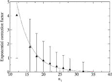
Figure 22: Dependence of the exponential correction factor on the number of boson fields, $n_{1}$.

The function approximating the average value is given by

$$\left[\exp\left(-C_{12}\right)\right]\left(n_{1}\right) = A\cdot\exp\left(-B\cdot n_{1}\right)\,,$$ (9)

$$A=78.657\,,\;B=0.23092\,.$$

This behavior is in line with the expectations that the convergence of the first polynomial is exponential. On the other hand, the standard deviation of the exponential correction does not follow a precise exponential dependence; this is shown in Fig. 23.

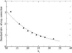
Figure 23: Dependence of the standard deviation of the exponential correction factor on the number of boson fields, $n_{1}$.

Restricted to the intermediate regime, nevertheless an exponential function yields a good fit to the data points:

$$\langle\left[\exp\left(-C_{12}\right)\right]\rangle\left(n_{1}\right) = A^{\prime}\cdot\exp\left(-B^{\prime}\cdot n_{1}\right)\,,$$ (10)

$$A^{\prime}=6.6765\,,\;B^{\prime}=0.075757\,.$$

Finally, inserting the models (9) and (10) into Eq. (6) allows to check their validity by comparing them to the measured acceptance rates from Tab. 4. Table 5 compares the predicted and the measured acceptance rates. The numbers are obviously in perfect agreement.

$\mathbf{n_{1}}$	Model	Measured
$12$	$8.64\%$	$8.00\%$
$18$	$43.84\%$	$39.61\%$
$20$	$53.34\%$	$51.51\%$
$22$	$60.88\%$	$57.94\%$
$24$	$66.84\%$	$64.56\%$
$26$	$71.59\%$	$69.45\%$
$28$	$75.45\%$	$74.46\%$
$32$	$81.37\%$	$80.84\%$

Table 5: Comparison of acceptance rates as a function of $n_{1}$ from the predictions of Eq. (6) and from the actuals runs in Tab. 4.

In conclusion, the exponential correction factor shows an exponential dependence on the order $n_{1}$. Its standard deviation also approximately follows an exponential decay. Therefore, the acceptance rate can be predicted as a function of the polynomial order $n_{1}$ once at least two points have been determined which allow to fit the functions (9) and (10).

Fermionic Energy

First consider the fermionic action $S_{\mbox{\tiny f}}$. This quantity is not affected by the correction step, since in the trajectory in Tab. 3 the correction step may only reject an update of the gauge field. However, it is still linked to the full dynamics of the system by its coupling to the gauge field. Thus, it is expected to display a linear dependence on the number of boson fields, $n_{1}$. Figure 24 shows the integrated autocorrelation times $\tau_{\mbox{\tiny int}}\left(S_{\mbox{\tiny f}}\right)$ versus the polynomial order, $n_{1}$. The autocorrelation times have been measured using the windowing prescription from Sec. 5 on the integrated autocorrelation function.

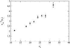
Figure 24: Integrated autocorrelation time $\tau_{\mbox{\tiny int}}\left(S_{\mbox{\tiny f}}\right)$ vs. the number of boson fields $n_{1}$.

One finds a linear dependence on the number of boson fields. Certainly, the small absolute values of the fermionic autocorrelation times help to make the measurement very precise. However, the fermionic energy does not directly give rise to any useful physical information. Rather quantities computed directly from the gauge fields (like the plaquette) give rise to physical information about the system. Since the “fermionic force” on the gauge field is directly related to the boson fields, one can nonetheless expect the influence on the autocorrelation time of gauge-field related quantities to be linear in $n_{1}$. Unfortunately, the situation is far more involved in that case.

Gauge Field Plaquette

Since the plaquette is a purely gauge-field dependent quantity, its autocorrelation time will be affected by the acceptance rate. It can be expected to increase at too small $n_{1}$ because of the correlations caused by identical configurations. Furthermore, as already noted above, the plaquette contains a strong noise and is thus very difficult to be measured. The desired behavior will therefore be embedded in huge fluctuations. A standard analysis of the effect is therefore bound to fail. It is in this situation, where the lag-differencing method becomes important and provides a useful source of information.

The integrated autocorrelation time as a function of the differencing lag is shown in Fig. 25 for all available values of $n_{1}$. The errors are larger than in the case of $S_{\mbox{\tiny f}}$ since the autocorrelation times are now larger and thus the statistics for this observable is worse. The left diagram in the second row has already been discussed in Sec. 1, Fig. 21.

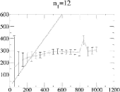
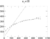
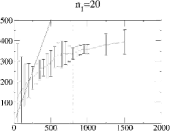
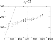
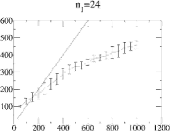
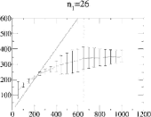
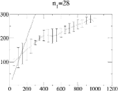
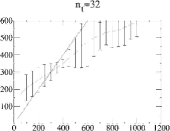
Figure 25: Integrated autocorrelation times of the plaquette together with their standard errors as a function of the differencing lag for various $n_{1}$.

In the case $n_{1}=12$ a plateau is clearly visible, indicating that the lag-differencing yields a stable solution. In the case $n_{1}=18$ the situation is less clear. A pseudo-plateau may be suspected around $l=600$, but in general the method is unstable and the result should be disregarded. The case $n_{1}=20$ has been discussed in Sec. 1, while $n_{1}=22$ is again very stable with a plateau determined around $l=600$. Absolutely nothing can be learned from $n_{1}=24$; there is no plateau and obviously any attempt to find one is futile. For $n_{1}=26$ a clear plateau is again visible, starting at about $l=650$. Regarding $n_{1}=28$ a plateau can be found from $l=400$ to $l=600$. For $n_{1}=32$, again no result can be found.

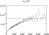
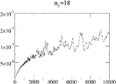
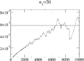
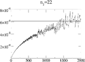
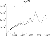
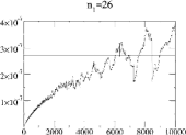
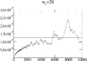
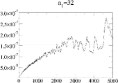
Figure 26: Jackknife variances as a function of the bin size for various values of $n_{1}$.

For comparison the Jackknife procedure as discussed in Sec. 5 has been applied to all samples. The variances vs. the bin sizes are displayed in Fig. 26. The straight lines give the plateau values. Again, the first graph in the second row is identical to Fig. 20 in Sec. 1.

The resulting integrated autocorrelation times read off from Figs. 25 and 26 are given in Tab. 6. Figure 27 displays these results graphically.

The conclusion is that there is no measurable increase in the autocorrelation time as $n_{1}$ is increased if one relies solely on the lag-differencing method. The increased acceptance rate from larger $n_{1}$ compensates for the loss of mobility in phase space. From this point of view it appears reasonable to simulate at comparatively small acceptance rates.

The Jackknife method exhibits a similar behavior, but it is compatible with a decrease of the autocorrelation time with increasing $n_{1}$. There is no indication, however, that this decrease exceeds a factor of two, see the cases $n_{1}=12$ and $n_{1}=32$. In fact, it is very likely that there is a non-trivial dependence (which results in differences of the order of a factor of two, but not much larger) which will become visible if one performs the same runs with far larger statistics. This is impossible with current computer technology, and would not be worth the effort given the fact that its influence is so small. The conclusion is therefore unchanged.

$n_{1}$	$\tau_{\mbox{\tiny int}}$ from LDM	Lag $l$	$\tau_{\mbox{\tiny int}}$ from Jackknife
$12$	$288.0\pm 20.5$	$400-800$	$885\pm 679$
$18$	$320.1$ (?)	$600$ (?)	-
$20$	$334.3\pm 65.6$	$600-800$	$1441\pm 596$
$22$	$174.3\pm 15.3$	$600-700$	$203\pm 54$
$24$	-	-	$680\pm 333$
$26$	$344.3\pm 73.7$	$650-1000$	$779\pm 335$
$28$	$212.9\pm 29.6$	$400-600$	$409\pm 390$
$32$	-	-	$386\pm 89$

Table 6: Integrated autocorrelation times of the plaquette together with their standard errors as read off from Fig. 25.

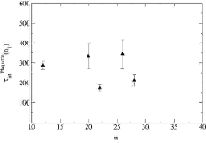
Figure 27: Integrated autocorrelation times of the plaquette vs. $n_{1}$.

3 Dynamical Reweighting Factor

Of particular importance is the stability of the polynomial approximation with respect to the interval $\left[\epsilon,\lambda\right]$ chosen for the TSMB algorithm. To access this problem, three runs have been performed with different choices for the lowest limit $\epsilon$. The physical parameters were again chosen according to Tab. 1 on an $\Omega=8^{4}$ lattice using the TSMB algorithm with polynomial order $n_{1}=20$ and parameters as in Tab. 3 apart from the value of $\epsilon$. The lower limit has been varied to be $\epsilon=4.5\times 10^{-4}$ in the first, $\epsilon=6.0\times 10^{-4}$ in the second, and $\epsilon=7.5\times 10^{-4}$ in the final case. These polynomials are visualized in Fig. 28 for the lower end of the approximation intervals.

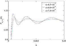
Figure 28: Polynomials $P_{n_{1}}(\lambda)\cdot P_{n_{2}}(\lambda)\simeq P_{n_{1}+n_{2}}(\lambda)$ for the three different values of the lower limit.

The histories of the reweighting factors measured during the runs are displayed in Fig. 29. They have been computed from the lowest $32$ eigenvalues (cf. Sec. 3).

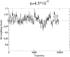
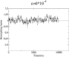
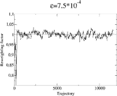
Figure 29: Reweighting factors for the three values of $\epsilon$.

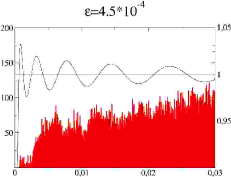
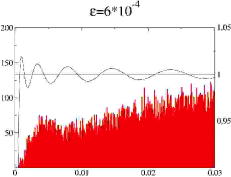
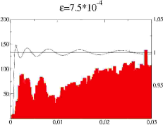
Figure 30: Accumulated eigenvalue histograms for the $32$ lowest eigenvalues of $\tilde{Q}^{2}$ for the three runs.

In the first case, $\epsilon_{1}=4.5\times 10^{-4}$, the correction factor shows the largest fluctuation of all cases: $\Delta_{1}=1.006990\pm 0.028267$. For the second case, $\epsilon_{2}=6.0\times 10^{-4}$, one obtains a correction factor of $\Delta_{2}=1.005144\pm 0.016978$. In the third case with $\epsilon_{3}=7.5\times 10^{-4}$ the correction factor drops down to $0.75$ meaning that the lowest eigenvalue left the region where the polynomial approximation is good enough; although this appears to be a problem, it only happens at a single place and never repeats. If this outlier is not disregarded, the correction factor is found to be $\Delta_{3}=0.997461\pm 0.021883$. Dropping the first $500$ trajectories from the sample — which is certainly justified, since it makes up only $5\%$ of the total runtime — one arrives at $\Delta_{3}=0.999619\pm 0.012296$. When computing any observable, however, the configurations must not be disregarded, since the algorithm would otherwise not be ergodic. If it is included in the measurement via Eq. (80), the algorithm will be both exact and ergodic.

As it is apparent from Fig. 28 (see also Fig. 3), the correction factor oscillates for the contributions from the smallest eigenvalues when using the static inversion of the TSMB algorithm. Consequently, an eigenvalue which is located in a “valley” will contribute with a smaller factor than an eigenvalue located on a local maximum. The static inversion of the TSMB algorithm may prefer to accumulate the eigenvalues in the local minima compared to the distribution sampled by an adaptive inverter. Since the distributions from the adaptive inversion (or from the reweighted static inversion, respectively) do not know about the existence of the oscillations, one may suspect that this distortion of phase space introduces notable stochastic forces. If these forces were present, they could result in larger autocorrelation times since motion of the eigenvalues between separate valleys would be suppressed. Figure 30 shows the histograms of the $32$ lowest eigenvalues from the three histories of the runs, computed every $100$ trajectories.

There does not appear to be any correlation between the eigenvalue fluctuations and the shape of the polynomials. As a result, one can say that the static matrix inversion employed in the TSMB algorithm does not result in significant stochastic forces. Furthermore, it is possible to make a choice of $\epsilon$ guided by the optimal lower limits found in Sec. 1. If the lowest eigenvalue ever leaves this interval, the correction factor will suppress these configurations. On the average, it will be smaller (with all other parameters fixed) than any choice with smaller $\epsilon$. The magnitude of the reweighting factor is then controlled by the choice of $n_{2}$. Since a large fluctuation of the reweighting factor impairs the statistics, the value of $n_{2}$ should be chosen such that the reweighting factor is always below the statistical error. This choice ensures that its influence is so small that the statistical quality of the sample is not perturbed too much. Alternatively, one can also compute the determinant norm $\|R(\tilde{Q}^{2})\|$ given by Eq. (3) for the second polynomial and keep its error below the statistical one. The latter procedure is simpler and still gives a good handle of the quality attained.

On the other hand, one should refrain from making $n_{2}$ far too large and the lower limit $\epsilon$ too small — this choice will simply increase the computer time required and make the algorithm inefficient.

4 Updating Strategy

After the recipe for choosing the polynomials and their orders are fixed, finally the focus is placed on the tuning of the updating algorithms for sampling a new configuration (the transition matrix ${\cal P}$ in the Markov process). The available algorithms have all been discussed in detail in Sec. 4.

Boson Field Updates

The boson field updates should be performed using a global heatbath (cf. Sec. 2) to achieve optimal decorrelation. This fact is already known theoretically from [196] and has been confirmed numerically in [221]. The global updates may, however, be accompanied by local updates, see e.g. [197].

Prior to a simulation run, the boson fields should be thermalized. This can best be achieved by holding the gauge field configuration fixed and updating the boson fields only. Observing the efficiency of thermalization methods also allows to shed some light on the best combination of local updating algorithms. Figure 31 shows a history of the fermionic energy, $S_{\mbox{\tiny f}}$, starting from a random boson field configuration. They display the effect of local overrelaxation sweeps to the thermalization. The runs have been performed using an $\Omega=4^{4}$ lattice. The physical parameters have been chosen as in Tab. 1 and the polynomial order has been chosen to be $n_{1}=60$. This makes no sense for a production run on this lattice size, but since the local boson field updates factorize, there should be no dependence on the number $n_{1}$ chosen. The interval of the polynomial has been chosen to be $[\epsilon,\lambda]=[7.5\times 10^{-4},3]$. A trajectory always consisted of a local boson heatbath update and either $0$, $1$ or $3$ local boson field overrelaxations. It is obvious, that local boson overrelaxations improve the thermalization rate and thus should also be expected to decrease the exponential autocorrelation time.

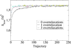
Figure 31: Boson field thermalization using local boson field updating algorithms.

Of course, in practical implementations, one should not use the local updating algorithms for the thermalization, but instead directly use the global boson heatbath.

Gauge Field Updates

For the gauge field updates one can either use a local Metropolis algorithm (Sec. 1), a local heatbath (see Sec. 2), or local overrelaxations (Sec. 3). It turns out that after a certain number of gauge field updates has been applied the acceptance rate of the noisy correction step stays essentially constant.

To demonstrate this behavior, a simulation run at the physical parameters given in Tab. 7 on a lattice with $\Omega=8^{4}$ has been performed. This run is a part of the investigations performed in Sec. 1. Table 8 shows the algorithmic parameters in this study. The only parameter varied is the number of gauge field Metropolis sweeps, where a Metropolis algorithm with eight hits per single link has been used.

$\mathbf{N_{f}^{\mbox{\tiny{sea}}}}$	$\mathbf{\beta}$	$\mathbf{\kappa}$
$3$	$5.3$	$0.150$

Table 7: Physical parameters for the investigation of the gauge field updating sequence.

$\mathbf{n_{1}}$	$\mathbf{n_{2}}$	$\mathbf{n_{3}}$	$\mathbf{\left[\epsilon,\lambda\right]}$	Updates/Trajectory
$24$	$100$	$140$	$[1\times 10^{-2},3]$	$2$ boson HB, $6$ boson OR, var. gauge Metropolis, $1$ noisy corr.
Volume: $\Omega=8^{4}$

Table 8: Algorithmic parameters for the investigation of the gauge field updating sequence.

The resulting values of the exponential correction together with their standard deviations and the corresponding acceptance rates are shown in Tab. 9.

Metropolis sweeps	$\mathbf{\exp(-C_{12})}$	Std. dev. of $\mathbf{\exp(-C_{12})}$	Acceptance rate
$2$	$0.663$	$1.125$	$59\%$
$4$	$1.000$	$1.421$	$48\%$
$6$	$1.350$	$1.371$	$41\%$
$8$	$1.188$	$1.523$	$52\%$
$12$	$1.120$	$1.429$	$48\%$

Table 9: Exponential correction with standard deviation and the corresponding acceptance rates as a function of the number of gauge field Metropolis sweeps.

The average exponential correction increases slightly with an increasing number of sweeps between the noisy corrections. However, this increase is accompanied by a slight increase in the standard deviation. Already after six sweeps have been performed, the changes can be attributed to fluctuations. The net effect is that the acceptance rate does not vary more than $10\%$. Hence, one finds that indeed the acceptance rate will saturate once a certain amount of updates has been applied to the gauge field.

Therefore it is possible to choose a rather large number of gauge field updates between the noisy corrections.

Choice of Updating Sequence

During a single trajectory, all d.o.f. of the system need to be updated. Therefore, a trajectory always consists of a certain number of boson field updates and a certain number of gauge field updates followed by a noisy correction step. The optimal sequence, however, might also depend on the architecture used for the configuration sampling. The reason is that the ratio of local to global update sweeps itself depends on the architecture used, see Sec. 3 below for details.

The acceptance rate is only slightly influenced by the number of local gauge field sweeps, as has been shown in Sec. 2. Hence, it is obvious that the noisy correction does not contribute to any reduction of the autocorrelation time while the update sweeps do. Consequently, one should always keep the number of local updates in a trajectory as large as possible, such as to minimize the contribution of the noisy correction step to the total runtime.

Now two different kinds of trajectories are proposed:

• Perform a number of boson field updates, followed by a number of gauge field updates and a correction step.

• Perform an alternating sequence of gauge and boson field updates prior to a correction step.

Since the correction step only depends on the gauge field configuration, but not on the boson fields, a rejection in the first proposal does not imply the necessity of restoring the boson field configuration since it has always been obtained in the background of a “valid” gauge field “background” configuration. Conversely, the second scheme will have to restore both the old boson and gauge field configurations in case the update is rejected. Hence, the memory requirements of the second proposal will be significantly larger than in the first case.

These considerations do not yet fix the optimal mixture of gauge and boson field updates. A very simple proposal is to use a single local gauge overrelaxation sweep followed by a single local boson overrelaxation sweep. The overrelaxation sweeps allow for a very fast movement through phase space, but do not ensure ergodicity, see Sec. 3. So this sequence has to be complemented by at least one ergodic heatbath and/or Metropolis sweep. This simple sequence turns out to be quite efficient in practice, see Sec. 2 for an application.

However, given the fact that the fermionic energy decorrelates much faster than the gauge field plaquette (see Sec. 2 above), one might hope that subsequent updates of the gauge field alone might still decrease the plaquette autocorrelation, although essentially only a small subset of all d.o.f. is being updated. The reason why this could be efficient is, as will be shown below in Sec. 4, that the caching of the boson field contributions as proposed in App. 9 in Eqs. (37) and (2) allows for a larger number of subsequent gauge-field-only update sweeps. On the other hand it is clear that this effect will very soon lead to a saturation since the gauge field will thermalize with the fixed boson field background.

The question when this saturation occurs can only be answered in a practical simulation. The physical parameters have again been chosen from Tab. 1, and the algorithmic parameters are given in Tab. 10. They are identical to the parameters given in Tab. 3.

$\mathbf{n_{1}}$	$\mathbf{n_{2}}$	$\mathbf{n_{3}}$	$\mathbf{[\epsilon,\lambda]}$
$20$	$160$	$200$	$[7.5\times 10^{-4},3]$
Volume: $\Omega=8^{4}$

Table 10: Polynomial and lattice volume for runs with different updating sequences.

Table 11 shows the different sequences used for a number of simulations and the number of trajectories computed together with the total cost in MV-Mults for a single trajectory. The machine configuration used for all runs was an eight-node partition of the ALiCE computer cluster; parallelization was used in the $z$- and $t$-direction resulting in local lattices of $\Omega_{\mbox{\tiny loc}}=2\times 8\times 8\times 4$.

	Updating strategy	Trajectories	Cost/MV-Mults
Sequence I	$2$ boson HB, $6$ boson OR,	$71400$	$1208.15$
	$8$ gauge OR, $1$ noisy corr.
Sequence II	$1$ boson HB, $3$ boson OR,	$68400$	$1403.77$
	$16$ gauge OR, $1$ noisy corr.
Sequence III	$2$ boson HB, $16$ boson OR,	$31400$	$1631.09$
	$8$ gauge OR, $1$ noisy corr.
Sequence IV	$1$ boson HB, $3$ boson OR,	$40300$	$1123.14$
	$2$ gauge Metro, $1$ noisy corr.,
	$2$ gauge OR, $1$ noisy corr.

Table 11: Different updating sequences used for a single trajectory.

Sequence I corresponds to an intermediate number of boson sweeps and gauge field sweeps. For the gauge field local overrelaxations have been used. Hence, ergodicity is ensured by the boson field heatbath only. Sequence II applies a small number of boson field sweeps, but a large number of gauge field sweeps. Sequence III applies a large number of boson field updates and an intermediate number of gauge field updates. Sequence IV consists of a small number of boson field updates and only an intermediate number of gauge field updates. The latter run makes direct contact with the run in Sec. 2 at $n_{1}=20$. It will be denoted by “Sequence 0”.

In the following, we will not only consider the autocorrelation times in terms of trajectories, $\tau_{\mbox{\tiny int}}$, but also the efficiencies of the algorithms, $E_{\mbox{\tiny indep}}$. These efficiencies are defined as the number of MV-Mults required per statistically independent gauge field configuration,

$$E_{\mbox{\tiny indep}}=2E_{\mbox{\tiny MV-mults}}\tau_{\mbox{\tiny int}}\,,$$ (11)

where $E_{\mbox{\tiny MV-mults}}$ has been defined in Eq. (8) and $\tau_{\mbox{\tiny int}}$ is the integrated autocorrelation time of the observable under consideration, in this case the plaquette. Thus, the quantity $E_{\mbox{\tiny indep}}$ is a measure for the total cost which is, to a large extent, independent of the technical details of the underlying algorithm.

The resulting plaquette autocorrelation times have been computed using both the lag-differencing and the Jackknife method. Figure 32 shows the results for the former method. For Sequence I one finds that a plateau emerges beyond $l=500$, while for Sequence II it starts already around $l=400$. Sequence III exhibits a stable region between $l=350$ and $l=600$, while Sequence IV becomes steady beyond $l=700$. Hence, in all cases, the differencing method was able to yield conclusive results.

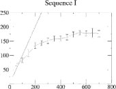
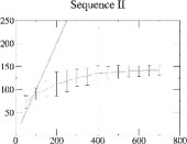
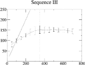
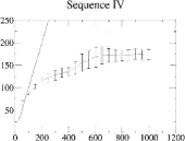
Figure 32: Integrated autocorrelation times of the plaquette together with their standard errors as a function of the differencing lag for the different update sequenced.

The Jackknife variances as a function of the bin size are displayed in Fig. 33. In all cases, plateaus can be identified. Note again, that there is no systematic control of the errors when using this method.

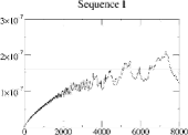
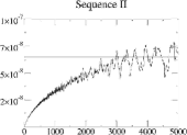
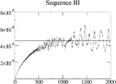
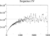
Figure 33: Jackknife variances as a function of the bin size for the different updating sequences.

The resulting autocorrelation times and the total numerical efforts (as computed from the lag-differencing method) are summarized in Tab. 12. The data for Sequence 0 has been taken from Tab. 6.

	$\mathbf{\tau_{\mbox{\tiny int}}}$ from LDM	Lag $\mathbf{l}$	$\mathbf{\tau_{\mbox{\tiny int}}}$ from Jackknife	Total effort/MV-Mults
Sequence 0	$334.3\pm 65.6$	-	$1441$	$342189$
Sequence I	$180.5\pm 8.3$	$>550$	$611.8$	$436070$
Sequence II	$141.4\pm 10.5$	$>400$	$318.0$	$397098$
Sequence III	$152.8\pm 10.1$	$350-600$	$109.8$	$498461$
Sequence IV	$175.2\pm 11.7$	$>700$	$129.7$	$393503$

Table 12: Integrated plaquette autocorrelation times from the lag-differencing and the Jackknife methods together with the total costs for a statistically independent configuration.

When examining the integrated autocorrelation times one finds that indeed some gain can be achieved by increasing the number of local gauge field sweeps. However, the effect clearly saturates already after as few as four consecutive sweeps have been performed in Sequence IV. On the other hand, increasing the number of boson field sweeps in Sequence III did not produce any practical gain.

In contrast, the picture is different if the total efforts are considered. Apparently a decrease in the autocorrelation time is accompanied by an increase in the effort for a single trajectory. From this finding one can conclude that one should better mix the local update sweeps. There is, however, one subtlety which is not reflected in Tab. 12: As it will be shown later in Tab. 14, on the APE-100 architecture a caching of the boson fields allows for an efficient implementation of subsequent gauge field sweeps. This would reduce the total cost in Sequence IV compared to Sequence 0 by the amount of three gauge field sweeps. The net effect of such an implementation is that the cost would only slightly increase for the execution of subsequent gauge field sweeps. Hence, one would find that for the APE-implementation an updating sequence like Sequence IV is superior to the sequence used previously.

In conclusion, the optimal updating sequence consists of a mixture of local gauge and boson field sweeps. One can update the gauge fields for several sweeps while holding the boson field background fixed. It does not appear to be efficient, however, to perform more than four gauge field sweeps in this way. In case the caching discussed in App. 9 is available, this method is indeed effective in reducing the total effort for a single trajectory, $E_{\mbox{\tiny MV-mults}}$, and hence also the total cost for a statistically independent configuration, $E_{\mbox{\tiny indep}}$.

3 Implementation Systems

The discussion so far has been limited to the machine-independent part of multiboson algorithms. In practical simulations, however, a particular architecture for the large-scale simulations has to be selected. This choice will have a considerable impact on the project since the complexity of a multiboson algorithm is huge compared to other algorithms in use today and the program is expected to run for several months.

For the purposes of this thesis, two platforms have been given major focus: The first platform was the APE-100 platform [231] which is also compatible with the APE-1000 [232] architecture. The machines used are installed at DESY/Zeuthen and at the Forschungszentrum Jülich in Jülich, Germany. The second target platform for the implementation was the ALiCE computer cluster [233] installed at Wuppertal University. In the following, the machines together with their specific merits and drawbacks will be presented. The properties of the implementations are discussed and the influence of the numerical precision on the calculations is examined.

1 APE Platform

The APE is a SIMD machine which executes a program in parallel on a number of nodes arranged in a three-dimensional mesh. The smallest configuration of nodes is a $2\times 2\times 2$-partition, the largest configuration available is an $8\times 8\times 8$-machine.

The APE-100 architecture can only execute single-precision floating point numbers efficiently in parallel. However, for special operations like global sums, a library for double-precision addition is available [234]. Given that a global sum only consumes a fraction of the total runtime of a program, there is no performance degradation to be expected. In contrast to floating point operations, integer calculations are being done globally on a single CPU (with no parallelization possible) with less efficiency. Especially integer operations on array indices should be kept at a minimum for the program to run efficiently. One further obstacle is the fact that the complete multi-boson program would be too large to fit into the memory of the machine — thus only a portion of the complete code can be written on the APE machines and the remaining parts must be run on conventional parallel computers.

One further problem is the bad I/O-performance of the machine. A save/restore of the complete machine state requires about $1$-$2$ hours of time (for a typical lattice of size $\Omega=32\times 16^{3}$ and $n_{1}=30-60$) which means that about $5-10\%$ of the whole runtime of a job (which is usually about $20-30$ hours) would be wasted for I/O operations. This problem can be overcome, however, by not storing the boson fields on disc, but rather performing a global heatbath thermalization sweep (see Sec. 4) to initialize them prior to a run. This strategy is more efficient (and also is more effective in terms of autocorrelation times of observables) than saving and restoring the complete machine state each time.

The compiler and optimizer technologies lag behind the industry standards of conservative parallel computers — the CPUs have no caches (only the registers of the floating point processors serve as a kind of $1$st level cache). Most optimization strategies (like loop unrolling, prefetching etc.) have to be implemented manually using the high-level language of the platform. This language is called TAO [235] and is a language build on Zz, which is a compiler construction language. However, due to the fact that Zz is still accessible (to extend the features of TAO and to implement manual loop-unrolling etc.), the system is effectively using a dynamic grammar, which is known to bear a lot of responsibility on the implementor. The drawback is that more complicated programs developed on the machine cannot easily be ported to different architectures and thus the maintenance costs will soon become a reasonable factor. This is no concern for trivial algorithms like the HMC, but will become a serious problem once a larger source code base is to be established on the machine.

One particular problem is that the sources of the compilers are not publicly available, meaning that bugs are hard to locate and fix compared to e.g. the GNU compilers. This implies that the development tools could not be run on modern and fast machines — the typical compile times during the early phases of the project were of the order of $20-30$ minutes resulting in turn-around times of more than half an hour.

The advantages of the APE architecture are that a lot of computer time is available and it has proven to be the ideal platform for simple algorithms like the HMC, which essentially rely only on the implementation of an efficient matrix-vector multiplication. Furthermore the platform scales very efficiently since the communicational overhead is minimal. This results in a rather small latency and is thus a counterpoint to the workstations clusters available today, see [236] for a different application of workstation clusters which demonstrates the same properties. Several of these shortcomings have improved with the advent of the APE-1000 architecture [232], but experience is still too sparse to include major results in this thesis. The APE-1000 architecture still has problems regarding the maximum machine size and the fact that double precision calculations will introduce a performance hit of a factor of four in the peak performance.

The first implementation of the TSMB algorithm used in this thesis has been written on the Q4open machine located at the NIC in Jülich, Germany. The machine had a configuration of $2\times 4\times 4$ nodes and served as the major development platform until Spring 2000. Sadly, it went out of service due to a defect board.

2 ALiCE Cluster

At a later stage of this project, development was shifted to the ALiCE computer cluster installed at Wuppertal University, where modern compilers and development tools are available. Most results have in fact been obtained on this machine. The cluster consists of $128$ Compaq DS 10 workstations, each equipped with a 21264 Alpha processor running at $616$ MHz. The size of the second level cache is $2$ Mbyte. The network is based on a Myrinet network with a peak performance of $1.28$ Gbit/$s$.

The coding done on this platform was immediately usable on other parallel machines, like the CRAY T3E located at the ZAM, Jülich and the Nicse-cluster which is also located at the NIC institute. The program has been proven to run also on a cluster of standard, Intel-based workstations installed at Wuppertal University. The network of these machines is based on standard Ethernet which made the installation not competitive from a performance point of view, but very attractive for development and debugging purposes. This illustrates the particular advantage of standard tools over proprietary solutions: although the hardware costs might be smaller (the situation might be less clear once development costs are included, however), the Total Cost of Ownership (TCO) may outweigh the former price. In fact, the total costs for maintenance and software may become larger than the pure hardware costs.

3 Accuracy Considerations and Test Suites

The complexity of code for the multiboson algorithm is high compared to the case of other algorithms in use today like the HMC. The multiboson code on the APE machine (together with the production environment) amounted to more than $11000$ lines of code; the program on the ALiCE cluster consisted of $17000$ lines of code (for the single-node and the parallel version) and the administrative software required another $17000$ lines. For the measurement of hadronic masses, a program with a size of $29000$ lines of code was required. This clearly asks for having efficient test suites available to track down possible sources of errors.

Local Fermionic Action

An important part of the program consists of the implementation of the fermionic action. Explicit forms of the different expressions required for the local action are given in App. 9. The local forms have to be consistent with the implemented matrix-vector multiplication. Then one can alter a single link at an arbitrary site and compare the results of Eqs. (69), (2) and (2). The second test consists of changing a single color-spinor with an arbitrary index $j$, $1<j\leq n_{1}$, and again comparing the results of (69) and (2). The residual error should only be limited by the machine precision. This can also act as a test on whether the single precision of the APE machines is a real limitation.

In fact, for the application of (2) one has to sum up $n_{1}$ terms in single precision to get a complex $3\times 3$ matrix which may introduce already difficulties at moderate values of $n_{1}$. To examine the errors as they occur in practical computations, one can already get along with a very small lattice since the major source of numerical errors occurs in the local update part. Therefore, a simulation has been performed using a thermalized configuration on a $\Omega=4^{4}$ lattice at the physical parameters given in Tab. 1 on the QH1-board at DESY/Zeuthen. The polynomial in question has been chosen to be $n_{1}=32$ with $[\epsilon,\lambda]=[3\times 10^{-3},3]$. The maximum numerical error in the three expressions is displayed in Figure 34, where the distribution of the inaccuracies are shown. They have been obtained by considering separately each site on a single node during a gauge field updating sweep. The error obviously is bounded from above and only scarcely exceeds $1\times 10^{-6}$. In the development phase such a plot turned out to be extremely useful since identifying the sites which give a huge numerical error can help to track down program bugs rather easily.

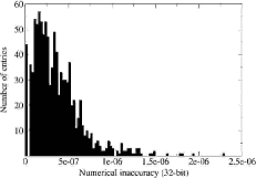
Figure 34: Maximum numerical error between the different implementations of the fermionic actions for local changes of the gauge field.

The second message to be learned from Fig. 34 is that the $32$-bit precision used is not an obstacle in actual simulations: The systematical error introduced by the local gauge field updates is obviously under control.

The same can be done for local changes of the boson field and considering the expressions Eqs. (69) and (2). The corresponding results are displayed in Fig. 35. Apparently, the same can be said about the boson field case as has been stated before in the gauge field case.

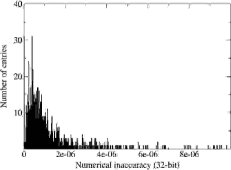
Figure 35: Maximum numerical error between the implemented actions for local changes of the boson field.

The Inverse Square-root

Another problem is posed by the residual error of the inverse square root required for the TSMB algorithm, Eq. (76). As has already been discussed in Sec. 1, the systematic error can be computed via (4) and must be less than one percent.

The question arises, how accurate the approximation can be at best. Given the fact that in case of the HMC algorithm one has a residual error of $2\%$ if one uses $32$-bit floating point numbers on an $\Omega=40\times 24^{3}$ lattice (see Sec. 2), the question arises, how large the lattice may be in the TSMB case if one only has access to single precision on a particular architecture. This question is answered by Fig. 36, where the residual error $\|\hat{R}_{n_{3}}^{n_{2}}(\tilde{Q}^{2})\|$ of the noisy correction step is plotted vs. the order of the third polynomial, $n_{3}$ (the polynomial $n_{2}$ has been chosen to be $n_{2}=160$). The calculation has been performed using both $32$-bit (single precision) and $64$-bit (double precision) algebra. The lattice sizes which have been considered were $\Omega=8^{4}$ and $\Omega=32\times 16^{3}$.

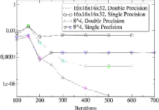
Figure 36: Residual error of the noisy correction $\|R_{n_{3}}^{n_{2}=160}(\tilde{Q}^{2})\|$ vs. the number of iterations $n_{3}$ for two lattice sizes. Both single ($32$ bit) and double precision ($64$ bit) have been used.

On the $\Omega=8^{4}$ lattice the results coincide up to orders of about $n_{3}=200$. Beyond this point, the single precision result deviates from the double precision curve. Finally, the single precision numbers saturate at $n_{3}\geq 250$. The accuracy which can be reached is still satisfactory since it is bounded by $\|\hat{R}_{n_{3}}^{n_{2}}(\tilde{Q}^{2})\|\approx 2.1\times 10^{-4}$. Hence, one can conclude that single precision is adequate on an $\Omega=8^{4}$ lattice.

On the $\Omega=32\times 16^{3}$ lattice, the single precision result saturates already at $\|\hat{R}_{n_{3}}^{n_{2}}(\tilde{Q}^{2})\|\approx 4.6\times 10^{-3}$. This is more than on the $\Omega=8^{4}$ lattice, but it is still sufficiently small. The double precision curve also shows a saturation, but not before $n_{3}=400$ and an accuracy of $\|\hat{R}_{n_{3}}^{n_{2}}(\tilde{Q}^{2})\|\approx 2.1\times 10^{-5}$ has been achieved. Again, this is completely acceptable.

The conclusion to be drawn from this test is that single precision arithmetic is not at all a problem on an $\Omega=8^{4}$ lattice, and is still acceptable on lattices as large as $\Omega=32\times 16^{3}$. On larger lattices, however, single precision may no longer be feasible and one should refrain from using $32$-bit arithmetics.

4 Architectures and Efficiency

All architectures discussed so far have certain advantages and disadvantages. In this section, the efficiencies of the implementations are compared against each other. Table 13 shows the execution times of the different parts of the multiboson implementations for a selection of architectures. The physical parameters of the runs are given in Tab. 1, while the algorithmic parameters are listed in Tab. 3 with $n_{1}=20$. The lattice size was again $\Omega=8^{4}$.

In case of the ALiCE cluster and the CRAY T3E, an eight-node partition with parallelization in $z$- and $t$-direction has been employed which results in local lattices of $\Omega_{\mbox{\tiny loc}}=2\times 8\times 8\times 4$. Table 13 displays the execution times of the different algorithms employed.The last line shows the ratio of local update sweeps to the global matrix-vector multiplications taking place in the noisy correction step. This is the key quantity of interest, where the influence of a particular architecture is most clearly exposed.

Algorithm	Time on ALiCE	Time on CRAY T3E
Mat-Vect. mult	$0.04938s$	$0.06542s$
Noisy correction	$17.777s$	$23.551s$
Boson heatbath	$1.10352s$	$4.02112s$
Boson overrel.	$1.06641s$	$3.79800s$
Gauge heatbath	$1.17969s$	$4.12083s$
Ratio local/global	$0.3748$	$1.0045$

Table 13: Execution times of several parts of the TSMB algorithm on the ALiCE cluster and the CRAY T3E.

For the APE-100, an eight-node Q1 board has been used with a lattice size of $\Omega=4^{4}$. The local lattices were $\Omega_{\mbox{\tiny loc}}=2\times 2\times 2\times 4$ per node. The resulting execution times of these algorithms are quoted in Tab. 14. In contrast to the above implementation, the APE program uses an efficient caching strategy, where the contributions of the boson fields to the local staples, Eq. (2), which are unchanged by a gauge field sweep are held in memory, see App. 9 for details. This allows to reduce the computational costs for repeated local gauge field sweeps. The time required for the initialization of the gauge field sweep is given in the fifth line of Tab. 14. This strategy has only been implemented on the APE, but in principle this caching scheme is machine-independent and could also be implemented in the other program.

Algorithm	Time
Mat-Vect. mult	$0.01354s$
Noisy correction	$4.876s$
Boson heatbath	$1.634s$
Boson overrel.	$1.482s$
Init gauge sweep	$1.695s$
Gauge heatbath	$0.124s$
Ratio local/global	$1.6503$

Table 14: Execution times of the parts of the TSMB algorithm on an APE board.

When comparing the ALiCE and the CRAY T3E, one realizes that the CRAY T3E architecture has a more efficient network, but lacks the large second-level caches of the ALiCE nodes. This explains why the communication-intensive performance of the matrix-vector multiplication is very efficient on the CRAY T3E. On the other hand, the local update sweeps are very cache intensive and communication between nodes only plays a minor role. Therefore, the local update sweeps contribute a much smaller fraction to the total runtime on the ALiCE cluster, while they account for about $50\%$ of the total sweep time on the T3E.

The APE-100 architecture shows an even more prominent dominance of the local update sweeps, which consume about $2/3$ of the total runtime. This can be attributed to the fact that the CPUs have no second-level cache at all and the data has to be fetched from memory each time. Therefore the local update sweeps are rather inefficient, while the global matrix-vector multiplications are very efficient.

4 Summary

The TSMB algorithm requires three approximations to an inverse power of the Hermitian Wilson matrix. All approximations are being performed with static inversion algorithms as discussed in Sec. 1. The first is a crude approximation to an inverse power of $\tilde{Q}^{2}$ with order $n_{1}$. The second is a refined approximation to the same function with order $n_{2}$. The third one approximates the inverse square root of the polynomial with which the second approximation is performed.

The best method to find the first polynomial consists of applying the GMRES algorithm (see Sec. 3) to one or more thermalized gauge field configurations at the physical point one is interested in. This method is limited by the numerical precision of the architecture used to generate the polynomial. The other method consists of using a quadratically optimized polynomial. The latter choice only requires rough knowledge of the spectral bounds.

The second and third polynomials have to be quadratically optimized polynomials. The value of $\epsilon$ for the product of the first and the second polynomial should be chosen such that it is slightly smaller than the average smallest eigenvalue. Its order has to be adjusted such that the reweighting factor is not fluctuating more than a few percent. Since the convergence is exponential, this can be achieved without too much effort.

The third polynomial must have a sufficiently high order such that its corresponding determinant norm, Eq. (4), or rather the resulting systematic error, Eq. (7), is never exceeding values of $\simeq 10^{-3}$.

The order of the first polynomial influences the acceptance rate of the correction step. It appears to be safe to make the acceptance rate somewhat smaller than $50\%$. The motion in phase space depends linearly on the number of boson fields. The decreased acceptance rate counteracts the increased mobility in phase space and the resulting efficiency does not appear to depend on the acceptance rate. Since the numerical cost of a single trajectory is proportional to the number of boson fields, the total cost for a statistically independent gauge field configuration, Eq. (11), is then given by

$$E_{\mbox{\tiny indep}}\propto n_{1}^{2}\,.$$ (12)

This formula should apply for runs at different parameters and different orders $n_{1}$ if the acceptance rates are held constant and if the field updates dominate the time needed for a single trajectory.

A trajectory is given by the updating sequence, i.e. the transition function of the Markov chain. It consists of a number of update sweeps for the boson fields and local update sweeps of the gauge field. It has turned out that the boson field updates should be mixed with the gauge field updates, but a number of subsequent gauge field updates allows a similarly efficient decorrelation. Each trajectory is completed by a noisy correction step. In view of the fact that the acceptance rate is rather independent from the local gauge field updates, the optimal efficiency can be achieved by performing a larger number of local gauge field updates between two noisy corrections. Thus, the sequence should be arranged in such a way that the field updates dominate the total runtime.

Furthermore, it is important to identify the machine architecture which meets the specific demands of MB algorithms. While a conventional massive-parallel machine with a network similar to the CRAY architecture, but small caches on the nodes does not perform well with respect to the local update sweeps, its efficient network allows for a rather efficient matrix-vector multiplication. However, as it has been discussed in Sec. 4, one can (and, in fact, one should) always arrange the updating sequence in such a manner that the local updating sweeps dominate the total runtime of the code. Hence, the machine best suited for TSMB calculations is found to be a cluster of workstations with large cache and standard programming tools.

The APE-100 system does not perform very well in the local update sweeps and suffers from the problem that the coding of the algorithm can until now not be used on any other machines. The former problem may be overcome with the advent of the APE-1000 architecture which may (due to the large number of CPU registers) reduce the number of memory accesses required. The latter problem can not be expected to be solved before the advent of the APE-Next platform [237]. Due to the complexity of the algorithm it appears reasonable to implement first a reference implementation in a standard language on a different architecture before starting with the coding on the APE platform.

There is still room for further improvements, however. In particular, improving the approximation scheme of the third polynomial would allow to overcome the limitations of the current implementations and should make the algorithm applicable to larger lattices even with single precision arithmetics. A different place where further improvements are in order is the first polynomial. Although the optimal way to find its coefficients has been identified, this method still requires high numerical accuracy of the implementation system.

Chapter 4 Comparison of Dynamical Fermion Algorithms

In the first section, Sec. 1, the variant of the multiboson algorithm with TSMB correction step, which has been studied in detail in Chapter 3, is applied at different physical locations in parameter space. At all points, results from the HMC method are available. This allows for a direct comparative study.

Section 2 directly compares the efficiencies of MB algorithms with that of the HMC. This investigation is not limited to the MB-variant discussed so far, but also covers the non-Hermitian variant with UV-filtering and gauge field overrelaxation as proposed by de Forcrand in [220] (cf. Sec. 3). These results might be of importance for future simulations of gauge theories with dynamical fermions, see e.g. [238]. The study is carried out on equal lattice volumes and with identical physical parameters. Hence, it will allow to probe the scaling of the algorithms as the continuum limit is approached.

1 Simulation Runs at Different Parameters

The TSMB variant of the multiboson algorithm is applied to situations at different physical points in parameter space with two dynamical fermion flavors. A direct comparison with the HMC algorithm is given. The latter acts as a benchmark for the alternative proposals.

The HMC simulations have all been carried out on volumes $\Omega=32\times 16^{3}$. The physical parameters of the various runs performed here and in the rest of this chapter are compiled in Tab. 1 and have been taken from [148], see also [228, 227]. The second line is identical to Tab. 1 in Chapter 3.

Bare parameters			Physical parameters
$\mathbf{N_{f}^{\mbox{\tiny sea}}}$	$\mathbf{\beta}$	$\mathbf{\kappa}$	$\mathbf{(am_{\pi})}$	$\mathbf{(am_{\rho})}$	$\mathbf{m_{\pi}/m_{\rho}}$	$\mathbf{a}$/fm
$2$	$5.5$	$0.158$	$0.5528(40)$	$0.6487(55)$	$0.8522(95)$	$0.166$
$2$	$5.5$	$0.159$	$0.4406(33)$	$0.5507(59)$	$0.8001(104)$	$0.141$
$2$	$5.5$	$0.160$	$0.3041(36)$	$0.4542(78)$	$0.6695(138)$	$0.117$
$2$	$5.6$	$0.156$	$0.4464(27)$	$0.5353(42)$	$0.8339(66)$	$0.137$

Table 1: Bare and physical parameters for the comparison between HMC and TSMB. Also cf. Sec. 1.

The multiboson algorithm has been operated on rather small lattices with volumes $\Omega=8^{4}$ and $\Omega=16\times 8^{3}$. Measurements of the physical masses can be expected to differ from those on the larger volumes due to finite-size effects [148]. Hence, runs on such small lattice sizes can only be preliminary studies which need to be supplemented later by runs on larger volumes. The quantity under consideration here is the average plaquette. This observable will exhibit only a weak dependence on the lattice volume. These runs corroborate the tests performed in Sec. 3 of Chapter 3.

Table 2 gives the total statistics in numbers of trajectories entering the analysis. The complete data set as given in Tab. 4 has been exploited, therefore the statistics in this particular case is enormous. Furthermore, the machines on which the data have been sampled are shown.

Bare parameters
$\mathbf{\beta}$	$\mathbf{\kappa}$	Volume $\mathbf{\Omega}$	Machine	Algorithm	Trajectories
$5.5$	$0.158$	$8^{4}$	ALiCE cluster	TSMB	$17703$
$5.5$	$0.158$	$32\times 16^{3}$	APE-100 QH4	HMC	$3042$
$5.5$	$0.159$	$8^{4}$	ALiCE cluster	TSMB	$448055$
$5.5$	$0.159$	$32\times 16^{3}$	APE-100 QH4	HMC	$4518$
$5.6$	$0.156$	$16\times 8^{3}$	APE-100 Q4	TSMB	$4424$
$5.6$	$0.156$	$32\times 16^{3}$	APE-100 QH2	HMC	$4697$

Table 2: Machines and statistics for the test runs at different physical parameters.

Table 3 lists the resulting values for the average plaquette together with their standard errors for the different algorithms used. The standard errors have been obtained using the Jackknife method on the plaquette time series.

Bare parameters
$\mathbf{\beta}$	$\mathbf{\kappa}$	Plaquette/HMC	Plaquette/TSMB
$5.5$	$0.158$	$0.55546(6)$	$0.55380(41)$
$5.5$	$0.159$	$0.55816(4)$	$0.55909(27)$
$5.6$	$0.156$	$0.56988(2)$	$0.56865(86)$

Table 3: Average plaquette values with their standard errors obtained from the different samples.

The plaquette values obtained with the HMC coincide with those generated by the TSMB algorithm up to three digits.

In conclusion, the TSMB implementation indeed produces identical plaquettes. This comparison demonstrates the correct implementation and the correct execution of the MB algorithm.

2 Efficiency of Multiboson Algorithms

In this section, three different algorithms for the simulation of Lattice QCD with two dynamical fermion flavors are compared. The physical parameters are the ones given in the second line of Tab. 1. In all cases, the lattice volume has been chosen to be $\Omega=32\times 16^{3}$. This allows for a measurement of hadronic masses and opens the stage for a direct comparison of both algorithms.

The HMC algorithm has been introduced in the previous section, see Tab. 2. The two variants of MB algorithms used are the implementation with quadratically optimized polynomials discussed in the previous section Sec. 1 and an implementation based on the UV-filtered non-Hermitian approximation. The latter code has been written by M. D’Elia and Ph. de Forcrand. Both programs have been implemented on the APE-100 QH4 installed at DESY/Zeuthen. While the former variant uses heatbath sweeps for the gauge field updates (it will be called “MB-HB” in the following) and the TSMB correction step, the latter uses overrelaxation sweeps (in the following abridged with “MB-OR”) for the gauge field and an exact correction step. To reflect the different updating strategies used, the algorithms are named after the corresponding local gauge field updates.

1 Tuning the MB-HB Algorithm

For the MB-HB algorithm, the question arises how the acceptance rate of the correction step changes with the volume and what the consequences for the polynomial orders are. Table 4 shows two different choices of parameters and the corresponding acceptance rates. Thus, the choice $n_{1}=60$ gives an acceptance rate of about $50\%$, while for smaller values of $n_{1}$ the acceptance rate is decreasing rather fast. We observe a significant volume dependence since in the case $\Omega=8^{4}$ one only needs $n_{1}=20$ to get similar acceptance rates (consult Tab. 4). For the simulation run to be presented below the parameters from the second line have been taken.

Algorithmic parameters
$\mathbf{n_{1}}$	$\mathbf{n_{2}}$	$\mathbf{n_{3}}$	$\mathbf{[\epsilon,\lambda]}$	Acc. rate
$42$	$160$	$250$	$[7.5\times 10^{-4},3]$	$15.2\%$
$60$	$150$	$250$	$[6\times 10^{-4},3]$	$49.4\%$

Table 4: Different polynomial parameters and the resulting acceptance rates for the MB-HB algorithm.

The updating strategy is shown in Tab. 5 and is chosen similar to Tab. 3 in the previous chapter. Note, as has been discussed in Sec. 4, the boson fields do not have to be restored if the correction step rejects a proposed gauge field configuration.

Updates/Trajectory

$1$ boson HB, $3$ boson OR, $2$ gauge heatbath, $1$ noisy corr.

Table 5: Updating sequence for the MB-HB algorithm.

The heatbath algorithm (cf. Sec. 2) has been employed for the gauge field updates. It is important to notice that a single-hit heatbath algorithm is sufficient if the scheme from [157] is used. In fact, acceptance rates exceeding $99\%$ have been observed when generating the distribution for $a_{0}$ (consult Sec. 2 for the notation).

In the version of the program employed, the contribution of the unit-submatrix from the even points in the noisy vectors has been included in the noisy correction step. This resulted in a systematic error of about $2.48\%$ when applying Eq. (7). If this had not been done, one could have reduced the polynomial orders $n_{2}$ and $n_{3}$. We do expect this to influence neither the stochastic averages nor the autocorrelation times in terms of sweeps, however.

2 Tuning the MB-OR Algorithm

In contrast to the former variant, the other MB algorithm does not make use of a polynomial approximation in the correction step but makes an adaptive inversion. As has been discussed in Sec. 3, this requires a nested iteration of an adaptive inversion and the polynomial $P_{n_{1}}$, which acts as a preconditioner. This approach has the great practical advantage that no multicanonical reweighting for the measurement of observables is necessary, but has the shortcoming that one has an increased effort once configurations with exceptionally small eigenvalues are encountered. In the present case, however, we do not expect this to have a major influence.

The power of the GMRES polynomials in conjunction with UV-filtering for the non-Hermitian Wilson matrix is demonstrated if one considers the order of the polynomial $P_{n_{1}}(\cdot)$ required to arrive at an acceptance rate of $60.3\%$. The polynomial needed in this case has an order of only $n_{1}=24$.

Thus, the number of boson fields could have been reduced by a factor of $2.5$ (and even more if one aims for an acceptance rate of about $50\%$). This number takes into account the combined effect of using the non-Hermitian Wilson matrix, employing the expansion of Eq. (95), and using the GMRES algorithm instead of quadratically optimized polynomials. To actually find this polynomial, however, a thermalized gauge field configuration had to be provided from the HMC run. Had this configuration not been available prior to the run, the run would have had to be performed with a non-optimal polynomial instead for thermalization. This would have increased the total investment into the algorithm.

Updates/Trajectory
$1$ gauge OR, $5\times\left(\right.$ $1$ boson OR, $1$ gauge OR $\left.\right)$,
$1$ boson field global quasi-HB,
$5\times\left(\right.$ $1$ gauge OR, $1$ boson OR $\left.\right)$, $1$ gauge OR,
$1$ noisy corr.

Table 6: General algorithmic parameters for MB-OR run.

The precise update sequence for a single trajectory is given in Tab. 6. In contrast to the former multiboson implementation discussed in Sec. 1, only overrelaxation sweeps (see Sec. 3) have been used for the gauge field. Although this algorithm alone is non-ergodic, ergodicity is ensured by the boson field global quasi-heatbath (this method has been discussed in Sec. 2). In particular, instead of only two gauge field updates between a correction step, in total $12$ gauge field updates are being run. However, the mixing of gauge and boson field updates requires to restore both kinds of fields in case the correction step rejects the current configuration. This results in much larger memory requirements. As has been argued in Sec. 4, one can expect that this updating sequence results in a faster decorrelation than the updating sequence in Tab. 5.

In conclusion one can expect that the MB-OR implementation may perform better since both the number of boson fields is reduced significantly and the updating sequence ensures a faster decorrelation.

3 Direct Algorithmic Comparison

The observables under consideration were the average plaquette, the (non-singlet) pseudoscalar meson mass (denoted as pion $\pi$) and the (non-singlet) vector meson mass (denoted as rho-meson $\rho$). Their expectation values (for the three different algorithms) together with their standard errors are shown in Tab. 7. The hadronic masses have been taken from Orth [148].

Algorithm	Trajectories	Configurations	Plaquette	$\mathbf{(am_{\pi})}$	$\mathbf{(am_{\rho})}$
HMC	$3521$	$140$	$0.55816(4)$	$0.4406(33)$	$0.5507(59)$
MB-HB	$5807$	$108$	$0.55819(6)$	$0.448(10)$	$0.578(17)$
MB-OR	$6217$	$177$	$0.55804(7)$	$0.4488(37)$	$0.5635(83)$

Table 7: Average plaquette and hadronic masses for the three different sampling algorithms for Lattice QCD used.

The plaquette values agree within errors, while the meson masses agree within at most two standard deviations. The statistics for the MB-HB algorithm is worse than in the other cases.

Table 8 shows the resulting total efforts as defined in Eq. (11) for the three algorithms employed. The quantities under consideration are the meson masses. The efforts have been computed by Orth in [148] using the Jackknife method. See also [239] for the latest results.

	Efforts for meson masses
Algorithm	$\mathbf{E_{\mbox{\tiny indep}}(m_{\pi})/\mbox{MV-mults}}$	$\mathbf{E_{\mbox{\tiny indep}}(m_{\rho})/\mbox{MV-mults}}$
HMC	$<810000$	$<810000$
MB-HB	$>2000000$	$>2000000$
MB-OR	$264000$	$352000$

Table 8: Numerical efforts for meson masses obtained by employing three different sampling algorithms. Courtesy B. Orth.

Finally, the plaquette is investigated. The time series for the HMC method at these physical parameters has already been examined in Sec. 1. Figures 1 (this figure is identical to Fig. 12), 2 and 3 show the autocorrelation functions and the corresponding autocorrelation times computed for the plaquette histories from the HMC, the MB-HB and the MB-OR algorithms respectively.

Figure 1: Autocorrelation function and the corresponding integral as a function of the cutoff for the plaquette history from the HMC run. This figure is identical to Fig. 12.

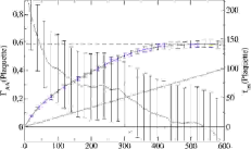
Figure 2: Autocorrelation function and integrated autocorrelation time for the plaquette histories of the MB-HB algorithm.

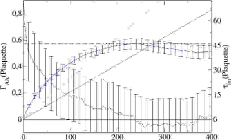
Figure 3: Autocorrelation function and integrated autocorrelation time for the plaquette histories of the MB-OR algorithm.

The efforts for each single trajectory, the corresponding autocorrelation times, and the total efforts to obtain one statistically independent plaquette measurement are listed in Tab. 9. Note that — as has been pointed out in Sec. 1 — the effort for a single trajectory could have been reduced in the case of the MB-HB algorithm. The integrated autocorrelation times have been determined using the windowing procedure which has been discussed in Sec. 5.

Algorithm	Effort/Trajectory	$\mathbf{\tau_{\mbox{\tiny int}}(\mbox{{Plaquette}})}$	$\mathbf{E_{\mbox{\tiny indep}}(\mbox{{Plaquette}})/\mbox{MV-mults}}$
HMC	$16200$	$11.0\pm 0.4$	$356400\pm 12960$
MB-HB	$2000$	$141.8\pm 32.7$	$567200\pm 130800$
MB-OR	$4400$	$44.7\pm 3.4$	$393360\pm 29920$

Table 9: Autocorrelation times and efforts for independent plaquette measurements for the three different algorithms at $\beta=5.5$ and $\kappa=0.159$.

The time series from the HMC algorithm contains $320$ autocorrelation times which is sufficient to obtain a reliable estimate for the autocorrelation time. The MB-OR algorithm was run for $140$ autocorrelation times, which should be enough for a good estimate. The MB-HB algorithm, however, has only accumulated of the order of ${\cal O}(40)$ autocorrelation times if the value of $\tau_{\mbox{\tiny int}}$ is correct. This is too short for a safe determination of $\tau_{\mbox{\tiny int}}$, therefore, these numbers have to be taken with a grain of salt. One cannot be sure that already the longest mode has been measured in the time series, but one can consider the autocorrelation mode giving rise to this value as a lower limit of the true autocorrelation time.

As it has already been anticipated, the MB-HB algorithm can not compete with the MB-OR algorithm at this point in parameter space. The observed autocorrelation time for the plaquette in terms of trajectories is a factor of about $3.2$ larger than for the MB-OR algorithm. However, the statistics which went into the MB-HB run is not yet sufficient. Given the large difference in the number of boson fields and the small number of gauge field updates between the noisy corrections during each trajectory compared to the MB-OR algorithm, the efficiency may consequently be even worse than what is expressed in Tab. 9. The results for the meson masses (cf. Tab. 8) are compatible with the these findings. Again, the numbers should only be considered to be lower limits and may not capture the longest mode of the time series in question.

When comparing the MB-OR and the HMC algorithms regarding the plaquette autocorrelation times, one finds that the algorithms are similarly efficient. In the case of the meson masses, the problem occurs that for the HMC only the configuration at every $25$th trajectory has been analyzed. There is no residual autocorrelation in the sample, therefore the actual autocorrelation times may be even smaller than the numbers given in Tab. 8.

In conclusion, at the physical point given in Tab. 1, the MB-OR algorithm performs for the decorrelation of the hadronic masses at least as good as the HMC. For the measurement of hadronic masses, the results are similar. However, one finds that the tuning of MB algorithms is crucial for their performance.

4 Scaling Behavior of Algorithms

The ultimate goal of Lattice QCD simulations has been formulated in [10] (cf. Sec. 3), namely the demand to simulate with three light fermionic flavors at quark masses of about $1/4m_{s}$. For this goal to be reached, an algorithm is required which has a sufficiently weak critical scaling exponent when approaching the chiral regime (see Eq. (22)). The challenge is now to apply the algorithms from the previous comparison to a point in phase space with lighter fermion masses. The point has been chosen from the third line in Tab. 1, i.e. $\beta=5.5$ and $\kappa=0.160$. It corresponds to lighter quark masses and should allow to shed some light on the scaling behavior of the algorithms under consideration.

The updating sequence of the multiboson algorithm has been chosen identical to the previous run, see Tab. 6. The number of boson fields had to be increased, however, and is now $n_{1}=42$. This results in an acceptance rate of $65.85\%$.

As has been found in Eq. (12), the total cost for a single trajectory should depend quadratically on the number of boson fields, $n_{1}$. From the cost obtained in Tab. 9 for $n_{1}=24$ we read off that an estimate for the cost with $n_{1}=42$ is given by

$$E_{\mbox{\tiny indep}}\simeq\left(\frac{42}{24}\right)^{2}\times 393360\pm 29920=1204665\pm 91630\,.$$ (1)

This estimate neglects the non-quadratic contribution of the correction step to the trajectory, but should still be a good approximation given the fact that the updating sweeps dominate the total cost.

The number of trajectories performed in each case together with the average plaquette is listed in Tab. 10. The plaquettes coincide within their standard errors.

Algorithm	Trajectories	Plaquette
HMC	$5003$	$0.56077(6)$
MB-OR	$9910$	$0.56067(5)$

Table 10: Statistics and average plaquette for the HMC and the MB-OR algorithms at $\beta=5.5$ and $\kappa=0.160$.

The autocorrelation functions corresponding to the plaquette histories are displayed in Figs. 4 and 5.

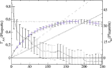
Figure 4: Autocorrelation function and integrated autocorrelation time for the plaquette histories of the HMC algorithm.

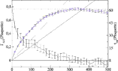
Figure 5: Autocorrelation function and integrated autocorrelation time for the plaquette histories of the MB-OR algorithm.

The corresponding efforts for a single trajectory, the integrated autocorrelation times for the plaquettes and the resulting efforts are given in Tab. 11. The statistics for the HMC algorithm are now more than $140$ autocorrelation times, while the MB-OR has generated about $160$ autocorrelation times. These numbers should allow for a reliable estimate of the efficiencies in both cases. In addition, the cost estimate from Eq. (1) is in excellent agreement with the measured effort $E_{\mbox{\tiny indep}}$ in Tab. 11.

Algorithm	Effort/Trajectory	$\mathbf{\tau_{\mbox{\tiny int}}(\mbox{{Plaquette}})}$	$\mathbf{E_{\mbox{\tiny indep}}(\mbox{{Plaquette}})}$
HMC	$42000$	$34.1\pm 3.1$	$2864400\pm 260400$
MB-OR	$8800$	$61.1\pm 4.1$	$1075360\pm 72160$

Table 11: Autocorrelation times and efforts for independent plaquette measurements for the two algorithms at $\beta=5.5$ and $\kappa=0.160$.

In light of these results, it is clear that the MB-OR gained a lot of ground in comparison to the HMC. For the former, the total effort to generate one statistically independent configuration only increased by a factor of about $2.7$, while for the latter the effort has increased by a factor of $8.0$. The MB algorithm has become an overall factor of almost three more effective than the HMC. For the simulation of two light, degenerate fermion flavors, the algorithm of choice is therefore definitely a multiboson algorithm.

3 Summary

It has been shown that all implementations of MB algorithms considered indeed produce the same physical results as the HMC algorithm. However, MB algorithms are more complicated to operate and tune and it has turned out that a suboptimal choice can easily lead to a degradation in performance. The efficiency of MB algorithms depends strongly on the polynomial and the updating sequence. The optimal setup for the polynomial at the chosen working points has been identified in Sec. 2. Furthermore, it has been discussed in Sec. 4 that one should apply sufficiently many gauge field updates between the correction steps to ensure a fast decorrelation. In this way, the field updates will dominate the runtime of the algorithm and lead to an optimal exploitation of resources.

For intermediate quark masses the HMC is able to perform equivalently to a well-tuned multiboson algorithm. When going to lighter quark masses, however, the MB will pretty soon outrival the HMC. It still remains to be seen, to what extend a non-Hermitian polynomial approximation is a viable candidate for further simulations in the deep chiral regime as they are planned in [238]. One may have to switch to a Hermitian approximation after one starts to encounter “exceptional” configurations with negative real eigenvalues to get reasonable acceptance rates. This step might be accompanied with an increase of $n_{1}$. However, first indications regarding the behavior of the smallest real eigenvalues in simulations in the deep chiral regime are given in [240] and references therein. These preliminary results hint that in actual simulations the sign problem may be absent unless one gets extremely close to the chiral limit.

The optimal tuning of the MB algorithm can only be found after a certain runtime has already been invested since the best polynomial approximating the fermionic contribution to the action can only be gained from one or more thermalized gauge field configurations. This additional effort requires more logistics and should also be considered when estimating the efficiencies.

Due to the price in complexity one has to pay, the HMC can consequently still be the preferred choice whenever it can be expected to be comparable or only slightly inferior to MB algorithms. Nonetheless, for simulations at very light quark masses close to the physical regime, it cannot be expected that the HMC is competitive anymore. An excellent candidate for future simulations at such masses is therefore the MB algorithm.

Chapter 5 Exploring the Parameter Space with Three Degenerate Dynamical Flavors

Up to this point, the emphasis has been put on the simulation of two degenerate dynamical fermion flavors. However, as has been argued in Sec. 3, realistic numerical simulations of Lattice QCD require a simulation with three dynamical fermionic degrees of freedom. Reference [10] shows that it is sufficient to concentrate first on the case of three mass-degenerate dynamical fermion flavors with dynamical quark masses of the order of $1/4m_{s}$. One possible goal is to obtain the Gasser-Leutwyler coefficients from those runs. However, such an endeavor requires lattice sizes and Wilson-matrix condition numbers beyond what we are capable of handling today.

In this section, a first step in such type of program will be taken, namely the application of a multiboson algorithm with TSMB correction step to this physically interesting situation.

In order to prepare the stage, we will work on $\Omega=8^{4}$ and $\Omega=16\times 8^{3}$ lattices. This will help to acquire some insight onto the chances of doing more realistic simulations on $\Omega=32\times 16^{3}$ lattices, as previously carried out for $N_{f}=2$ in the SESAM-project [228, 133]. So the question is whether, in the $N_{f}=3$ scenario, we can establish an operational window to achieve a reasonably large pion correlation length without hitting the shielding transition that has been found in $N_{f}=2$ at finite volumes and fixed $\beta$, as $\kappa$ was increased towards $\kappa_{\mbox{\tiny crit}}$.

Section 1 gives a short overview of the determination of the non-zero temperature crossover and the shielding transition. It is important to avoid this region in parameter space since the physical properties of the non-hadronized region are different from the zero-temperature phase of QCD. In particular, no hadrons are expected to exist and consequently one cannot extract useful information on their masses.

The physically interesting point in parameter space in an infinite lattice volume $\Omega\rightarrow\infty$ is the critical point where the Wilson matrix describes massless fermions. This property has been discussed in Sec. 4. The practical ways to find this chiral limit are reviewed in Sec. 2.

The application to two different values of $\beta$ is discussed in Sec. 3. These runs have been performed with the TSMB algorithm and might allow to identify a potential working point for future simulations.

At this stage we would like to mention some previous algorithmic work on $N_{f}=3$ physics, which was mainly carried out at finite temperatures. Reference [241] presents a detailed study of the thermodynamical properties of three flavor QCD. It employs the $R$-algorithm for the numerical simulations.

Note that, algorithmically, extensions of the HMC can also be used for these kinds of simulations [186, 188, 189, 242].

1 The Non-Zero Temperature Crossover

It is expected that the phase space of QCD contains a “deconfined phase”, where chiral symmetry is restored and the quarks and gluons form a plasma with color-charges being Debye-screened. This transition takes place at some critical temperature. For general introductions to this topic consult [24, 32]. This phase is interesting for the description of hadronic matter at high temperatures and densities. However, when performing simulations relevant for the low-temperature phase of QCD — where the phenomenology is dominated by hadronized particles — this phase should be avoided.

This transition is accompanied by a jump in the free energy of the system. An order parameter is given by the Polyakov loop, which is defined to be [243]:

$$P(\vec{x})=\frac{1}{3}\frac{1}{L_{s}^{3}}\;\mbox{Tr}\,\prod_{x_{0}}^{L_{0}}U_{0}\left((x_{0},\vec{x})\right)\,,$$ (1)

with $\vec{x}$ being a point in three-space, and $L_{s}$ and $L_{0}$ the spatial and temporal lattice sizes, respectively. The physical picture of $P(\vec{x})$ is the description of the average world line of a static quark. Information about the free energy of a static quark-antiquark pair can be obtained from the correlation of two such loops having opposite direction

$$\Gamma(\vec{x},\vec{y})=\langle L(\vec{x})L^{\dagger}(\vec{y})\rangle\,.$$ (2)

One can show [32] that this quantity is related to the free energy $F_{q\bar{q}}(\vec{x},\vec{y})$ of a static quark-antiquark pair via

$$\Gamma(\vec{x},\vec{y})=\exp\left[-\beta F_{q\bar{q}}(\vec{x},\vec{y})\right]\,.$$ (3)

Assuming that $\Gamma(\vec{x},\vec{y})$ satisfies clustering, one finds

$$\Gamma(\vec{x},\vec{y})=\langle L(\vec{x})L^{\dagger}(\vec{y})\rangle\buildrel|\vec{x}-\vec{y}|\rightarrow\infty\over{\rightarrow}|\langle L\rangle|^{2}\,.$$ (4)

Hence, one obtains that if $\langle L\rangle=0$, the free energy increases for large $|\vec{x}-\vec{y}|$ with the separation of the quarks. This is a signal for the hadronization phase.

Therefore the order parameter indicates the phase of the system via

$$\langle P\rangle=\left\{\begin{array}[]{rl}=0&\mbox{hadronization}\;,\\ \neq 0&\mbox{finite-temperature phase}\;.\end{array}\right.$$ (5)

This argumentation so far is only valid in the absence of dynamical quarks. It may, however, also be extended to the case of dynamical quarks with finite mass, see [32]. In this case, the Polyakov loop might similarly indicate the non-zero temperature crossover.

Up to this point, the discussion has always considered the case where the temporal lattice extension is smaller than the spatial one, $L_{0}<L_{s}$. In actual simulations, the situation can also arise that a transition similar to the non-zero temperature crossover occurs for too small lengths $L_{s}$, even if $L_{0}$ is sufficiently large. In this case, one is similarly unable to measure hadronic masses properly. This phenomenon is called the shielding transition.

2 The Chiral Limit

Of particular importance for any simulation of QCD is the critical line in parameter space, where the mass of the pion vanishes. The vicinity of this point allows for a treatment using $\chi$PT, as it has been argued in Sec. 3. As explained in Sec. 4, the Wilson matrix then contains a zero-mode.

The critical line can be found by varying the hopping parameter $\kappa$ appearing in the action Eq. (89) at a fixed value of the gauge bare parameter $\beta$. Then one has to find the critical value $\kappa_{\mbox{\tiny crit}}$, where the fermionic contribution to the action describes massless fermions. Repeating this procedure for several values of $\beta$ yields the critical line in parameter space. This procedure is impeded once the shielding transition sets in.

A qualitative illustration of the shielding transition and the critical behavior is given in Fig. 1. The figure shows the squared pseudoscalar meson mass, $(am_{\pi})^{2}$, at a fixed value of $\beta$, as a function of $1/\kappa$. The solid curve shows the mass in the infinite volume limit, $\Omega\rightarrow\infty$. The dotted line corresponds to a correlation length $\xi_{\pi}^{2}=1/(am_{\pi})^{2}=1$.

As has already been pointed out, finite-size-effects (FSE) will induce the shielding transition which might inhibit a reliable extraction of zero-temperature physics. We illustrate this scenario by sketching the FSE for two different volumes, $\Omega^{(1)}<\Omega^{(2)}$, with lengths $L_{s}^{(1)}<L_{s}^{(2)}$. When measuring the mass on the smaller lattice volume, $\Omega^{(1)}$, one finds that the curve can be followed reliably up to the point $\kappa_{\mbox{\tiny shield}}^{(1)}$. Beyond this point, the shielding transition sets in and the mass can no longer be measured correctly on the smaller volume. The larger lattice volume, $\Omega^{(2)}$, allows to go closer to the critical point, but will still run into finite-size-effects at some higher value, $\kappa_{\mbox{\tiny shield}}^{(2)}$. The “true” value of $\kappa_{\mbox{\tiny crit}}$ (as defined in the limit $\Omega\rightarrow\infty$) can be estimated the better the larger the available volume.

Figure 1: Sketch of the FSE-induced shielding transition. The squared pseudoscalar meson mass, $(am_{\pi})^{2}$, is plotted vs. the inverse hopping parameter $1/\kappa$.

Lattice results become meaningful, once the pseudoscalar correlation length, stays larger than unity, $\xi_{\pi}\gg 1$. This condition is impossible to fulfill on the lattice $\Omega^{(1)}$ — the shielding transition sets in before the desired parameter region is reached. On the lattice $\Omega^{(2)}$, however, it is in fact possible to go beyond $\xi_{\pi}>1$ before shielding is observed. Hence, for a given set of parameters one has to increase the lattice volume until one reaches a “window”, where the FSE are under control while the mass already became sufficiently small.

But how to estimate $\kappa_{\mbox{\tiny crit}}$? On a given large enough lattice, one can use the following recipes (see also Sec. 4)

1. the point in $\kappa$-space where the condition number of the Hermitian Wilson matrix $\tilde{Q}$ diverges,

2. the point where the smallest real eigenvalue of the non-Hermitian Wilson matrix $Q$ reaches the imaginary axis,

3. the point where the pseudoscalar meson mass $(am_{\pi})$ vanishes. This is the physical definition of the chiral limit.

Comment: From a physical point of view, the last criterion is the approach of choice for estimating the critical point. The first two definitions will coincide and give identical results since, in both cases, the matrix contains a zero-mode. Furthermore, the mass of the pseudoscalar mesons is strongly dominated by the smallest eigenvalues and this dominance becomes more pronounced as the chiral limit is approached, cf. [139]. Hence, the results from all these methods will coincide sufficiently close to the chiral limit. For larger masses, however, one can expect that the results from the methods differ in practical simulations.

To properly apply the physical definition, one can use an extrapolation inspired by $\chi$PT. To be specific, one employs (see e.g. [228])

$$\frac{1}{2}\left(\frac{1}{\kappa_{\mbox{\tiny sea}}}-\frac{1}{\kappa_{\mbox{\tiny crit}}}\right)\propto(am_{\pi})^{2}\,.$$ (6)

Strictly speaking, $\chi$PT only applies in the continuum. However, it is customary to nonetheless use such type of fitting function at a fixed value of $\beta$, see again [228] and also [227] for latest results. Furthermore, this relation might have to be modified by logarithmic corrections which could cause the linear behavior predicted by Eq. (6) to be inaccessible in current simulations [10]. For the moments of structure functions it has indeed been shown in [42] that a logarithmically modified extrapolation formula appears to yield best agreement with experimental data. Therefore, one should be careful when interpreting all predictions obtained by linear fits only.

3 Explorative Studies

In this section, results from simulations at two different values of $\beta$ are presented, namely at $\beta=5.3$ (Sec. 1) and $\beta=5.2$ (Sec. 2). For several values of $\kappa_{\mbox{\tiny sea}}$, the average plaquette is determined. In both cases, the critical value, $\kappa_{\mbox{\tiny crit}}$, is measured. In the latter case, both methods discussed in Sec. 2 are applied, while in the former case only a single method is used.

A discussion about prospects for future simulations concludes these investigations.

1 The Case $\beta=5.3$

The simulations discussed here have been run at a value of $\beta=5.3$ on lattices with volume $\Omega=8^{4}$ and varying values of $\kappa_{\mbox{\tiny sea}}$.

$\mathbf{\kappa_{\mbox{\tiny sea}}}$	Number of confs.	Plaquette	$\mathbf{\tau_{\mbox{\tiny\bf int}}}$
$0.125$	$3750$	$0.4627(6)$	$75$
$0.135$	$15710$	$0.4717(7)$	$281$
$0.145$	$15700$	$0.4840(6)$	$297$
$0.150$	$11600$	$0.4956(8)$	$265$
$0.155$	$9400$	$0.5118(8)$	$305$
$0.160$	$6100$	$0.5498(18)$	-
$0.161$	$6200$	$0.5533(3)$	-
$0.162$	$5600$	$0.5564(5)$	-
$0.163$	$5500$	$0.5595(5)$	-

Table 1: Hopping parameter, $\kappa_{\mbox{\tiny sea}}$, number of trajectories, and plaquette values with resulting autocorrelation times for the runs with $N_{f}=3$ and $\beta=5.3$.

The different values of $\kappa_{\mbox{\tiny sea}}$, the number of trajectories after thermalization, and the resulting average plaquette values are listed in Tab. 1 together with an estimate for the integrated autocorrelation time of the average plaquette. The standard errors on the plaquettes together with the estimate for $\tau_{\mbox{\tiny int}}$ have been determined using the Jackknife method. This data has been obtained from runs on both the Nicse and the ALiCE clusters, see Sec. 2 for further details. The algorithmic parameters have been varied in the runs. Table 2 shows the algorithmic parameters together with the resulting acceptance rates.

$\mathbf{\kappa_{\mbox{\tiny sea}}}$	$\mathbf{n_{1}}$	$\mathbf{n_{2}}$	$\mathbf{n_{3}}$	$\mathbf{[\epsilon,\lambda]}$	Updates/Trajectory	$\mathbf{P_{\mbox{\tiny\bf acc}}}$
$0.125$	$8$	$60$	$80$	$[0.1,3]$	$1$ boson HB, $3$ boson OR,
					$3\times(2$ gauge Metropolis, $1$ noisy corr.$)$	$28.2\%$
$0.135$	$24$	$100$	$140$	$[0.01,3]$	$2$ boson HB, $6$ boson OR,
					$8$ gauge Metropolis, $1$ noisy corr.	$45.9\%$
$0.145$	$24$	$100$	$140$	$[0.01,3]$	identical to $\kappa_{\mbox{\tiny sea}}=0.135$	$53.9\%$
$0.150$	$24$	$100$	$140$	$[0.01,3]$	First $6000$ trajs: identical to $\kappa_{\mbox{\tiny sea}}=0.125$	$56.3\%$
					Remaining: identical to $\kappa_{\mbox{\tiny sea}}=0.135$	$58.4\%$
$0.155$	$24$	$100$	$140$	$[0.01,3]$	First $5000$ trajs: identical to $\kappa_{\mbox{\tiny sea}}=0.125$	$56.0\%$
					Remaining: identical to $\kappa_{\mbox{\tiny sea}}=0.135$	$52.7\%$
$0.160$	$32$	$300$	$400$	$[7.5\times 10^{-3},3]$	identical to $\kappa_{\mbox{\tiny sea}}=0.135$	$59.2\%$
$0.161$	$32$	$300$	$400$	$[7.5\times 10^{-3},3]$	identical to $\kappa_{\mbox{\tiny sea}}=0.135$	$58.7\%$
$0.162$	$32$	$300$	$400$	$[7.5\times 10^{-3},3]$	identical to $\kappa_{\mbox{\tiny sea}}=0.135$	$58.8\%$
$0.163$	$32$	$300$	$400$	$[7.5\times 10^{-3},3]$	identical to $\kappa_{\mbox{\tiny sea}}=0.135$	$54.9\%$
Volume: $\Omega=8^{4}$

Table 2: Algorithmic parameters for the runs with three dynamical quark flavors at $\beta=5.3$.

The average plaquette is visualized in Fig. 2. Between $\kappa_{\mbox{\tiny sea}}=0.150$ and $\kappa_{\mbox{\tiny sea}}=0.160$ a large jump in the plaquette occurs which indicates the presence of the shielding transition. The values beyond this transition are therefore not particularly interesting and hence less statistics has been generated. An estimate for the autocorrelation time has not been obtained here. Therefore, the statistical error may be underestimated.

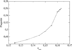
Figure 2: Average plaquettes for runs with three dynamical flavors at $\beta=5.3$.

For the determination of the critical value, $\kappa_{\mbox{\tiny crit}}$, the first method from Sec. 2 is adopted. Table 3 shows the average smallest and largest eigenvalues of $\tilde{Q}^{2}$. The eigenvalues have been computed every $100$ trajectories, and the errors have again been estimated using the Jackknife method.

$\mathbf{\kappa}$	$\mathbf{\lambda_{\mbox{\tiny\bf min}}}$	$\mathbf{\lambda_{\mbox{\tiny\bf max}}}$	$\mathbf{\lambda_{\mbox{\tiny\bf max}}/\lambda_{\mbox{\tiny\bf min}}}$
$0.125$	$0.2055(6)$	$1.7034(3)$	$8.288(12)$
$0.135$	$0.1331(7)$	$1.8426(5)$	$13.844(49)$
$0.145$	$0.07298(52)$	$1.9997(5)$	$27.40(19)$
$0.150$	$0.04539(76)$	$2.0836(10)$	$45.91(73)$
$0.155$	$0.02251(58)$	$2.1678(5)$	$96.3\pm 2.3$
$0.160$	$0.00764(65)$	$2.2367(18)$	$292.9\pm 25.1$
$0.161$	$0.00894(75)$	$2.2545(6)$	$252.2\pm 4.6$
$0.162$	$0.00633(51)$	$2.2722(8)$	$359.2\pm 28.9$
$0.163$	$0.00885(66)$	$2.2908(12)$	$258.9\pm 19.3$

Table 3: Average extremal eigenvalues and condition numbers for runs with three dynamical flavors at $\beta=5.3$.

Figure 3 shows the resulting plot of $1/\kappa$ vs. the inverse condition number $\lambda_{\mbox{\tiny min}}/\lambda_{\mbox{\tiny max}}$ of $\tilde{Q}^{2}$.

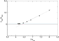
Figure 3: Inverse condition number of $\tilde{Q}^{2}$ vs. $1/\kappa$ for three dynamical fermions at $\beta=5.3$.

The straight line is a fit to the points between $1/\kappa=6.452$ and $1/\kappa=8.0$ which is parameterized by

$$\lambda_{\mbox{\tiny min}}/\lambda_{\mbox{\tiny max}}=-0.4610(13)+0.07252(17)/\kappa\,.$$ (7)

From the point where $\lambda_{\mbox{\tiny max}}/\lambda_{\mbox{\tiny min}}$ diverges (and thus $\kappa\rightarrow\kappa_{\mbox{\tiny crit}}$) one finds

$$\kappa_{\mbox{\tiny crit}}=0.1573(4)\,.$$ (8)

This method requires little effort and has a rather small error on the critical value of $\kappa$. However, the estimate (8) still contains a systematic uncertainty due to the fact that one is still rather far from the chiral regime.

2 The Case $\beta=5.2$

The point considered in the previous section already showed signs of the shielding transition as the condition number of $\tilde{Q}^{2}$ still was below $100$. Hence, this value of $\beta$ does not allow to probe the chiral regime further if one is limited to such small lattices. It can, however, be considered as a working point for future studies on larger lattices. As a different starting point, the focus will now be placed on the point $\beta=5.2$ with lattice sizes of $\Omega=16\times 8^{3}$ instead. This lattice size might already allow for a measurement of the ratio $m_{\pi}/m_{\rho}$ for degenerate sea and valence quark masses and hence for an independent estimate of the chiral transition. Again, the finite-temperature phase of QCD has to be avoided.

For the actual simulation, again several values for $\kappa_{\mbox{\tiny sea}}$ have been chosen. The polynomial parameters are given in Tab. 4. The runs have been performed on the ALiCE-cluster with a partition of eight nodes for each run.

$\mathbf{n_{1}}$	$\mathbf{n_{2}}$	$\mathbf{n_{3}}$	$\mathbf{[\epsilon,\lambda]}$	Updates/Configuration
$24$	$300$	$450$	$[7.5\times 10^{-4},3]$	$1$ boson HB, $5$ boson OR,
				$2$ gauge Metropolis, $1$ noisy corr.
Volume: $\Omega=16\times 8^{3}$

Table 4: Algorithmic parameters for each configuration for the runs at $\beta=5.2$ with $N_{f}=3$.

In general, one can expect that the polynomial orders and intervals are chosen somewhat conservatively and one could achieve some gain by adapting them manually with respect to the spectrum of $\tilde{Q}^{2}$ obtained during the production. Despite the lengths of the runs, it might still make sense to improve the statistics further.

The working points chosen are listed in Tab. 5 together with the acceptance rate of the noisy correction step, the number of performed trajectories, and the average plaquette with the error determined from the Jackknife method. From the Jackknife estimate, the plaquette autocorrelation time has been determined. Finally the correction factor with its standard deviation is shown.

$\mathbf{\kappa_{\mbox{\tiny sea}}}$	Number of confs.	$\mathbf{P_{\mbox{\tiny\bf acc}}}$	Plaquette	$\mathbf{\tau_{\mbox{\tiny\bf int}}}$	Rew. factor
$0.156$	$16700$	$30.30\%$	$0.4794(9)$	$1135$	$1.0000(1)$
$0.158$	$19980$	$27.27\%$	$0.4860(11)$	$1359$	$1.0001(2)$
$0.160$	$20100$	$30.35\%$	$0.4923(4)$	$359$	$1.0001(2)$
$0.162$	$34710$	$24.62\%$	$0.5105(?)$	-	$1.0000(2)$
$0.163$	$9200$	$17.92\%$	$0.5356(8)$	$735$	$0.9998(6)$
$0.164$	$24490$	$18.99\%$	$0.5443(6)$	$1062$	$0.97(10)$
$0.165$	$11510$	$25.54\%$	$0.5478(3)$	$286$	$1.0000(2)$
$0.166$	$10900$	$26.51\%$	$0.5508(2)$	$116$	$1.0000(2)$

Table 5: Simulation runs using three dynamical fermion flavors at $\beta=5.2$.

The plaquette for the run at $\kappa_{\mbox{\tiny sea}}=0.162$ showed a fluctuation between two different points and is plotted in Fig. 4. This is an indication that the shielding transition takes place around this point. Since the series is too short to make any statement about this fluctuation, the standard error is not shown here.

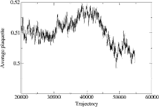
Figure 4: Plaquette history of the run at $\beta=5.2$ and $\kappa_{\mbox{\tiny sea}}=0.162$ with $N_{f}=3$.

In the cases $\kappa_{\mbox{\tiny sea}}=0.156$ and $\kappa_{\mbox{\tiny sea}}=0.158$ the autocorrelation time appears to be very large. Hence, the statistics are still comparatively small at these working points.

The magnitude of the reweighting factors in Tab. 5 confirms the expectation that the polynomial has been chosen very conservatively in most cases. However, the run at $\kappa_{\mbox{\tiny sea}}=0.164$ has a large fluctuation in the reweighting factor, which means that the smallest eigenvalue went off the polynomial interval. The precise situation is displayed in Fig. 5 after the thermalization phase has been subtracted. If this run was to be continued, one may consider to use polynomials with a smaller value of the lower limit for the approximation interval. The properly reweighted values may still be used for this analysis, but the statistics may be worse for this case. For the other simulation runs, one can conclude that reweighting can safely be disregarded.

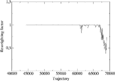
Figure 5: History of reweighting factors for the run at $\beta=5.2$ and $\kappa_{\mbox{\tiny sea}}=0.164$ with $N_{f}=3$.

Figure 6 shows the resulting values of the average plaquette as a function of the hopping parameter $\kappa_{\mbox{\tiny sea}}$. This plot corroborates that the shielding transition is located around $\kappa_{\mbox{\tiny sea}}=0.162$.

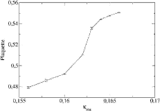
Figure 6: Average plaquettes for runs with three dynamical flavors at $\beta=5.2$.

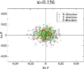
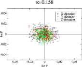
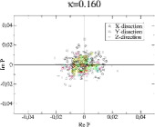
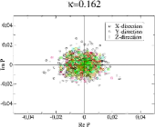
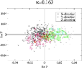
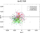
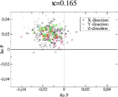
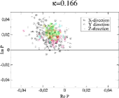
Figure 7: Polyakov loops along the shortest length, $L_{s}=8$, for the simulation of three dynamical fermion flavors at $\beta=5.2$.

Locating the Shielding Transition

As a first guideline of where the crossover to the shielded phase takes place, the plaquette fluctuation in Fig. 4 and the jump in the average plaquette in Fig. 6 have been considered. To gain further insight one can investigate the behavior of the average Polyakov loop, see Sec. 1. However, in this case it should now be measured in spatial (i.e. $x$, $y$, and $z$) direction since the $t$-direction is now the longest. The Polyakov line in that direction can be expected to show no sign of the finite-temperature phase.

The Polyakov loops have been measured every $100$ trajectories. The resulting values are shown in Fig. 7. Starting with $\kappa_{\mbox{\tiny sea}}=0.163$, one clearly sees a clustering in one of the three sectors. It is surprising that despite the rather long runs, in each case the values are clustered in only one sector. This indicates that the samples are not decorrelated with respect to this observable. At $\kappa_{\mbox{\tiny sea}}=0.162$ the shielding transition is not yet apparent in the Polyakov loop. However, when considering the previous indications, it appears safer to disregard the latter run from the following analysis.

Computing $m_{\pi}/m_{\rho}$

The details for the measurement of hadronic masses have been given in Sec. 3. As has been discussed above, only the points $\kappa_{\mbox{\tiny sea}}\leq 0.160$ should be considered for this analysis. The reweighting factor has been included, although it had no practical influence in these productions.

In the run with $\kappa=0.156$ the correlation functions for the (non-singlet) pseudoscalar and the vector mesons are visualized in Figs. 8 and 9. These functions have already been symmetrized, i.e. the plot shows (cf. Eq. (35))

$$\Gamma_{\mbox{\tiny$\pi,\rho$}}^{\mbox{\tiny sym}}(t)=\frac{1}{2}\left(\Gamma_{\mbox{\tiny$\pi,\rho$}}(t)+\Gamma_{\mbox{\tiny$\pi,\rho$}}(L_{0}-t)\right)\,,$$

with $L_{0}$ being the lattice extension in $t$-direction.

These functions should follow the behavior given in Eq. (36). However, for small values of $t$, one expects the results to be too large (due to the contamination with higher modes, cf. Sec. 3), while for larger values of $t$, larger autocorrelations of the greater lengths may result in worse statistics.

To obtain an estimate for the autocorrelation time of these masses, the Jackknife method has again been employed. The case which is considered in detail is the run at $\kappa=0.156$. Figures 10 and 11 show the variances of the masses for a fit interval from timeslice $t=5$ to timeslice $t=7$.

Quantity	Expect. value	Variance $\mathbf{\sigma^{2}}$	$\mathbf{\sigma^{2}(B=1)}$	$\tau_{\mbox{\tiny int}}$
$(am_{\pi})$	$1.374(12)$	$1.436\times 10^{-3}$	$1.163\times 10^{-5}$	$6.18$
$(am_{\rho})$	$1.440(13)$	$1.803\times 10^{-3}$	$1.804\times 10^{-5}$	$5.00$

Table 6: Jackknife variances together with the corresponding variances for bin size $B=1$ for the simulation run at $\beta=5.2$ and $\kappa=0.156$. From there, an estimate for the integrated autocorrelation time is obtained.

The resulting values are given in Tab. 6 together with the variance estimate for bin size $B=1$. By exploiting Eq. (30), one can as usual obtain an estimate for the autocorrelation time of the quantity under consideration.

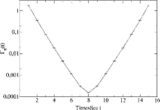
Figure 8: Symmetrized correlation function for the pseudoscalar meson with three dynamical fermions at $\beta=5.2$ and $\kappa=0.156$.

Since the correlators have been computed every $100$ trajectories, the results imply that the $\pi$- and $\rho$-mesons have autocorrelation times of $\tau_{\mbox{\tiny int}}^{\pi}\approx 618$ and $\tau_{\mbox{\tiny int}}^{\rho}\approx 500$ trajectories, respectively. These numbers are slightly better than what the plaquette has indicated, albeit still large. A source of this problem is the choice of the first polynomial. If the GMRES method had been used instead, one might have achieved a faster decorrelation by reducing the polynomial order, $n_{1}$, see Sec. 2 and also Sec. 3.

Figure 12 shows the resulting values for masses in lattice units. The lower limit of the fit is given by the timeslice $t$, while for the upper limit, always the next-to-last limit has been used, i.e. $L_{0}^{\mbox{\tiny max}}=7$. The error is again taken to be the standard error, which has been computed using the Jackknife procedure as above in Tab. 6. The method follows the results discussed in [150, 148, 227, 9].

The plateaus in Fig. 12 are reached at $t=5$. Therefore, the values obtained at this point will be used in the following. Table 7 summarizes all results together with the autocorrelation times determined using the Jackknife scheme. In the case $\kappa=0.160$, no plateau could have been identified and the results are compatible with an integrated autocorrelation time below $100$ trajectories.

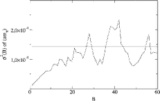
Figure 10: Jackknife variances for different bin sizes for the mass of the pseudoscalar meson with three dynamical fermions at $\beta=5.2$ and $\kappa=0.156$. The mass is obtained from a fit to an interval $[t_{\mbox{\tiny min}}=5,t_{\mbox{\tiny max}}=7]$.

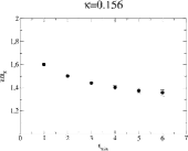
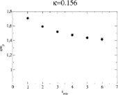
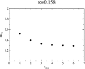
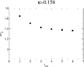
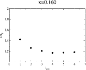
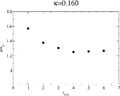
Figure 12: Meson masses in lattice units as a function of the fitting interval for three dynamical fermions at $\beta=5.2\,$.

$\mathbf{\kappa}$	$\mathbf{(am_{\pi})}$	$\mathbf{(am_{\rho})}$	$\mathbf{m_{\pi}/m_{\rho}}$	$\mathbf{a}$	$\mathbf{\tau_{\mbox{\tiny int}}^{\pi}}$	$\mathbf{\tau_{\mbox{\tiny int}}^{\rho}}$
$0.156$	$1.374(12)$	$1.440(13)$	$0.954(18)$	$0.368(3)$	$618$	$508$
$0.158$	$1.298(15)$	$1.377(16)$	$0.943(16)$	$0.352(4)$	$620$	$565$
$0.160$	$1.1767(52)$	$1.2604(84)$	$0.9336(75)$	$0.323(2)$	$<100$	$<100$

Table 7: Masses and their autocorrelation times for the determination of the ratio $m_{\pi}/m_{\rho}$ for three dynamical fermions at $\beta=5.2$.

Locating the Critical Point

To locate the critical point, again the smallest and largest eigenvalues have been computed and the condition numbers have been determined for the runs at $\beta=5.2$. The eigenvalues have been computed every $100$ trajectories. Table 8 summarizes the findings.

$\mathbf{\kappa}$	$\mathbf{\lambda_{\mbox{\tiny\bf min}}}$	$\mathbf{\lambda_{\mbox{\tiny\bf max}}}$	$\mathbf{\lambda_{\mbox{\tiny\bf max}}/\lambda_{\mbox{\tiny\bf min}}}$
$0.156$	$0.0330(6)$	$2.2137(5)$	$67.1\pm 1.1$
$0.158$	$0.0249(3)$	$2.2503(9)$	$90.4\pm 3.2$
$0.160$	$0.0178(2)$	$2.2879(5)$	$128.5\pm 3.3$

Table 8: Average extremal eigenvalues and condition numbers for runs with three dynamical flavors at $\beta=5.2$.

The inverse condition number is plotted vs. the inverse quark mass in Fig. 13.

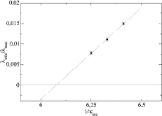
Figure 13: Inverse condition number of $\tilde{Q}^{2}$ vs. $1/\kappa$ for three dynamical fermions at $\beta=5.2$.

The fit to all three data points yields

$$\lambda_{\mbox{\tiny min}}/\lambda_{\mbox{\tiny max}}=-0.272(18)+0.0448(28)/\kappa\,.$$ (9)

The zero of the line gives

$$\kappa_{\mbox{\tiny crit}}=0.1645(29)\,.$$ (10)

Finally, the fitting function from Eq. (6) is applied to the situation at hand with the pion masses given by Tab. 7. In Fig. 14 the inverse value of the quark mass, $1/\kappa$, is plotted versus the square of the pion mass, $(am_{\pi})^{2}$. In addition, the rho mass, $(am_{\rho})$, is also included in this plot. The former is visualized as circles, while the latter is pictured by squares. The shielding transition is shown as a magenta bar.

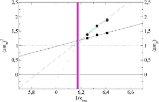
Figure 14: Square of the pion mass, $(am_{\pi})^{2}$, (black circles) and the rho mass, $(am_{\rho})$, (black squares) for $\beta=5.2$ with $N_{f}=3$.

The linear fit to $(am_{\pi})^{2}$ is given by the solid green line in Fig. 14. The curve is parameterized by

$$(am_{\pi})^{2}=-(19.60\pm 1.94)+(3.359\pm 0.309)/\kappa\,.$$ (11)

The critical value of $\kappa_{\mbox{\tiny crit}}$ is then found to be

$$\kappa_{\mbox{\tiny crit}}=0.1713(67)\,.$$ (12)

The result from Eq. (12) agrees within the errors with the previous result from Eq. (10).

Furthermore, a quadratic curve has been drawn through the values for $(am_{\pi})^{2}$, given by the green dashed line. It is parameterized by

$$(am_{\pi})^{2}=-340.81+105.06/\kappa-8.05/\kappa^{2}\,.$$ (13)

When using this curve, the resulting value for $\kappa_{\mbox{\tiny crit}}$ is found to be

$$\kappa_{\mbox{\tiny crit}}=0.1659\,.$$ (14)

The linear fit to $(am_{\rho})$ is given by the blue line in Fig. 14. The curve is parameterized by

$$(am_{\rho})=-(5.91\pm 0.60)+(1.147\pm 0.095)/\kappa\,.$$ (15)

Obviously, it is not possible to reach values of $\xi_{\pi}>1$ before the shielding transition sets in on the current lattice size, cf. Sec. 2. Therefore, the linear extrapolation in Eq. (11) may be biased with an uncontrolled systematic uncertainty. To estimate this effect, one may compare the resulting critical point, Eq. (12), with the result obtained from the quadratic fit, Eq. (14). This uncertainty makes further investigations closer to the chiral point necessary and consequently implies the need to go to larger lattices.

Prospects for Future Simulations

Up to this point, one could only achieve ratios of $m_{\pi}/m_{\rho}>0.9$ with $\xi_{\pi}<1$. When going to larger lattices, the shielding transition will set in at larger values of $\kappa_{\mbox{\tiny sea}}$, allowing to probe lighter quark masses.

A procedure for continuing along this line of research consists of going to $\Omega=24\times 12^{3}$ lattices, starting from $\kappa_{\mbox{\tiny sea}}\geq 0.160$ until the shielding transition for the new lattice sets in. In light of the fact that the shielding transition in Fig. 14 is located shortly before one arrives at $\xi_{\pi}\geq 1$, a lattice size of $L_{s}=12$ might already be sufficiently large to obtain a set of data points all fulfilling the requirement $\xi_{\pi}>1$. In such a situation, one could obtain an extrapolation to the chiral point, $\kappa_{\mbox{\tiny crit}}$, with reduced systematic uncertainty.

Bare parameters			Physical parameters
$\mathbf{N_{f}^{\mbox{\tiny sea}}}$	$\mathbf{\beta^{\mbox{\tiny spec}}}$	$\mathbf{\kappa}^{\mbox{\tiny spec}}$	$\mathbf{(am_{\pi})}$	$\mathbf{(am_{\rho})}$	$\mathbf{m_{\pi}/m_{\rho}}$	$\mathbf{a}$/fm
$3$	$5.2$	$0.169(23)$	$0.5$	$0.882$	$0.567$	$0.226$

Table 9: The suggested working point for future spectroscopic studies on lattices with $\Omega=32\times 16^{3}$ and beyond.

With the available information we can, however, still try to locate a working point at this particular value of $\beta$ in the $\beta$-$\kappa$-plane with properties similar to the point chosen for the SESAM-project [133].

This working point will now be denoted $\left(\beta^{\mbox{\tiny spec}},\kappa^{\mbox{\tiny spec}}\right)$. With the uncertainties discussed above in mind, we imposes the following constraints:

$$z \equiv \xi_{\pi}/L<1/4\,,$$

$$\xi_{\pi} \geq 2\,.$$ (16)

The actual parameters can be identified from the extrapolations Eqs. (11) and (15). First, from setting $\xi_{\pi}=2$, we obtain

$$\kappa^{\mbox{\tiny spec}}=0.169(23)\,.$$ (17)

From the requirement (2) that the value of the finite-size parameter should be $z<1/4$, one finds, in accordance with the SESAM-data from [227], that one has to go to lattices with at least $L_{s}=16$ if one wants to explore this region in parameter space.

The parameters for this working point are summarized in Tab. 9. The estimated values for $(am_{\rho})$, $m_{\pi}/m_{\rho}$, and $a$ have been computed from the fit (15). The total physical lattice size $L_{s}$ would then be $L_{s}=3.616\;\mbox{fm}$. A possible criticism against this working point might be that this lattice spacing is rather coarse. To actually increase the resolution, one would need to go to higher values of $\beta$, thus moving closer to the continuum limit.

Finally, the question arises how large the total effort might be for such a project. For the case of quadratically optimized polynomials, it has been argued in [218], that the required increase in $n_{1}$ when going from $N_{f}=2$ to $N_{f}=3$ is only of the order of about $30\%$. Reference [240] confirms this finding by stating that going from $N_{f}=1/2$ to $N_{f}=3$ will only increase $n_{1}$ by about $50\%$. Taking — as a very conservative estimate — the latter number to be applicable also to the simulations performed for $N_{f}=2$ in chapter 4, we find by applying Eq. (12) that the total cost for an independent configuration (with respect to the plaquette) is about

$$E_{\mbox{\tiny indep}}\simeq(1.5)^{2}\cdot(1075360\pm 72160)\approx(2420000\pm 162000)\,,$$ (18)

when considering the lightest quark mass, where $m_{\pi}/m_{\rho}=0.6695$. Hence, this estimate marks the upper limit for the effort required in a simulation similar to the SESAM-project, provided one decides to take recourse to an MB algorithm. The total cost quoted in Eq. (18) is still smaller than the corresponding cost for the HMC run with $N_{f}=2$. Therefore, one can expect the simulations at the lighter quark masses to be even cheaper than they were in the case of the SESAM-project.

4 Summary and Outlook

A first step towards the simulation of QCD with three degenerate dynamical quark flavors has been taken. The TSMB algorithm been applied successfully to this physically interesting situation. The simulations have yielded first results for the shielding transitions on the current lattice size with $L_{s}=8$ and the critical points at two values of $\beta$. It has become clear that there is no window for doing spectroscopy at the parameters chosen.

Prospects for future simulations have been given and a potential working point has been estimated, although with large systematic uncertainty. It has been argued that a study with physical masses similar to the SESAM-project is feasible today and might even cost slightly less than the HMC-based program.

In an ongoing research project, such type of simulations will be performed on larger lattices and closer to the chiral limit. For the current status of the comprehensive project see [240].

A potential obstacle for future simulations with three dynamical fermion flavors may still be posed by the fermionic sign problem. As has been noted in Sec. 4, the fermionic determinant will change its sign if an odd number of real eigenvalues becomes negative. The polynomial approximations in Sec. 1, however, are applied to the square of the Hermitian Wilson matrix. Hence, they will always yield a positive sign. Consequently, the sign would have to be included into the measurement of observables which may eventually spoil the statistical quality of the sample. A similar problem is known to occur in the simulation of gauge theories with a non-zero chemical potential, see [190].

Such a problem does not show up for an even number of degenerate fermion flavors since in that case squaring the Wilson matrix will always yield a positive sign. The only known way to overcome this obstacle directly in a sampling process has been found for some quantum spin systems (cf. Sec. 3). It is yet unclear, if any quantum spin system similar to gauge theories with dynamical fermion flavors can be simulated efficiently in such a manner. However, as has already pointed out in Sec. 3, it may be that this sign problem is not significant in actual simulations of QCD.

Chapter 6 Summary and Outlook

A foresighted strategy can help to find

a winning move in a superior position.

In this thesis algorithms for the simulation of quantum field theories with dynamical fermionic degrees of freedom have been presented. Special emphasis has been put on a new class of algorithms, namely the multiboson algorithms which represent the fermionic determinant by a number of boson fields. They allow for the implementation of local updating algorithms, which are known to be superior to global schemes applicable to gauge theories so far.

A particular variant of these algorithms, the TSMB method, has been implemented on several machines. This scheme relies on the computation of powers of matrices using static polynomials. The parameters which fix a given polynomial are the order and the interval of the approximation. Beyond that, it has turned out that the choice of the updating scheme is important.

The optimal settings for these parameters have been determined and the sensitivity of the system to sub-optimal tuning has been analyzed. Furthermore, different updating schemes have been examined with respect to their efficiency and recommendations for the implementations of multiboson algorithms in general have been given.

Due to the complexity of MB schemes, however, there is still room for improvement. MB algorithms remain open for refinements in the future, but can already be used for large-scale simulations today.

Major emphasis has been put on how multiboson algorithms compare to their competitors in the field of dynamical fermion simulations. We have shown that, with sufficient tuning, MB algorithms appear to be superior to the HMC algorithm in the case of light quark masses. We would expect that further improvements in MB algorithms will be found with growing experience in future simulations. This might help the MB scheme to replace the HMC method as the standard algorithm in Lattice QCD.

The final part of this thesis has considered the application of the TSMB algorithm to the case of three dynamical fermionic flavors, a situation which is of great importance for realistic simulations of QCD. Based on this experience, a proposal for future simulations has been formulated. In fact, one can be optimistic to perform a project similar to SESAM at reasonable cost. A working point for such type of simulations on $\Omega=32\times 16^{3}$ lattices has been estimated, where semi-realistic simulations with good statistics should be run. This would provide an assessment of an operating window in the $N_{f}=3$ scenario.

In conclusion, we find that multiboson algorithms provide a great leap forward in the simulation of Lattice QCD and give us the means to perform simulations in realistic scenarios.

Chapter 7 Notations and Conventions

Unless otherwise explicitly stated, natural units have been adopted throughout this thesis by setting

$$\hbar=c=k_{B}=1\,.$$ (1)

The four-dimensional Minkowski-space is denoted by $\mathbb{M}^{4}$ and has the canonical flat-space metric

$$g_{\mu\nu}=\left(\begin{array}[]{*{4}{p{0.35cm}}}1&0&0&0\\ 0&-1&0&0\\ 0&0&-1&0\\ 0&0&0&-1\end{array}\right)\,.$$ (2)

The Wick rotation

$$x\mapsto x^{\prime}:x^{\prime}=\left(x^{\prime}_{0},\mathbf{x}^{\prime}\right)=\left(-\mbox{i}x_{0},\mathbf{x}\right)$$ (14)

transforms vectors from Minkowski-space to the Euclidean space $\mathbb{R}^{4}$ with the metric given by the Kronecker symbol $\delta_{\mu\nu}$:

$$\delta_{\mu\nu}=\left\{\begin{array}[]{l}1,\qquad\mbox{for }\mu=\nu,\\ 0,\qquad\mbox{for }\mu\neq\nu.\end{array}\right.$$ (3)

The discrete space of the lattice theory is denoted by $\mathbb{Z}^{4}$. Vectors in space are always denoted by $x$. Unit vectors are only used in $\mathbb{Z}^{4}$, where they are written as $\hat{\mu}$ with $\mu=0,\dots,3$. If the lattice volume is finite, the lengths $L_{\mu}$ in direction $\mu$ are also denoted by $L_{t}=L_{0}$ and $L_{s}=L_{1}=L_{2}=L_{3}$, where $L_{t}$ is the lattice size in “time” and $L_{s}$ in “space” direction. The total volume is denoted by $\Omega=\prod_{\mu}L_{\mu}=L_{t}\times L_{s}^{3}$ and the corresponding space is $\mathbb{Z}^{4}_{\Omega}$. For different lengths $L_{1}$, $L_{2}$, and $L_{3}$, the notation $\Omega=L_{0}\times L_{1}\times L_{2}\times L_{3}$ will be used. For a bosonic field, $\phi(x)\in\mathbb{Z}^{4}_{\Omega}$, periodic boundary conditions are imposed:

$$\phi\left(x+\hat{\mu}L_{\mu}\right)=\phi\left(x\right)\,.$$

Here $x+\hat{\mu}$ denotes the point adjacent to $x$ in direction $\mu$.

The totally antisymmetric $4$-tensor $\epsilon^{\mu\nu\rho\sigma}$ obeys

$$\epsilon^{\left[\mu\nu\rho\sigma\right]}=\left\{\begin{array}[]{ll}-1,\qquad\mbox{for $\left[\mu\nu\rho\sigma\right]$ being an odd permutation of $0123$},\\ +1,\qquad\mbox{for $\left[\mu\nu\rho\sigma\right]$ being an even permutation of $0123$},\\ \phantom{+}0,\qquad\mbox{otherwise}.\end{array}\right.$$

The commutator of two objects $A,B$ for which multiplication and addition are defined is denoted by

$$\left[A,B\right]=A\cdot B-B\cdot A\,.$$

The anti-commutator is denoted by

$$\left\{A,B\right\}=A\cdot B+B\cdot A\,.$$

Appendix 7.A Dirac Matrices

The Dirac matrices $\tilde{\gamma}_{\mu}$, $\mu=0,\dots,3$, in Minkowski space are defined by

$$\left\{\tilde{\gamma}_{\mu},\tilde{\gamma}_{\nu}\right\}=2g_{\mu\nu}\,.$$ (4)

The matrix $\tilde{\gamma}_{5}$ is defined by

$$\tilde{\gamma}_{5}=\tilde{\gamma}^{5}=\mbox{i}\tilde{\gamma}_{0}\tilde{\gamma}_{1}\tilde{\gamma}_{2}\tilde{\gamma}_{3}=-\frac{\mbox{i}}{4!}\epsilon_{\mu\nu\rho\sigma}\tilde{\gamma}^{\mu}\tilde{\gamma}^{\nu}\tilde{\gamma}^{\rho}\tilde{\gamma}^{\sigma}=\tilde{\gamma}_{5}^{\dagger}\,.$$ (5)

It satisfies $\tilde{\gamma}_{5}^{2}=\mathbf{1}$, and $\{\tilde{\gamma}_{5},\tilde{\gamma}_{\mu}\}=0$. The chirality projectors $P_{R,L}$ are given by

$$P_{R,L}=\frac{1}{2}\left(1\pm\tilde{\gamma}_{5}\right)\,.$$ (6)

When performing the Wick rotation, the Euclidean Dirac matrices are given by

$$\left\{\gamma_{\mu},\gamma_{\nu}\right\}=2\delta_{\mu\nu}\,.$$ (7)

They are related via [24]

$$\gamma_{1,2,3}=-\mbox{i}\tilde{\gamma}_{1,2,3},\qquad\gamma_{0}=-\tilde{\gamma}_{0}\,.$$

The Euclidean $\gamma_{5}$-matrix is given by $\gamma_{5}=\gamma_{1}\gamma_{2}\gamma_{3}\gamma_{0}$.

The matrices with smallest dimension satisfying (4) are $4\times 4$ matrices [11]. The representation of the $\gamma_{\mu}$-matrices employed in this thesis has been chosen to be the “chiral” one, where the Minkowski-space matrices are given by

$$\begin{array}[]{ll}\tilde{\gamma}_{0}=\left(\matrix{0&0&-1&0\\ 0&0&0&-1\\ -1&0&0&0\\ 0&-1&0&0\\ }\right),&\tilde{\gamma_{1}}=\left(\matrix{0&0&0&1\\ 0&0&1&0\\ 0&-1&0&0\\ -1&0&0&0\\ }\right),\\ &\\ \tilde{\gamma}_{2}=\left(\matrix{0&0&0&-\mbox{i}\\ 0&0&\mbox{i}&0\\ 0&\mbox{i}&0&0\\ -\mbox{i}&0&0&0\\ }\right),&\tilde{\gamma}_{3}=\left(\matrix{0&0&1&0\\ 0&0&0&-1\\ 1&0&0&0\\ 0&-1&0&0\\ }\right),\\ &\end{array}$$ (12)

$$\begin{array}[]{l}\tilde{\gamma}_{5}=\left(\matrix{1&0&0&0\\ 0&1&0&0\\ 0&0&-1&0\\ 0&0&0&-1\\ }\right)\,.\end{array}$$ (14)

The Euclidean $\gamma_{\mu}$ matrices are then given by

$$\begin{array}[]{ll}\gamma_{0}=\left(\matrix{0&0&1&0\\ 0&0&0&1\\ 1&0&0&0\\ 0&1&0&0\\ }\right),&\gamma_{1}=\left(\matrix{0&0&0&-\mbox{i}\\ 0&0&-\mbox{i}&0\\ 0&\mbox{i}&0&0\\ \mbox{i}&0&0&0\\ }\right),\\ &\\ \gamma_{2}=\left(\matrix{0&0&0&-1\\ 0&0&1&0\\ 0&1&0&0\\ -1&0&0&0\\ }\right),&\gamma_{3}=\left(\matrix{0&0&-\mbox{i}&0\\ 0&0&0&\mbox{i}\\ \mbox{i}&0&0&0\\ 0&-\mbox{i}&0&0\\ }\right),\\ &\end{array}$$ (19)

$$\begin{array}[]{l}\gamma_{5}=\left(\matrix{1&0&0&0\\ 0&1&0&0\\ 0&0&-1&0\\ 0&0&0&-1\\ }\right)\,.\end{array}$$ (21)

The contraction of a four-vector $A^{\mu}$ with the Dirac matrices is denoted by

$$/\!\!\!\!A=\sum_{\mu=0}^{3}A^{\mu}\gamma_{\mu}.$$ (22)

Chapter 8 Groups and Algebras

One of the central concepts of particle physics is the notion of symmetry groups. All particles transform according to a symmetry of space-time and the symmetries of the Lagrangian. In the relativistic case this will mean that they transform as representations of the proper orthochroneous Poincaré-group, see below.

Appendix 8.A Groups and Representations

A group is a pair $\left(G,\cdot\right)$ of a set $G$ and a relation $\cdot$, satisfying the following axioms

1. The operation $\cdot$ is associative, i.e. $\forall\ x,y,z\in G$ holds $\left(x\cdot y\right)\cdot z=x\cdot\left(y\cdot z\right)$.

2. There is a unit element $e\in G$ satisfying: $\forall\ x\in G$ holds $x\cdot e=e\cdot x=x$.

3. For every $x\in G\,\;\exists\ x^{-1}\in G$ such that $x\cdot x^{-1}=x^{-1}\cdot x=e$.

The group is called Abelian (or commutative) if additionally $\left[x,y\right]=x\cdot y-y\cdot x,\forall\ x,y\in G$ holds. It follows immediately that the unit element is uniquely determined. Furthermore it follows that the inverse element $x^{-1}$ for each $x$ is unique.

A representation $\mathscr{R}(G)$ of the group $G$ is a group homomorphism from $G$ to the group of vector space endomorphisms of a representation space $V$, $\mathscr{R}(G):g\mapsto M(g)$, $g\in G$ and $M(g)\in V$ with the following properties:

1. $M(g)\cdot M(h)=M(g\cdot h)$, i.e. the representation respects the group multiplication of $G$,

2. $M(\mathbf{1})=\mathbf{1}$, i.e. the image of the unit element in $G$ is the identity in $V$,

3. $M(g^{-1})=M^{-1}(g)$, i.e. the image of the inverse element is the inverse of the group element.

A representation is called irreducible if it can not be written as the direct sum of other representations. Thus, there are no invariant subspaces under the action of the $M(g)$ for all $g\in G$. In the following, a matrix in $V$ (with an appropriate basis) with the above properties will be called a representation of $G$.

Particles, as observed in nature, should certainly be independent of the way we choose our coordinate system, i.e. how we choose the basis for the representation space $V$ (this requirement parallels the requirement of the theories to be coordinate invariant). Thus, they should always be classified by irreducible representations of a group. These irreducible representations also go under the name multiplet.

Of particular interest to physics are the Lie groups, see for a textbook [244]. A Lie group is a group for which the multiplication law and taking the inverse are smooth functions. Thus, the group space must be a manifold and one can form the tangent space on any point in the group. The tangent space on the unit element is called the Lie algebra of the group. A basis of the Lie algebra is called the set of generators of the group. Accordingly, an element $a$ of a Lie group $a\in L$ can be written in terms of the generators $\{g_{i}\}$, $i=1,\dots,N$ as:

$$a=\exp\left[\sum_{i=1}^{N}\omega_{i}g_{i}\right]\,,$$ (1)

where the element $a$ is parameterized using the $\{\omega_{i}\}$ as coordinates. The dimension of a Lie group is thus the dimension of the underlying manifold of the group space. A Lie algebra can be specified by the structure constants $f_{abc}$, which are defined via

$$\left[g_{a},g_{b}\right]=f_{abc}g_{c}\,.$$ (2)

For the integration over the group space, there exists a unique measure on $G$ called the Haar measure, $dU$, which obeys:

1. Consider a function $f:G\rightarrow\mathbb{C}$. Then $dU$ obeys for all $V\in G$

   $$\int_{G}\;dUf(U)=\int_{G}\;dUf(V\cdot U)=\int_{G}\;dUf(U\cdot V)\,.$$

2. The integral is normalized, i.e. $\int_{G}dU=1$.

It satisfies

$$\int_{G}dU\;f(U)=\int_{G}dU\;f(U^{-1})\,.$$

The rank of a group is the number of generators that simultaneously commute among themselves. It is thus the maximum number of generators which can simultaneously be diagonalized.

A Lie algebra is called semisimple, if for some $z\in G$, there are $x,y\in G$ with $z=\left[x,y\right]$. It can be shown, that for any compact Lie group, the algebra can always be written as the direct sum of a semisimple Lie algebra and an Abelian one. The semisimple Lie algebras can be decomposed into a set of groups which are called simple. The latter cannot be written as sums of anything else. The simple groups fall into the following categories:

1. The algebra sl${}_{N}(\mathbb{C})$, the $N\times N$ complex matrices with vanishing trace. The compact real form of sl${}_{N}(\mathbb{C})$ is su$(N)$ and the corresponding Lie group is SU$(N)$, the $N\times N$ unitary matrices with unit determinant. In the case $N=1$, we speak of the group U$(1)$, which consists of the complex numbers on the unit circle.

2. The Lie algebra so${}_{2N+1}(\mathbb{C})$, the $(2N+1)\times(2N+1)$ skew-symmetric complex matrices with vanishing trace. The compact real form is so_N, and the Lie group generated is SO$(N)$, the $N\times N$ real, orthogonal matrices with determinant one. They form the rotation group in $N$-dimensional Euclidean space. The rotation group in Minkowski space whose metric changes sign on the diagonal is usually denoted with SO$(3,1)$, but still belongs to this category.

3. The Lie algebra sp${}_{N}(\mathbb{C})$, the $2N\times 2N$ complex matrices of the form

   $$\left(\begin{array}[]{cc}A&B\\ C&D\end{array}\right)\,,$$

   where $B$ and $C$ are symmetric, and $D$ is the negative transpose of $A$. The compact real form is sp$(N)$ and the Lie group is Sp$(N)$, which forms the group of $N\times N$ quaternionic matrices which preserve the inner product on the space $H^{N}$ of $N$-tuples of quaternions.

4. The Lie algebra so${}_{2N}(\mathbb{C})$, the $(2N)\times(2N)$ skew-symmetric complex matrices with vanishing trace. This is the even-dimensional analog of item 2 for even $N$. These groups are to be distinguished, since the physics in these cases may differ.

Apart from these classical algebras, there are also the groups $G_{4}$, $F_{2}$, $E_{6}$, $E_{7}$, and $E_{8}$. Some of these also have applications in physics, however, so far they are not considered to play any role for the purposes of this thesis.

The dimensions and ranks of the three important kinds of semi-simple groups in this thesis are shown in Tab. 1.

Group	Dimension	Rank
SO$(N)$, $N$ even	$\frac{1}{2}N(N-1)$	$N/2$
SO$(N)$, $N$ odd	$\frac{1}{2}N(N-1)$	$(N-1)/2$
SU$(N)$	$N^{2}-1$	$N-1$

Table 1: Most important semi-simple groups together with their dimension and rank. The table is taken from [245].

Appendix 8.B The U$(1)$ Group

The U$(1)$ group is a special case of the SU$(N)$ groups. It consists of the group of complex numbers on the unit circle. It is a commutative group since the complex numbers commute under multiplications.

Appendix 8.C The SU$(N)$ Groups

The SU$(N)$ groups consist of elements isomorphic to the $N\times N$ unitary matrices with unit determinant:

$$U\cdot U^{\dagger}=U^{\dagger}\cdot U=\mathbf{1},\qquad\mbox{det}\,U=1\,.$$ (3)

Obviously the matrices $U$ in (3) form already the fundamental representation of the SU$(N)$ group. In this thesis the groups SU$(2)$ and SU$(3)$ play a central role. The generators chosen for the specific realizations used in this thesis are listed in the following sections.

1 The SU$(2)$ Group

The standard choice for the generators of the SU$(2)$ group are the Pauli matrices:

$$\sigma_{1}=\left(\begin{array}[]{cc}0&1\\ 1&0\end{array}\right)\,,\quad\sigma_{2}=\left(\begin{array}[]{cc}0&-\mbox{i}\\ \mbox{i}&0\end{array}\right)\,,\quad\sigma_{3}=\left(\begin{array}[]{cc}1&0\\ 0&-1\end{array}\right)\,.$$ (4)

The peculiarity of SU$(2)$ is that these matrices together with the unit matrix,

$$\mathbf{1}=\left(\begin{array}[]{cc}1&0\\ 0&1\end{array}\right)\,,$$

form a basis of the complex $2\times 2$ matrices. The expansion coefficients form a hypersurface in the space of complex $2\times 2$ matrices, where the expansion coefficients are real. A consequence of this observation is that any sum of SU$(2)$ matrices is again proportional to an SU$(2)$ matrix. This property only exists in the case $N=2$. The proportionality factor can be computed by considering the inverse of a matrix $A$,

$$A=a_{0}+\mbox{i}\sum_{r=1}^{3}\sigma_{r}\mathbf{a}_{r}=\left(\begin{array}[]{cc}a_{0}+\mbox{i}a_{3}&a_{2}+\mbox{i}a1\\ -a_{2}+\mbox{i}a_{1}&a_{0}-\mbox{i}a_{3}\end{array}\right)\,.$$

Then the inverse is given by

$$A^{-1}=\frac{1}{\det A}A^{\dagger}=\frac{1}{\det A}\left(\begin{array}[]{cc}a_{0}-\mbox{i}a_{3}&-a_{2}-\mbox{i}a_{1}\\ a_{2}-\mbox{i}a_{1}&a_{0}+\mbox{i}a_{3}\end{array}\right)\,.$$

Consequently, the proportionality factor is given by $k=\sqrt{\det A}$, i.e. the matrix

$$B=A/\sqrt{\det A}$$ (5)

is an SU$(2)$ matrix.

From Tab. 1 it follows that the group has rank one, thus the representations correspond to the eigenvalues of a single operator. Usually, the eigenvalues of $\sigma_{3}$ are taken to classify the multiplets. SU$(2)$ is locally isomorphic to SO$(3)$ [15], which means that the algebras of the two groups are identical, although this does not hold for their global topology. To be specific, SU$(2)$ is the double-cover of SO$(3)$. While the latter is not simply connected, the former is.

2 The SU$(3)$ Group

In this thesis the Gell-Man matrices $\{\lambda_{i}\}$, $i=1,\dots,8$, as defined in [24] have been chosen as the generators of the SU$(3)$ group:

$$\begin{array}[]{lll}\lambda_{1}=\pmatrix{0&1&0\\ 1&0&0\\ 0&0&0\\ }\,,&\lambda_{2}=\pmatrix{0&-\mbox{i}&0\\ \mbox{i}&0&0\\ 0&0&0\\ }\,,&\lambda_{3}=\pmatrix{1&0&0\\ 0&-1&0\\ 0&0&0\\ }\,,\\ &\\ \lambda_{4}=\pmatrix{0&0&1\\ 0&0&0\\ 1&0&0\\ }\,,&\lambda_{5}=\pmatrix{0&0&-\mbox{i}\\ 0&0&0\\ \mbox{i}&0&0}\,,&\lambda_{6}=\pmatrix{0&0&0\\ 0&0&1\\ 0&1&0}\,,\\ &\\ \lambda_{7}=\pmatrix{0&0&0\\ 0&0&-\mbox{i}\\ 0&\mbox{i}&0},&\lx@intercol\lambda_{8}=\pmatrix{1/\sqrt{3}&0&0\\ 0&1/\sqrt{3}&0\\ 0&0&-2/\sqrt{3}}\,.\hfil\lx@intercol\end{array}$$ (11)

Appendix 8.D The Poincaré Group

The space-time manifold underlying the physical theories discussed in this thesis is given by the Minkowski-space. The metric is pseudo-Euclidean and can be transformed globally to the form

$$g_{\mu\nu}=\left(\begin{array}[]{*{4}{p{0.35cm}}}1&0&0&0\\ 0&-1&0&0\\ 0&0&-1&0\\ 0&0&0&-1\end{array}\right)\,.$$ (2)

An event is associated with a point in space-time, and the distance between two events is defined as

$$(x-y)^{2}=(x-y)^{\mu}(x-y)^{\nu}g_{\mu\nu}\,.$$ (12)

Here and in the following the Einstein summation convention that identical indices are to be summed over is understood. The quantity $a^{\mu}a^{\nu}g_{\mu\nu}\equiv a^{\mu}a_{\nu}$ is called the norm of $a^{\mu}$. This norm, however, is not positive definite. Depending on the sign of $a^{2}$, one defines the following classes of vectors:

Timelike region:

If $a^{2}=(x-y)^{2}>0$, the distance is called timelike. In such a case, the two events at $x^{\mu}$ and $y^{\mu}$ may have a causal influence on each other and there exists a unique Lorentz transformation which reduces the spatial components of $a^{\mu}$ to zero. However, there is no transformation which rotates the $a^{0}$ component to $0$.

Spacelike region:

If $a^{2}=(x-y)^{2}<0$, the distance is spacelike. In this case, two events at $x^{\mu}$ and $y^{\mu}$ cannot be causally related. This requirement is equivalent to the colloquial saying that “no information can travel faster than the speed of light”. There is a unique Lorentz transformation which rotates the $a^{0}$ component to $0$, but there is none which reduces the spatial components of $a^{\mu}$ to zero.

Likelight region:

If $a^{2}=(x-y)^{2}=0$, the distance between $x^{\mu}$ and $y^{\mu}$ is lightlike. The two events can be causally related if the interaction happens by exchanging information using massless particles traveling at the velocity $c$.

The Poincaré group consists of the four-dimensional rotations in Minkowski space, the group SO$(3,1)$, and the translation group. An element of the Poincaré group is denoted by $\left(\Lambda^{\mu}_{\phantom{\mu}\nu},a^{\mu}\right)$ and transforms a four-vector $x^{\mu}$ in the following manner:

$$x^{\prime\mu}=\Lambda^{\mu}_{\phantom{\mu}\nu}x^{\nu}+a^{\mu}\,.$$ (13)

The inverse transformation of $\left(\Lambda,a\right)$ is given by $\left(\Lambda^{-1},\Lambda^{-1}a\right)$. The multiplication law is given by

$$\left(\Lambda_{1},a_{1}\right)\cdot\left(\Lambda_{2},a_{2}\right)=\left(\Lambda_{1}\Lambda_{2},a_{1}+\Lambda_{1}a_{2}\right)\,.$$

Thus, the set of Poincaré-transformations form a non-Abelian group.

According to the postulates of special relativity, the coordinate transformations are linear and real. When changing the frame of reference, the distance of two events will be unchanged, which implies that the norm of a vector is conserved. This means that for $a^{\mu}=\mathbf{0}$ (this subgroup is called the homogeneous Poincaré-group):

$$\Lambda^{\mu}_{\phantom{\mu}\nu} = \Lambda^{*\mu}_{\phantom{*\mu}\nu}\,,$$

$$\Lambda^{\mu}_{\phantom{\mu}\alpha}\Lambda^{\alpha}_{\phantom{\alpha}\nu} = \delta^{\mu}_{\phantom{\mu}\nu}\,.$$ (14)

Consequently, one finds

$$\det\,\Lambda^{\mu}_{\phantom{\mu}\nu}=\pm 1\,,$$

and one can distinguish four kinds of transformations as displayed in Tab. 2. From the four subsets, only the proper, orthochroneous set contains the unit element and is therefore the only subgroup. This subgroup is connected, while the entire homogeneous Poincaré group is not connected.

Group	$\mathbf{|\Lambda^{\mu}_{\phantom{\mu}\nu}|}$	$\mathbf{\Lambda^{0}_{\phantom{0}0}}$	Category
$\mathcal{L}^{\uparrow}_{+}$	$+1$	$\geq+1$	proper
$\mathcal{L}^{\uparrow}_{-}$	$-1$	$\geq+1$	orthochroneous
$\mathcal{L}^{\downarrow}_{+}$	$+1$	$\leq-1$		homogeneous
$\mathcal{L}^{\downarrow}_{-}$	$-1$	$\leq-1$

Table 2: All four kinds of homogeneous Poincaré-transformations compatible with (8.D).

The Poincaré group has six generators for rotations in the $\mu-\nu$-plane, $L_{\mu\nu}$ (which are antisymmetric, $L_{\mu\nu}=-L_{\nu\mu}$), and four generators $P_{\mu}$ for translations. Their commutation relations give rise to the Poincaré algebra [245]:

$$\left[L_{\mu\nu},L_{\rho\sigma}\right] = \mbox{i}\left(g_{\nu\rho}L_{\mu\sigma}-g_{\mu\rho}L_{\nu\sigma}-g_{\nu\sigma}L-{\mu\rho}+g_{\mu\sigma}L_{\nu\rho}\right)\,,$$

$$\left[L_{\mu\nu},P_{\rho}\right] = \mbox{i}\left(-g_{\mu\rho}P_{\nu}+g_{\nu\rho}P_{\mu}\right)\,,$$

$$\left[P_{\mu},P_{\nu}\right] = 0\,.$$ (15)

The algebra admits a representation in Minkowski space in terms of differential operators:

$$L_{\mu\nu} = \mbox{i}\left(x_{\mu}\partial_{\nu}-x_{\nu}\partial_{\mu}\right)\,,$$

$$P_{\mu} = \mbox{i}\partial_{\mu}\,.$$ (16)

Defining the Pauli-Lubanski tensor by

$$W^{\mu}=\frac{1}{2}\epsilon^{\mu\nu\rho\sigma}P_{\nu}L_{\rho\sigma}\,,$$ (17)

one finds [245] that the Poincaré group has two Casimir operators: $P^{\mu}P_{\mu}$, and $W^{\mu}W_{\mu}$. This allows to classify all irreducible representations [22]:

$P^{\mu}P_{\mu}\equiv m^{2}>0$, $P_{0}>0$:

The energy states lie on the hyperboloid in the forward light cone. This describes massive particles with spin $s$, $|m,s\rangle$, $s=0,1/2,1,3/2,\dots$,

$P^{\mu}P_{\mu}=0$, $P_{0}\geq 0$:

The energy states lie on the forward cone. This describes massless particles with helicities $h$, $|h\rangle$, $h=\pm s$, s counts as above,

$P_{\mu}=0$:

This is the single point at the origin.

$P^{\mu}P_{\mu}=0$, $P_{0}\leq 0$:

The energy states lie on the surface of the backward light cone. The quantum number $s$ is continuous.

$P^{\mu}P_{\mu}\equiv m^{2}>0$, $P_{0}<0$:

The energy states lie on the hyperboloid in the backward light cone.

$P^{\mu}P_{\mu}\equiv-\kappa^{2}<0(\kappa\in\mathbb{R})$:

The particles lie on a spacelike hyperboloid. This would describe tachyonic particles with velocities greater than $c$.

Only the first two classes are realized for observable particles in nature. If there was no lower bound to the energy of a particle as it would be the case if the last class did correspond to any physical particle, an arbitrary amount of energy could spontaneously be created from any point in spacetime. According to the rules of quantum mechanics this would happen with finite probability. Thus, this possibility seems to be incompatible with the formulations of quantum field theories known so far.

Appendix 8.E Spin-Statistics Theorem

An important relation between the particles of different spins is the spin-statistics theorem [22, 18]. For a relativistic quantum field theory the observable particles (i.e. the physical states) must have the following properties if one requires that causality holds: Taking $(x-y)^{2}<0$ to be a spacelike distance in Minkowski space, the fields $\Phi(x)$ must satisfy the following (anti-) commutativity relations:

Bose fields:

$\left[\Phi(x),\Phi^{\dagger}(y)\right]=0$, if the fields $\Phi(x)$ transform according to a particle with even spin. The particles described by $\Phi(x)$ are called bosons. Consequently, a single state may be occupied by an arbitrary amount of bosons.

Fermi fields:

$\left\{\Phi(x),\Phi^{\dagger}(y)\right\}=0$, if the fields described by $\Phi(x)$ transform as a representation with odd spin. The corresponding particles are called fermions and a single state may only be occupied by a single or none fermion.

Appendix 8.F Grassmann Algebras

As has been noted in Sec. 8.E, the fields describing fermions anticommute for spacelike distances. The anticommutativity is an essential property of Grassmann fields. Thus, Grassmann algebras are an important ingredient for the description of fermionic degrees of freedom. The discussion follows Ref. [28].

1 Definitions

Consider a map from $p$ coordinates in $\mathbb{C}^{N}$, $\{u_{i}\}$, $i=1,\dots,p$, onto the complex numbers,

$$S:\underbrace{\mathbb{C}^{N}\otimes\cdots\otimes\mathbb{C}^{N}}_{p}\rightarrow\mathbb{C}:(u_{1},\dots,u_{p})\mapsto\mathbb{C}\,.$$

$S(u_{1},\dots,u_{p})$ is called $p$-linear if $S$ is separately linear in each argument. It is called antisymmetric if, for any permutation $\pi\{1,\dots,p\}$, we have

$$S(u_{\pi(1)},\dots,u_{\pi(p)})=\mbox{sgn}(\pi)\,S(u_{1},\dots,u_{p})\,,$$

where $\mbox{sgn}(\pi)$ denotes the signature of the permutation $\pi$.

Now we consider the space $A^{p}(\mathbb{C}^{N})$ of $p$-linear antisymmetric functions on $\mathbb{C}^{N}$. By definition, we set $A^{0}(\mathbb{C}^{N})=\mathbb{C}$. For $p\geq 1$, one finds

$$\dim A^{p}(\mathbb{C}^{N}) = {N\choose p}\,,\qquad 0\leq p\leq N\,,$$

$$A^{p}(\mathbb{C}^{N}) = 0,\qquad p>N\,.$$

The Grassmann product map assigns to any two vectors $S\in A^{p}$ and $T\in A^{q}$ a vector $S\wedge T\in A^{p}\otimes A^{q}=A^{p+q}$ via

$$S\wedge T(u_{1},\dots,u_{p+q})=$$

$$\qquad\frac{1}{p!q!}\sum_{\pi}\mbox{sgn}(\pi)\,S(u_{\pi(1)},\dots,u_{\pi(p)})T(u_{\pi(p+1)},\dots,u_{\pi(p+q)}).$$ (18)

The Grassmann product is associative,

$$R\wedge(S\wedge T)=(R\wedge S)\wedge T\,,$$

and the commutation law becomes

$$S\wedge T=(-1)^{pq}T\wedge S\,.$$ (19)

The direct sum of vector spaces,

$$A(\mathbb{C}^{N})=\bigoplus_{p=0}^{N}A^{p}(\mathbb{C}^{N})\,,$$

together with the Grassmann product Eq. (1) form a graded algebra, called the Grassmann algebra over $\mathbb{C}^{N}$. An element of $A(\mathbb{C}^{N})$ can always be written as a sum $S_{0}+S_{1}+\dots+S_{N}$ such that $S_{p}\in A^{p}(\mathbb{C}^{N})$. The dimension of the algebra is given by

$$\dim A(\mathbb{C}^{N})=2^{\dim\mathbb{C}^{N}}=2^{N}\,.$$

$A$ may be decomposed into an even and an odd part,

$$A = A_{+}\oplus A_{-}\,,$$

$$A_{+} = A^{0}\oplus A^{2}\oplus\dots\;,\qquad\mbox{(even subspace)},$$

$$A_{-} = A^{1}\oplus A^{3}\oplus\dots\;,\qquad\mbox{(odd subspace)}.$$ (20)

Using the decomposition (1) allows to write the product rule (19) as follows:

$$S\wedge T=\left\{\begin{array}[]{ll}T\wedge S&\mbox{if $S\in A_{+}$ or $T\in A_{+}$,}\\ -T\wedge S&\mbox{if both $S,T\in A_{-}$.}\\ \end{array}\right.$$ (21)

Thus, the even part $A_{+}$ is a commutative subalgebra.

Let $\{\hat{e}_{i}\}$, $i=1,\dots,N$, be a basis of $\mathbb{C}^{N}$. Any vector $u\in\mathbb{C}^{N}$ has then the coordinates $\{u^{i}\}$. Then define special elements $\eta^{i}\in A^{1}$ via

$$\eta^{i}(u)=u^{i}\,.$$

The following properties then express the fact that the $\{\eta^{i}\}$ generate the Grassmann algebra:

1. The $\{\eta^{i}\}$ anticommute: $\{\eta^{i},\eta^{j}\}=0$.

2. Each vector $S\in A^{p}$ may be represented as

   $$S=\frac{1}{p!}s_{i_{1}\dots i_{p}}\eta^{i_{1}}\dots\eta^{i_{p}}\,,$$

   where $s_{i_{1}\dots i_{p}}$ are complex expansion coefficients which are antisymmetric with respect to permutations of their indices.

The above definitions still make sense when the limit $N\rightarrow\infty$ is considered. This is the interesting situation when applying Grassmann variables to continuum field theories. However, when constructing the Schwinger functions $\mathfrak{S}_{N}$ of Grassmann fields on the lattice, cf. Sec. 4, the behavior of the fermionic degrees of freedom in the continuum limit will also matter.

2 Derivatives

The derivative, $d_{u}$, is a map

$$d_{u}:A^{p}(\mathbb{C}^{)}\rightarrow A^{p-1}(\mathbb{C}^{N})\,,\qquad p>0\,,$$

which is given by

$$d_{u}=\sum_{i=1}^{N}u^{i}\frac{\partial}{\partial\eta^{i}}\,,$$ (22)

with respect to the basis $\{\eta^{i}\}$. It obeys the following rules

1. $\frac{\partial}{\partial\eta_{i}}(\alpha S+\beta T)=\alpha\frac{\partial}{\partial\eta_{i}}S+\beta\frac{\partial}{\partial\eta_{i}}T\,,\qquad\alpha,\beta\in\mathbb{C}\,$,

2. $\frac{\partial}{\partial\eta^{i}}1=0\,,$

3. $\frac{\partial}{\partial\eta^{i}}(\eta^{k}S)=\delta_{i}^{k}S-\eta^{k}\frac{\partial}{\partial\eta^{i}}S\,$.

3 Integration

The integral $\int[\mbox{d}\eta]:A^{p}\rightarrow\mathbb{C}$ has the following properties:

1. The integral $\int[\mbox{d}\eta]\,S$ is a complex number and the map $S\mapsto\int[\mbox{d}\eta]\,S$ is linear,

2. $\int[\mbox{d}\eta]\,\frac{\partial}{\partial\eta^{i}}S=0$, $i=1,\dots,N\,$,

3. $\int[\mbox{d}\eta]\,\eta^{1}\dots\eta^{N}=1\,$.

It is straightforward to proof the following rules:

1. The relation between integration and differentiation is given by

   $$\int[\mbox{d}\eta]S=\frac{\partial}{\partial\eta^{N}}\dots\frac{\partial}{\partial\eta^{1}}S\,.$$

2. Integration by parts is performed via ($S\in A^{p}$, $T\in A$)

   $$\int[\mbox{d}\eta]\left(\frac{\partial}{\partial\eta^{i}}S\right)\wedge T=(-1)^{(p+1)}\int[\mbox{d}\eta]\,S\wedge\frac{\partial}{\partial\eta^{i}}T\,.$$

3. Consider a linear transformation $a:\mathbb{C}^{N}\mapsto\mathbb{C}^{N}$ of the coordinates $\{u_{i}\}$ of $S$. Then the following rule holds:

   $$\int[\mbox{d}\eta]\,S(au)=\det a\int[\mbox{d}\eta]\,S(u)\,.$$

   This integral is the counterpart of the corresponding integral in a real vector space, $x\in\mathbb{R}^{N}$, $a\in\mathbb{R}^{N}\otimes\mathbb{R}^{N}$,

   $$\int dx\,f(ax)=|\det a|^{-1}\int dx\,f(x)\,.$$

4. The exponential integral of the linear transformation $a:\mathbb{C}^{N}\mapsto\mathbb{C}^{N}$ is given by

   $$\int[\mbox{d}\eta][\mbox{d}\zeta]\exp\left\{-\sum_{ik=1}^{N}a_{ik}\eta^{i}\zeta^{k}\right\}=(-1)^{\mbox{\tiny${\left(\begin{array}[]{c}N\\ 2\end{array}\right)}$}}\det(-a)\,.$$ (23)

   This rule is again the counterpart of the exponential integral in a real vector space. However, in the latter case, the integral only exists for a positive definite transformation $a$, while the former exists for any $a$.

In fact, the generating functional (39) for bosonic fields can be generalized to an integral over Grassmann fields $\{\eta^{i}\}$ if fermions are considered. Then Eq. (3) is the central tool for evaluating the path integral on a finite lattice $\mathbb{Z}^{4}_{\Omega}$. It should be pointed out that the sign-factor in Eq. (23) drops out in the case of Dirac fermions since a Dirac spinor is composed of two Weyl spinors which are separately described by Grassmann variables. This in turn implies that $N$ will always be even in case of Dirac fermions. Thus, the overall sign is $+1$.

Chapter 9 Local Forms of Actions Used

For the local updating algorithms on the lattice discussed in Sec. 4 the lattice actions have to be cast into a form where the contribution of a single site factorizes from the contributions of the other sites. This is not possible for all actions, but in many cases it is possible to find an approximative action which fulfills the above condition and which has sufficient overlap with the original action under consideration. This idea is in fact the basis of Lüscher’s original proposal for a multiboson algorithm [166]. After the action has been rearranged in the form above, the local “staples” can be used for the local updating algorithms.

Appendix 9.A General Expressions

Consider a lattice action of the following general form

$$\tilde{S}=\sum_{i=1}^{M}\sum_{x}a_{i}\left(\phi(f_{i}^{1}(x))\phi(f_{i}^{2}(x))\cdots\phi(f_{i}^{n_{i}}(x))\right)\,,$$ (1)

i.e. on a given space $\Omega$ with coordinate vectors denoted by $x\in\Omega$ we have a discretized field $\{\phi(x)\}$. The action is given by a sum of $M$ terms containing products of the field $\{\phi(x)\}$ such that each coordinate appears in the action only once; i.e. the functions of the coordinates $\{f_{k}^{r}(x)\}$ (with $k=1\dots M$, and $r=1\dots n_{k}$, $f_{k}^{r}:\Omega\mapsto\Omega$) must be distinct:

$$f_{k}^{i}(x)\neq f_{k}^{j}(x)\quad\forall\ i\neq j,\ x\in\Omega;\quad i,j=1\dots n_{k}\,.$$ (2)

Furthermore the functions $\{f_{k}^{r}(x)\}$ must be invertible.

Then we can choose the functions $\{f_{k}^{r}(x)\}$ such that $f_{k}^{1}(x)=x$ without loss of generality. If the action contains $N$ different fields $\phi_{k}(x)$, $k=1,\dots,N$, each field-type $\phi_{j}(x)$ has to be considered separately in Eq. (1). The other fields $\phi_{k\neq j}(x)$ are then contained in the constants $a_{i}$.

From Eq. (1) we can compute the staples of the action, i.e. the change $\Delta\tilde{S}$ in the action $\tilde{S}$ if we vary the field $\{\phi(x)\}$ at a single point $y$ about $\Delta\phi(y)$, with the following formula:

$$\Delta\tilde{S}\left[\Delta\phi(y)\right] = \displaystyle\Delta\phi(y)\sum_{i=1}^{M}a_{i}\Biggl{[}\phi(f_{i}^{2}(y))\cdots\phi(f_{i}^{n_{i}})+\sum_{p=2}^{n_{i}}\phi\left(\left(f_{i}^{p}(y)\right)^{-1}\right)$$

$$\displaystyle\times\phi\left(f_{i}^{p}\left(f_{i}^{2}(y)\right)^{-1}\right)\cdots\underbrace{\phi\left(f_{i}^{p}\left(f_{i}^{p}(y)\right)^{-1}\right)}_{\mbox{omitted}}\cdots\phi\left(f_{i}^{p}\left(f_{i}^{n_{i}}(y)\right)^{-1}\right)\Biggr{]}\,.$$

The above form may also be generalized to the case where $\phi(x)$ denotes a field with several components, e.g. a complex $3\times 3$ matrix in the case of gluon fields $U_{\mu}(x)$. The action (1) will then be the trace over the resulting matrix; however, equation (9.A) will have to be modified to account for the non-commutativity of the fields. Since the trace is not invariant under commutation, but under cyclic permutations, the expression reads

$$\Delta\tilde{S}\left[\Delta\phi(y)\right] = \displaystyle\Delta\phi(y)\sum_{i=1}^{M}a_{i}\Biggl{[}\phi(f_{i}^{2}(y))\cdots\phi(f_{i}^{n_{i}})$$

$$\displaystyle\quad+\sum_{p=2}^{n_{i}}\phi\left(\left(f_{i}^{p}\left(f_{i}^{p+1}(x)\right)\right)^{-1}\right)\cdots\phi\left(f_{i}^{p}\left(f_{i}^{n_{i}}(x)\right)^{-1}\right)$$

$$\displaystyle\qquad\times\phi\left(f_{i}^{p}(x)^{-1}\right)\phi\left(f_{i}^{p}\left(f_{i}^{2}(x)\right)^{-1}\right)\cdots\phi\left(f_{i}^{p}\left(f_{i}^{p-1}(x)\right)^{-1}\right)\Biggr{]}\,.$$

There is another important situation where the field $\{\phi(x)\}$ at site $x$ appears quadratically in the lattice action. In this case the action can be rewritten as a Gaussian and the heatbath algorithm discussed in Sec. 2 can immediately be applied. Such an action will have the following form:

$$\tilde{S}\left[\phi_{l}(x)\right] = \displaystyle\sum_{x}\Biggl{\{}a_{1}\left(\phi(x)^{2}\phi\left(f_{1}^{2}(x)\right)\cdots\phi\left(f_{1}^{n_{1}}(x)\right)\right)$$ (5)

$$\displaystyle\qquad+\sum_{i=2}^{M}a_{i}\left(\phi(x)\phi\left(f_{i}^{2}(x)\right)\cdots\phi\left(f_{i}^{n_{i}}(x)\right)\right)\Biggr{\}}$$

$$= \displaystyle\sum_{x}\tilde{a}_{1}\left\{\phi(x)+\frac{1}{2}\tilde{a}_{1}^{-1}\sum_{i=2}^{M}a_{i}\left(\phi\left(f_{i}^{2}(x)\right)\cdots\phi\left(f_{i}^{n_{i}}(x)\right)\right)\right\}^{2}$$

$$\displaystyle\qquad\quad-\left(\mbox{independent of $\phi(x)$}\right)\,,$$

where $\tilde{a}_{1}=a_{1}\left(\phi\left(f_{1}^{2}(x)\right)\cdots\phi\left(f_{1}^{n_{1}}(x)\right)\right)$. The remaining terms independent of $\phi(x)$ are of no importance for the updating algorithm and their precise form does not matter. The case where $\phi(x)$ is a complex field or an $n$-component field (where the trace has to be taken to compute the action) is straightforward. However, the matrix $a_{1}$ must be invertible for this method to work.

Appendix 9.B Local Forms of Various Actions

To implement the local algorithms for gauge fields in Sec. 4, one has to find the plaquette staples $\tilde{\mathscr{S}}_{\mu}(x)$ for a given action. The local action then takes the form

$$\Delta\tilde{S}\left[\Delta U_{\mu}(x)\right]=-\frac{\beta}{N}\mbox{Re}\,\mbox{Tr}\,\Delta U_{\mu}(x)\tilde{\mathscr{S}}_{\mu}(x)\,.$$ (6)

In the following subsections, this form will be examined for the cases needed in this thesis. Please note that in the following no implicit summation over the external index must be performed.

1 Pure Gauge Fields

As a first example, consider the pure gauge action given by Eq. (67),

$$S[U(x)]=\beta\sum_{x}\sum_{\mu\nu}\left(1-\frac{1}{N}\mbox{Re}\,\mbox{Tr}\,U_{\mu\nu}(x)\right)\,,$$ (67)

with the plaquette $U_{\mu\nu}(x)$ given by

$$U_{\mu\nu}(x)=U_{\mu}(x)U_{\nu}(x+\hat{\mu})U^{\dagger}_{\mu}(x+\hat{\nu})U^{\dagger}_{\nu}(x)\,.$$ (68)

Then one immediately finds for the local staple form of the action:

$$\Delta\tilde{S}\left[\Delta U_{\mu}(x)\right] = -\beta\frac{1}{N}\sum_{\nu\neq\mu}\mbox{Re}\,\mbox{Tr}\,\Delta U_{\mu}(x)\biggl{(}U_{\nu}(x+\hat{\mu})U^{\dagger}_{\mu}(x+\hat{\nu})U^{\dagger}_{\nu}(x)$$ (7)

$$\qquad\qquad\qquad+U^{\dagger}_{\nu}(x+\hat{\mu}-\hat{\nu})U^{\dagger}_{\mu}(x-\hat{\nu})U_{\nu}(x-\hat{\nu})\biggr{)}\,.$$

2 Lattice Fermion Fields

The Wilson matrix $Q(y,x)$ describing a single, massive fermion flavor is given by the expression (81):

$$Q(y,x) = \displaystyle\delta(y,x)-\kappa\sum_{\rho=0}^{3}\Bigl{(}U_{\rho}\left(y-\hat{\rho}\right)\left(1+\gamma_{\rho}\right)\delta\left(y,x+\hat{\rho}\right)$$ (81)

$$\displaystyle\phantom{\delta(y,x)-\kappa\sum}+U_{\rho}^{\dagger}(y)\left(1-\gamma_{\rho}\right)\delta\left(y,x-\hat{\rho}\right)\Bigr{)}\,,$$

where $\kappa<\kappa_{\mbox{\tiny crit}}$. Up to now the boundary conditions have been chosen implicitly to be periodic in the lattice $1$-, $2$- and $3$-directions and anti-periodic in the lattice $0$-direction. For the actual implementation of the local action, it is more convenient to impose periodic boundary conditions in all four lattice directions, and consequently have a symmetric treatment of the lattice volume $\Omega$. Respecting the anti-periodicity can be done by introducing an explicit factor which implements the anti-periodic boundary conditions in the lattice $0$-direction (also called $T$-direction). We define the fermionic sign function to be:

$$\theta_{\mu}(x)=1-2\,\delta(\mu,0)\,\delta\left(x_{0},T_{\mbox{\tiny max}}\right)\,,$$ (8)

i.e. the function $\theta(x)$ is equal to $-1$ on the hyperslice with $x_{0}=T_{\mbox{\tiny max}}$ for $\mu=0$ only and $+1$ everywhere else. With this convention the Wilson matrix takes the form

$$Q(y,x) = \displaystyle\delta(y,x)-\kappa\sum_{\rho=0}^{3}\Bigl{(}U_{\rho}\left(y-\hat{\rho}\right)\left(1+\gamma_{\rho}\right)\delta\left(y,x+\hat{\rho}\right)\theta_{\rho}\left(y-\hat{\rho}\right)$$ (9)

$$\displaystyle\phantom{\delta(y,x)-\kappa\sum}+U_{\rho}^{\dagger}(y)\left(1-\gamma_{\rho}\right)\delta\left(y,x-\hat{\rho}\right)\theta_{\rho}\left(y\right)\Bigr{)}\,.$$

This staple can be used directly for the implementation on a computer.

Wilson Fermions (Hermitian)

Using the Hermitian fermion matrix the fermionic energy is given by

$$S_{\mbox{\tiny f}}=\sum_{j}\sum_{xyz}\phi_{j}^{\dagger}(y)\left(\tilde{Q}(y,z)-\rho_{j}^{*}\right)\left(\tilde{Q}(z,x)-\rho_{j}\right)\phi_{j}(x)\,,$$ (67)

where the $\rho_{j}$ are the roots of the polynomial in (66). If one uses even-odd preconditioning, the fermionic energy is given by Eq. (69):

$$S_{\mbox{\tiny f}}=\sum_{j}\sum_{xyz}\phi_{j}^{\dagger}(y)\left(\tilde{Q}(y,z)-P_{o}\rho_{j}^{*}\right)\left(\tilde{Q}(z,x)-P_{o}\rho_{j}\right)\phi_{j}(x)\,.$$ (69)

Inserting the Wilson matrix (81) into Eq. (67) one gets the action in the form of Eq. (1):

$$\begin{array}[]{rcrl}S_{\mbox{\tiny f}}&=&\hbox to0.0pt{$\displaystyle\displaystyle\sum_{j}\sum_{xy}\phi_{j}^{\dagger}(y)\left(\tilde{Q}^{2}(y,x)-\left(\rho^{*}_{j}+\rho_{j}\right)\tilde{Q}(y,x)+\rho^{*}_{j}\rho_{j}\delta(y,x)\right)\phi_{j}(x)$\hss}\hfill\\ &=&\displaystyle\sum_{j}\sum_{xyz}\phi_{j}^{\dagger}(y)\Biggl{\{}\gamma_{5}\biggl{[}\delta(y,z)-\kappa\sum_{\rho}\Bigl{(}&U_{\rho}\left(y-\hat{\rho}\right)\left(1+\gamma_{\rho}\right)\delta(y,z+\hat{\rho})\theta_{\rho}(y-\hat{\rho})\\ &&+&\displaystyle U^{\dagger}_{\rho}(y)\left(1-\gamma_{\rho}\right)\delta(y,z-\hat{\rho})\theta_{\rho}(y)\Bigr{)}\biggr{]}\\ &&\displaystyle\times\gamma_{5}\biggl{[}\delta(z,x)-\kappa\sum_{\sigma}\Bigl{(}&U_{\sigma}\left(z-\hat{\sigma}\right)\left(1+\gamma_{\sigma}\right)\delta(z,x+\hat{\sigma})\theta_{\sigma}(z-\hat{\sigma})\\ &&+&\displaystyle U^{\dagger}_{\sigma}(z)\left(1-\gamma_{\sigma}\right)\delta(z,x-\hat{\sigma})\theta_{\sigma}(z)\Bigr{)}\biggr{]}\\ &&\displaystyle-\left(\rho^{*}_{j}+\rho_{j}\right)\gamma_{5}\biggl{[}\delta(y,x)-\kappa\sum_{\rho}\Bigl{(}&\displaystyle U_{\rho}(y-\hat{\rho})\left(1+\gamma_{\rho}\right)\delta(y,x+\hat{\rho})\theta_{\rho}(y-\hat{\rho})\\ &&+&\displaystyle U^{\dagger}_{\rho}(y)\left(1-\gamma_{\rho}\right)\delta(y,x-\hat{\rho})\theta_{\rho}(y)\Bigr{)}\biggr{]}\end{array}$$ (16)

$$\displaystyle\qquad\qquad+\rho^{*}_{j}\rho_{j}\delta(y,x)\Biggr{\}}\phi_{j}(x)$$

$$= \displaystyle\sum_{j}\sum_{y}\phi_{j}^{\dagger}(y)\Biggl{\{}\left(1+16\kappa^{2}+\rho_{j}^{*}\rho_{j}-(\rho_{j}^{*}+\rho_{j})\gamma_{5}\right)\phi_{j}(y)$$

$$\begin{array}[]{rcrl}\phantom{S_{\mbox{\tiny f}}}&\phantom{=}&\displaystyle\qquad+\kappa\sum_{\rho}\biggl{[}&\left((\rho_{j}^{*}+\rho_{j})\gamma_{5}(1+\gamma_{\rho})-2\right)U_{\rho}(y-\hat{\rho})\phi_{j}(y-\hat{\rho})\theta_{\rho}(y-\hat{\rho})\\ &&&\displaystyle+\left((\rho_{j}^{*}+\rho_{j})\gamma_{5}(1-\gamma_{\rho})-2\right)U_{\rho}^{\dagger}(y)\phi_{j}(y+\hat{\rho})\theta_{\rho}(y)\biggr{]}\\ &&\displaystyle+\kappa^{2}\sum_{\rho_{1}\neq\rho_{2}}\biggl{[}&U_{\rho_{1}}(y-\hat{\rho}_{1})U_{\rho_{2}}(y-\hat{\rho}_{1}-\hat{\rho}_{2})(1-\gamma_{\rho_{1}})(1+\gamma_{\rho_{2}})\\ &&&\phantom{\biggl{[}}\qquad\times\phi_{j}(y-\hat{\rho}_{1}-\hat{\rho}_{2})\theta_{\rho_{1}}(y-\hat{\rho}_{1})\theta_{\rho_{2}}(y-\hat{\rho}_{1}-\hat{\rho}_{2})\\ &&&\phantom{\biggl{[}}+U_{\rho_{1}}(y-\hat{\rho}_{1})U^{\dagger}_{\rho_{2}}(y-\hat{\rho}_{1})(1-\gamma_{\rho_{1}})(1-\gamma_{\rho_{2}})\\ &&&\phantom{\biggl{[}}\qquad\times\phi_{j}(y-\hat{\rho}_{1}+\hat{\rho}_{2})\theta_{\rho_{1}}(y-\hat{\rho}_{1})\theta_{\rho_{2}}(y-\hat{\rho}_{1})\\ &&&\phantom{\biggl{[}}+U^{\dagger}_{\rho_{1}}(y)U_{\rho_{2}}(y+\hat{\rho}_{1}-\hat{\rho}_{2})(1+\gamma_{\rho_{1}})(1+\gamma_{\rho_{2}})\\ &&&\phantom{\biggl{[}}\qquad\times\phi_{j}(y+\hat{\rho}_{1}-\hat{\rho}_{2})\theta_{\rho_{1}}(y)\theta_{\rho_{2}}(y+\hat{\rho}_{1}-\hat{\rho}_{2})\\ &&&\phantom{\biggl{[}}+U^{\dagger}_{\rho_{1}}(y)U_{\rho_{2}}(y+\hat{\rho}_{1})(1+\gamma_{\rho_{1}})(1-\gamma_{\rho_{2}})\\ &&&\phantom{\biggl{[}}\qquad\times\phi_{j}(y+\hat{\rho}_{1}+\hat{\rho}_{2})\theta_{\rho_{1}}(y)\theta_{\rho_{2}}(y+\hat{\rho}_{1})\biggr{]}\Biggr{\}}\,.\\ \end{array}$$ (27)

This expression can be cast into the form (5) to yield

$$S_{\mbox{\tiny f}} = \displaystyle\sum_{j}\sum_{y}\mbox{Re}\,\left(\phi^{\dagger}_{j}(y)A\phi_{j}(y)+\phi^{\dagger}_{j}(y)V_{j}(y)\right)$$

$$= \displaystyle\sum_{j}\sum_{y}\left(\phi^{\dagger}_{j}(y)A\phi_{j}(y)+\frac{1}{2}\left(\phi^{\dagger}_{j}(y)V_{j}(y)+V^{\dagger}_{j}(y)\phi_{j}(y)\right)\right)$$

$$= \displaystyle\sum_{j}\sum_{y}\left(\phi^{\dagger}_{j}(y)+\frac{1}{2}V^{\dagger}_{j}(y)A^{-1}\right)A\left(\phi_{j}(y)+\frac{1}{2}A^{-1}V_{j}(y)\right)+\mbox{indep.~{}of $y\;$.}$$

With the chiral representation of the $\{\gamma\}$-matrices, cf. Eq. (21), the matrix $A^{-1}$ takes a very simple form

$$A = \left(1+16\kappa^{2}+\rho^{*}_{j}\rho_{j}\right)-\left(\rho^{*}_{j}+\rho_{j}\right)\gamma_{5}$$

$$\equiv f_{1}+f_{2}\gamma_{5}\,,$$

$$A^{-1} = \frac{f_{1}}{f_{1}^{2}-f_{2}^{2}}+\frac{-f_{2}}{f_{1}^{2}-f_{2}^{2}}\gamma_{5}\,.$$

A local boson field heatbath is then computed by (see also Eq. (50))

$$\phi^{\prime}_{j}(y)=\Omega_{j}(y)-A^{-1}V_{j}(y)\,,$$ (29)

with $\Omega_{j}(y)$ being a random number taken from a Gaussian distribution with unit width. A local boson field overrelaxation is performed by

$$\phi^{\prime}_{j}(y)=-\phi_{j}(y)-2A^{-1}V_{j}(y)\,.$$ (30)

In both cases, the order of the sites being updated matters.

For the local gauge field updates, expression (16) has to be cast into the form (9.A). Then $\Delta S_{\mbox{\tiny f}}[\Delta U_{\mu}(y)]$ takes the form

$$\Delta S_{\mbox{\tiny f}}[\Delta U_{\mu}(y)] = \mbox{Re}\,\mbox{Tr}\,\displaystyle\Delta U_{\mu}(y)\theta_{\mu}(y)\sum_{j}\Biggl{\{}-2\kappa\phi_{j}^{\dagger}(y+\hat{\mu})\left(2-(\rho^{*}_{j}+\rho_{j})\gamma_{5}(1+\gamma_{\mu})\right)\phi_{j}(y)$$

$$\begin{array}[]{rl}\displaystyle\qquad+2\kappa^{2}\sum_{\rho\neq\mu}\biggl{[}&\displaystyle\phi^{\dagger}_{j}(y+\hat{\mu})(1-\gamma_{\mu})(1+\gamma_{\rho})\phi_{j}(y-\hat{\rho})U_{\rho}(y-\hat{\rho})\theta_{\rho}(y-\hat{\rho})\\ &\displaystyle\phantom{\biggl{[}}+U_{\rho}(y+\hat{\mu})\phi^{\dagger}_{j}(y+\hat{\mu}+\hat{\rho})(1-\gamma_{\rho})(1+\gamma_{\mu})\phi_{j}(y)\theta_{\rho}(y+\hat{\mu})\\ &\displaystyle\phantom{\biggl{[}}+\phi^{\dagger}_{j}(y+\hat{\mu})(1-\gamma_{\mu})(1-\gamma_{\rho})\phi_{j}(y+\hat{\rho})U^{\dagger}_{\rho}(y)\theta_{\rho}(y)\\ &\displaystyle\phantom{\biggl{[}}+U^{\dagger}_{\rho}(y+\hat{\mu}-\hat{\rho})\phi^{\dagger}_{j}(y+\hat{\mu}-\hat{\rho})(1+\gamma_{\rho})(1+\gamma_{\mu})\phi_{j}(y)\theta_{\rho}(y+\hat{\mu}-\hat{\rho})\biggr{]}\Biggr{\}}\,.\end{array}$$ (35)

This expression can be implemented efficiently for the case of repeated local gauge field sweeps, as has already been noted in Sec. 4. Equation (2) admits a representation in the following form

$$\Delta S_{\mbox{\tiny f}}[\Delta U_{\mu}(y)] = \mbox{Re}\,\mbox{Tr}\,\displaystyle\Delta U_{\mu}(y)\Biggl{\{}C^{1}_{\mu}(y)+\sum_{\rho\neq\mu}\biggl{[}C^{2}_{\mu\rho}(y)U_{\rho}(y-\hat{\rho})+U_{\rho}(y+\hat{\mu})C^{3}_{\mu\rho}(y)$$ (37)

$$\displaystyle\qquad\qquad\qquad\qquad\qquad\quad+C^{4}_{\mu\rho}(y)U^{\dagger}_{\rho}(y)+U^{\dagger}_{\rho}(y+\hat{\mu}-\hat{\rho})C^{5}_{\mu\rho}(y)\biggr{]}\Biggr{\}}\,,$$

with the cache fields $\{C^{1}_{\mu},C^{2}_{\mu\rho},C^{3}_{\mu\rho},C^{4}_{\mu\rho},C^{5}_{\mu\rho}\}$ given by

$$C^{1}_{\mu}(y) = \displaystyle-2\kappa\theta_{\mu}(y)\theta_{\rho}(y-\hat{\rho})\sum_{j}\phi_{j}^{\dagger}(y+\hat{\mu})\left(2-(\rho^{*}_{j}+\rho_{j})\gamma_{5}(1+\gamma_{\mu})\right)\phi_{j}(y)\,,$$

$$C^{2}_{\mu\rho}(y) = \displaystyle 2\kappa^{2}\theta_{\mu}(y)\theta_{\rho}(y-\hat{\rho})\sum_{j}\phi^{\dagger}_{j}(y+\hat{\mu})(1-\gamma_{\mu})(1+\gamma_{\rho})\phi_{j}(y-\hat{\rho})\,,$$

$$C^{3}_{\mu\rho}(y) = \displaystyle 2\kappa^{2}\theta_{\mu}(y)\theta_{\rho}(y+\hat{\mu})\sum_{j}\phi^{\dagger}_{j}(y+\hat{\mu}+\hat{\rho})(1-\gamma_{\rho})(1+\gamma_{\mu})\phi_{j}(y)\,,$$

$$C^{4}_{\mu\rho}(y) = \displaystyle 2\kappa^{2}\theta_{\mu}(y)\theta_{\rho}(y)\sum_{j}\phi^{\dagger}_{j}(y+\hat{\mu})(1-\gamma_{\mu})(1-\gamma_{\rho})\phi_{j}(y+\hat{\rho})\,,$$

$$C^{5}_{\mu\rho}(y) = \displaystyle 2\kappa^{2}\theta_{\mu}(y)\theta_{\rho}(y+\hat{\mu}-\hat{\rho})\sum_{j}\phi^{\dagger}_{j}(y+\hat{\mu}-\hat{\rho})(1+\gamma_{\rho})(1+\gamma_{\mu})\phi_{j}(y)\,.$$ (38)

Any expression similar to (2) can be written in the form (37).

By inserting the matrix (81) into Eq. (69), one arrives at the corresponding expressions in the preconditioned case. $P_{o}$ designates the projector to odd, and $P_{e}$ the projector to even sites:

$$S_{\mbox{\tiny f}} = \displaystyle\sum_{j}\sum_{y}\phi_{j}^{\dagger}(y)\Biggl{\{}\left(1+16\kappa^{2}+P_{o}\rho_{j}^{*}\rho_{j}-(P_{e}\rho_{j}^{*}+P_{o}\rho_{j})\gamma_{5}\right)\phi_{j}(y)$$

$$\begin{array}[]{rcrl}\phantom{S_{\mbox{\tiny f}}}&\phantom{=}&\displaystyle\qquad+\kappa\sum_{\rho}\biggl{[}&\left((P_{e}\rho_{j}^{*}+P_{o}\rho_{j})\gamma_{5}(1+\gamma_{\rho})-2\right)U_{\rho}(y-\hat{\rho})\phi_{j}(y-\hat{\rho})\theta_{\rho}(y-\hat{\rho})\\ &&&\displaystyle+\left((P_{e}\rho_{j}^{*}+P_{o}\rho_{j})\gamma_{5}(1-\gamma_{\rho})-2\right)U_{\rho}^{\dagger}(y)\phi_{j}(y+\hat{\rho})\theta_{\rho}(y)\biggr{]}\\ &&\displaystyle+\kappa^{2}\sum_{\rho_{1}\neq\rho_{2}}\biggl{[}&U_{\rho_{1}}(y-\hat{\rho}_{1})U_{\rho_{2}}(y-\hat{\rho}_{1}-\hat{\rho}_{2})(1-\gamma_{\rho_{1}})(1+\gamma_{\rho_{2}})\\ &&&\phantom{\biggl{[}}\qquad\times\phi_{j}(y-\hat{\rho}_{1}-\hat{\rho}_{2})\theta_{\rho_{1}}(y-\hat{\rho}_{1})\theta_{\rho_{2}}(y-\hat{\rho}_{1}-\hat{\rho}_{2})\\ &&&\phantom{\biggl{[}}+U_{\rho_{1}}(y-\hat{\rho}_{1})U^{\dagger}_{\rho_{2}}(y-\hat{\rho}_{1})(1-\gamma_{\rho_{1}})(1-\gamma_{\rho_{2}})\\ &&&\phantom{\biggl{[}}\qquad\times\phi_{j}(y-\hat{\rho}_{1}+\hat{\rho}_{2})\theta_{\rho_{1}}(y-\hat{\rho}_{1})\theta_{\rho_{2}}(y-\hat{\rho}_{1})\\ &&&\phantom{\biggl{[}}+U^{\dagger}_{\rho_{1}}(y)U_{\rho_{2}}(y+\hat{\rho}_{1}-\hat{\rho}_{2})(1+\gamma_{\rho_{1}})(1+\gamma_{\rho_{2}})\\ &&&\phantom{\biggl{[}}\qquad\times\phi_{j}(y+\hat{\rho}_{1}-\hat{\rho}_{2})\theta_{\rho_{1}}(y)\theta_{\rho_{2}}(y+\hat{\rho}_{1}-\hat{\rho}_{2})\\ &&&\phantom{\biggl{[}}+U^{\dagger}_{\rho_{1}}(y)U_{\rho_{2}}(y+\hat{\rho}_{1})(1+\gamma_{\rho_{1}})(1-\gamma_{\rho_{2}})\\ &&&\phantom{\biggl{[}}\qquad\times\phi_{j}(y+\hat{\rho}_{1}+\hat{\rho}_{2})\theta_{\rho_{1}}(y)\theta_{\rho_{2}}(y+\hat{\rho}_{1})\biggr{]}\Biggr{\}}\,.\\ \end{array}$$ (49)

The corresponding staple $\Delta S_{\mbox{\tiny f}}[\Delta U_{\mu}(y)]$ takes the form

$$\Delta S_{\mbox{\tiny f}}[\Delta U_{\mu}(y)] = \mbox{Re}\,\mbox{Tr}\,\displaystyle\Delta U_{\mu}(y)\theta_{\mu}(y)\sum_{j}\Biggl{\{}-2\kappa\phi_{j}^{\dagger}(y+\hat{\mu})\left(2-(P_{e}\rho^{*}_{j}+P_{o}\rho_{j})\gamma_{5}(1+\gamma_{\mu})\right)\phi_{j}(y)$$

$$\begin{array}[]{rl}\displaystyle\qquad+2\kappa^{2}\sum_{\rho\neq\mu}\biggl{[}&\displaystyle\phi^{\dagger}_{j}(y+\hat{\mu})(1-\gamma_{\mu})(1+\gamma_{\rho})\phi_{j}(y-\hat{\rho})U_{\rho}(y-\hat{\rho})\theta_{\rho}(y-\hat{\rho})\\ &\displaystyle\phantom{\biggl{[}}+U_{\rho}(y+\hat{\mu})\phi^{\dagger}_{j}(y+\hat{\mu}+\hat{\rho})(1-\gamma_{\rho})(1+\gamma_{\mu})\phi_{j}(y)\theta_{\rho}(y+\hat{\mu})\\ &\displaystyle\phantom{\biggl{[}}+\phi^{\dagger}_{j}(y+\hat{\mu})(1-\gamma_{\mu})(1-\gamma_{\rho})\phi_{j}(y+\hat{\rho})U^{\dagger}_{\rho}(y)\theta_{\rho}(y)\\ &\displaystyle\phantom{\biggl{[}}+U^{\dagger}_{\rho}(y+\hat{\mu}-\hat{\rho})\phi^{\dagger}_{j}(y+\hat{\mu}-\hat{\rho})(1+\gamma_{\rho})(1+\gamma_{\mu})\phi_{j}(y)\theta_{\rho}(y+\hat{\mu}-\hat{\rho})\biggr{]}\Biggr{\}}\,.\end{array}$$ (55)

Wilson Fermions (non-Hermitian)

The fermionic action in terms of the non-Hermitian Wilson fermions is obtained by replacing $\tilde{Q}(y,x)$ with $Q(y,x)$ in (67). Without even-odd preconditioning one arrives then at

$$S_{\mbox{\tiny f}}=\sum_{j}\sum_{xyz}\phi_{j}^{\dagger}(y)\left(Q^{\dagger}(y,z)-\rho_{j}^{*}\right)\left(Q(z,x)-\rho_{j}\right)\phi_{j}(x)\,,$$ (72)

The local fermionic action becomes

$$S_{\mbox{\tiny f}} = \displaystyle\sum_{j}\sum_{y}\phi_{j}^{\dagger}(y)\Biggl{\{}\left(1+16\kappa^{2}+\rho_{j}^{*}\rho_{j}-(\rho_{j}^{*}+\rho_{j})\right)\phi_{j}(y)$$

$$\begin{array}[]{rcrl}\phantom{S_{\mbox{\tiny f}}}&\phantom{=}&\displaystyle\qquad-\kappa\left(1+\rho_{j}^{*}+\rho_{j}\right)\sum_{\rho}\biggl{[}&U_{\rho}(y-\hat{\rho})\left(1+\gamma_{\rho}\right)\phi_{j}(y-\hat{\rho})\theta_{\rho}(y-\hat{\rho})\\ &&&\displaystyle+U_{\rho}^{\dagger}(y)\left(1-\gamma_{\rho}\right)\phi_{j}(y+\hat{\rho})\theta_{\rho}(y)\biggr{]}\\ &&\displaystyle+\kappa^{2}\sum_{\rho_{1}\neq\rho_{2}}\biggl{[}&U_{\rho_{1}}(y-\hat{\rho}_{1})U_{\rho_{2}}(y-\hat{\rho}_{1}-\hat{\rho}_{2})(1+\gamma_{\rho_{1}})(1+\gamma_{\rho_{2}})\\ &&&\phantom{\biggl{[}}\qquad\times\phi_{j}(y-\hat{\rho}_{1}-\hat{\rho}_{2})\theta_{\rho_{1}}(y-\hat{\rho}_{1})\theta_{\rho_{2}}(y-\hat{\rho}_{1}-\hat{\rho}_{2})\\ &&&\phantom{\biggl{[}}+U_{\rho_{1}}(y-\hat{\rho}_{1})U^{\dagger}_{\rho_{2}}(y-\hat{\rho}_{1})(1+\gamma_{\rho_{1}})(1-\gamma_{\rho_{2}})\\ &&&\phantom{\biggl{[}}\qquad\times\phi_{j}(y-\hat{\rho}_{1}+\hat{\rho}_{2})\theta_{\rho_{1}}(y-\hat{\rho}_{1})\theta_{\rho_{2}}(y-\hat{\rho}_{1})\\ &&&\phantom{\biggl{[}}+U^{\dagger}_{\rho_{1}}(y)U_{\rho_{2}}(y+\hat{\rho}_{1}-\hat{\rho}_{2})(1-\gamma_{\rho_{1}})(1+\gamma_{\rho_{2}})\\ &&&\phantom{\biggl{[}}\qquad\times\phi_{j}(y+\hat{\rho}_{1}-\hat{\rho}_{2})\theta_{\rho_{1}}(y)\theta_{\rho_{2}}(y+\hat{\rho}_{1}-\hat{\rho}_{2})\\ &&&\phantom{\biggl{[}}+U^{\dagger}_{\rho_{1}}(y)U_{\rho_{2}}(y+\hat{\rho}_{1})(1-\gamma_{\rho_{1}})(1-\gamma_{\rho_{2}})\\ &&&\phantom{\biggl{[}}\qquad\times\phi_{j}(y+\hat{\rho}_{1}+\hat{\rho}_{2})\theta_{\rho_{1}}(y)\theta_{\rho_{2}}(y+\hat{\rho}_{1})\biggr{]}\Biggr{\}}\,.\\ \end{array}$$ (67)

The gauge action staples become

$$\Delta S_{\mbox{\tiny f}}[\Delta U_{\mu}(y)] = \mbox{Re}\,\mbox{Tr}\,\displaystyle\Delta U_{\mu}(y)\theta_{\mu}(y)\sum_{j}\Biggl{\{}-2\kappa\phi_{j}^{\dagger}(y+\hat{\mu})\left(1+\rho_{j}^{*}+\rho_{j}\right)(1+\gamma_{\mu})\phi_{j}(y)$$

$$\begin{array}[]{rl}\displaystyle\qquad+2\kappa^{2}\sum_{\rho\neq\mu}\biggl{[}&\displaystyle\phi^{\dagger}_{j}(y+\hat{\mu})(1+\gamma_{\mu})(1+\gamma_{\rho})\phi_{j}(y-\hat{\rho})U_{\rho}(y-\hat{\rho})\theta_{\rho}(y-\hat{\rho})\\ &\displaystyle\phantom{\biggl{[}}+U_{\rho}(y+\hat{\mu})\phi^{\dagger}_{j}(y+\hat{\mu}+\hat{\rho})(1+\gamma_{\rho})(1+\gamma_{\mu})\phi_{j}(y)\theta_{\rho}(y+\hat{\mu})\\ &\displaystyle\phantom{\biggl{[}}+\phi^{\dagger}_{j}(y+\hat{\mu})(1+\gamma_{\mu})(1-\gamma_{\rho})\phi_{j}(y+\hat{\rho})U^{\dagger}_{\rho}(y)\theta_{\rho}(y)\\ &\displaystyle\phantom{\biggl{[}}+U^{\dagger}_{\rho}(y+\hat{\mu}-\hat{\rho})\phi^{\dagger}_{j}(y+\hat{\mu}-\hat{\rho})(1-\gamma_{\rho})(1+\gamma_{\mu})\phi_{j}(y)\theta_{\rho}(y+\hat{\mu}-\hat{\rho})\biggr{]}\Biggr{\}}\,.\end{array}$$ (73)

Finally the even-odd preconditioned form of (72) is given by

$$S_{\mbox{\tiny f}}=\sum_{j}\sum_{xyz}\phi_{j}^{\dagger}(y)\left(Q^{\dagger}(y,z)-P_{o}\rho_{j}^{*}\right)\left(Q(z,x)-P_{o}\rho_{j}\right)\phi_{j}(x)\,.$$ (75)

This leads to the local fermionic action

$$S_{\mbox{\tiny f}} = \displaystyle\sum_{j}\sum_{y}\phi_{j}^{\dagger}(y)\Biggl{\{}\left(1+16\kappa^{2}+P_{o}\rho_{j}^{*}\rho_{j}-(P_{e}\rho_{j}^{*}+P_{o}\rho_{j})\right)\phi_{j}(y)$$

$$\begin{array}[]{rcrl}\phantom{S_{\mbox{\tiny f}}}&\phantom{=}&\displaystyle\qquad-\kappa\left(1+P_{e}\rho_{j}^{*}+P_{o}\rho_{j}\right)\sum_{\rho}\biggl{[}&U_{\rho}(y-\hat{\rho})\left(1+\gamma_{\rho}\right)\phi_{j}(y-\hat{\rho})\theta_{\rho}(y-\hat{\rho})\\ &&&\displaystyle+U_{\rho}^{\dagger}(y)\left(1-\gamma_{\rho}\right)\phi_{j}(y+\hat{\rho})\theta_{\rho}(y)\biggr{]}\\ &&\displaystyle+\kappa^{2}\sum_{\rho_{1}\neq\rho_{2}}\biggl{[}&U_{\rho_{1}}(y-\hat{\rho}_{1})U_{\rho_{2}}(y-\hat{\rho}_{1}-\hat{\rho}_{2})(1+\gamma_{\rho_{1}})(1+\gamma_{\rho_{2}})\\ &&&\phantom{\biggl{[}}\qquad\times\phi_{j}(y-\hat{\rho}_{1}-\hat{\rho}_{2})\theta_{\rho_{1}}(y-\hat{\rho}_{1})\theta_{\rho_{2}}(y-\hat{\rho}_{1}-\hat{\rho}_{2})\\ &&&\phantom{\biggl{[}}+U_{\rho_{1}}(y-\hat{\rho}_{1})U^{\dagger}_{\rho_{2}}(y-\hat{\rho}_{1})(1+\gamma_{\rho_{1}})(1-\gamma_{\rho_{2}})\\ &&&\phantom{\biggl{[}}\qquad\times\phi_{j}(y-\hat{\rho}_{1}+\hat{\rho}_{2})\theta_{\rho_{1}}(y-\hat{\rho}_{1})\theta_{\rho_{2}}(y-\hat{\rho}_{1})\\ &&&\phantom{\biggl{[}}+U^{\dagger}_{\rho_{1}}(y)U_{\rho_{2}}(y+\hat{\rho}_{1}-\hat{\rho}_{2})(1-\gamma_{\rho_{1}})(1+\gamma_{\rho_{2}})\\ &&&\phantom{\biggl{[}}\qquad\times\phi_{j}(y+\hat{\rho}_{1}-\hat{\rho}_{2})\theta_{\rho_{1}}(y)\theta_{\rho_{2}}(y+\hat{\rho}_{1}-\hat{\rho}_{2})\\ &&&\phantom{\biggl{[}}+U^{\dagger}_{\rho_{1}}(y)U_{\rho_{2}}(y+\hat{\rho}_{1})(1-\gamma_{\rho_{1}})(1-\gamma_{\rho_{2}})\\ &&&\phantom{\biggl{[}}\qquad\times\phi_{j}(y+\hat{\rho}_{1}+\hat{\rho}_{2})\theta_{\rho_{1}}(y)\theta_{\rho_{2}}(y+\hat{\rho}_{1})\biggr{]}\Biggr{\}}\,.\\ \end{array}$$ (86)

The fermionic contribution to the gauge field staple for non-Hermitian even-odd preconditioned Wilson fermions is then given by

$$\Delta S_{\mbox{\tiny f}}[\Delta U_{\mu}(y)] = \mbox{Re}\,\mbox{Tr}\,\displaystyle\Delta U_{\mu}(y)\theta_{\mu}(y)\sum_{j}\Biggl{\{}-2\kappa\phi_{j}^{\dagger}(y+\hat{\mu})\left(1+P_{e}\rho_{j}^{*}+P_{o}\rho_{j}\right)(1+\gamma_{\mu})\phi_{j}(y)$$

$$\begin{array}[]{rl}\displaystyle\qquad+2\kappa^{2}\sum_{\rho\neq\mu}\biggl{[}&\displaystyle\phi^{\dagger}_{j}(y+\hat{\mu})(1+\gamma_{\mu})(1+\gamma_{\rho})\phi_{j}(y-\hat{\rho})U_{\rho}(y-\hat{\rho})\theta_{\rho}(y-\hat{\rho})\\ &\displaystyle\phantom{\biggl{[}}+U_{\rho}(y+\hat{\mu})\phi^{\dagger}_{j}(y+\hat{\mu}+\hat{\rho})(1+\gamma_{\rho})(1+\gamma_{\mu})\phi_{j}(y)\theta_{\rho}(y+\hat{\mu})\\ &\displaystyle\phantom{\biggl{[}}+\phi^{\dagger}_{j}(y+\hat{\mu})(1+\gamma_{\mu})(1-\gamma_{\rho})\phi_{j}(y+\hat{\rho})U^{\dagger}_{\rho}(y)\theta_{\rho}(y)\\ &\displaystyle\phantom{\biggl{[}}+U^{\dagger}_{\rho}(y+\hat{\mu}-\hat{\rho})\phi^{\dagger}_{j}(y+\hat{\mu}-\hat{\rho})(1-\gamma_{\rho})(1+\gamma_{\mu})\phi_{j}(y)\theta_{\rho}(y+\hat{\mu}-\hat{\rho})\biggr{]}\Biggr{\}}\,.\end{array}$$ (92)

This concludes the discussion of local forms of the actions used.

Chapter 10 Logistics for Running Large Numerical Productions

It has become clear in the discussion of the TSMB algorithm in Chapter 3, that the effort for maintaining and running a production run to generate a sufficiently large sample of field configurations is enormous. A large amount of data is being generated. But already in the simpler case of the HMC, a large number of gauge field configuration is generated which will have to be stored in a large file-server. In particular, for the SESAM/T$\chi$L-projects [161, 133], several TBytes of data have been accumulated.

In the case of a large-scale multiboson production, one may in addition want to change the polynomials during the production run and thus end up with a selection of sub-samples all distributed with a different multicanonical action. Therefore it is inevitable to have a powerful machinery available which allows to maintain and use a TByte-sized archive over several years and conserve the data for potential later use by other groups.

To meet these goals, an SQL-based database system has been devised. The design has been a part of the TSMB development in this thesis and it has turned out to be very useful for practical applications. In particular, the following components have been developed:

1. A library to read and write gauge field configurations on variable lattice sizes in the standardized Gauge Connection format. The library is usable both from C and Fortran and allows to access the gauge fields in the form of a comfortable data structure. Furthermore, a selection of different and proprietary formats is supported which is used mainly for data exchange with the APE-machines. The majority of gauge field configurations generated on these machines is still available in this format only.

2. A database programmed in SQL which employs the fast and efficient MySQL-database engine. Albeit its lack of certain features of modern databases, it is very suitable for the purpose of storing information from numerical simulations. The reason is that write accesses (which usually consist of adding a new configuration) only take place once every minutes or even hours during a production run and almost never concurrently. The same is valid for queries: queries are used to request information for measurements and are unlikely to happen concurrently. Thus, usage of the MySQL engine appears to be perfectly justified for the purposes of lattice field theory simulations.

3. Programs to support adding configurations to the database and to support specific types of queries. The database can be accessed using a high-level language via their corresponding interfaces. This allows a direct combination with the conversion library discussed above. A further alternative is the access to the database using script languages like shell scripts or Perl scripts.

Appendix 10.A Design of the Database

A number of text books is available which describe the design process of a database in detail, see e.g. [246]. The basic structure of a database is characterized by a set of entities, their corresponding properties, and relations between the entities. Important design goals are

• avoidance of UPDATE-anomalies,

• elimination of redundancies,

• the creation of an understandable model,

• and the minimization of restructuring the relations for the introduction of new data types. This should prolong the life expectancy of the applications.

The above points can be satisfied, if the underlying database is normalized. There exist a number of properties the relations need to satisfy for the database to be normalized. The most important are ones are given by the first five normal forms.

Figure 1 shows the entities together with the relations between them. These ingredients will now be discussed in detail.

Figure 1: Entity-relation diagram for the configuration database.

The entities in the database are given by

Configurations:

Any single gauge field configuration needs to be stored separately. Several pieces of information are required for the configurations to be reproduced correctly. The Gauge Connection format stores all necessary information as a part of the file in the header. The Configurations entity therefore needs to have similar properties. Table 1 lists all attributes of this entity.

Attribute	Type (SQL)	Content
CONFID	INTEGER	Configuration identification, primary key
Format	ENUM	One of (Gauge Connection,
		Q1, Q4, Q4open, QH1, QH2, QH4)
Ordering	ENUM	One of (Gauge Connection,
		GRAL_TSMB, SESAM_SSOR, SESAM_EO)
Dimension_1	INTEGER	Lattice size in $x$-direction, $L_{1}$
Dimension_2	INTEGER	Lattice size in $y$-direction, $L_{2}$
Dimension_3	INTEGER	Lattice size in $z$-direction, $L_{3}$
Dimension_4	INTEGER	Lattice size in $t$-direction, $L_{0}$
Trajectory	INTEGER	Trajectory or sweep number
Link_Trace	DOUBLE PRECISION	Sum of traces over all links
Plaquette	DOUBLE PRECISION	Sum over all plaquettes
Creation_date	DATETIME	Sampling date and time
Archive_date	DATETIME	Archive date and time
EnsembleID	ENSID	Foreign key, references Ensembles
PolynomialID	POLID	Foreign key, references Polynomials
Location	VARCHAR(255)	Complete path to the Gauge Connection file
Comment	TEXT	(Optional) comment

Table 1: Attributes of the Configurations entity.

Polynomials:

The TSMB algorithm (see Sec. 3) requires a multicanonical reweighting with a correction factor depending on the choice of the polynomial used (see Sec. 3). Hence, it is important to know the polynomial the configuration has been sampled with. Therefore, the Polynomials entity will contain all necessary information about up to three polynomials used. However, if reweighting is not required — if either the configuration has been sampled using an algorithm like the HMC or with a multiboson algorithm using an exact correction step — no polynomial will be associated with the configurations. The relation R1 between the Polynomials and the Configurations entity is thus $c:m$. The attributes implemented for Polynomials are displayed in Tab. 2.

Attribute	Type (SQL)	Content
POLID	INTEGER	Polynomial-identification, primary key
$\mathsf{\alpha}$	DOUBLE PRECISION	Power of the polynomial (cf. Eq. (73))
$\mathsf{\epsilon}$	DOUBLE PRECISION	Lower end of polynomial approximation interval
$\mathsf{\lambda}$	DOUBLE PRECISION	Upper end of polynomial approximation interval
$\mathsf{n_{1}}$	INTEGER	Order of first polynomial
$\mathsf{n_{2}}$	INTEGER	Order of second polynomial
$\mathsf{n_{3}}$	INTEGER	Order of third polynomial
Location	VARCHAR(255)	Complete path to polynomial input file
Comment	TEXT	(Optional) comment

Table 2: Attributes of the Polynomials entity.

Ensembles:

For the Monte-Carlo integration schemes as discussed in Sec. 1 one has to compute a sample of gauge field configurations which can then be used to measure a physical quantity with a certain statistical error. For this procedure it is important to categorize all configuration in the database into distinct classes according their physical parameters, the people who contributed to them etc. This classification is implemented using the Ensembles entity. It is important to realize that this entity need not classify the configurations only by their physical properties, but can also categorize the configurations by certain “organizational” considerations, i.e. the origin of the configurations, the projects they are intended for etc. The relation R3 between Ensembles and Configurations is $1:m$, i.e. each configuration must be part of one and only one ensemble, but each ensemble can contain several configurations. The corresponding attributes are shown in Tab. 3.

Attribute	Type (SQL)	Content
ENSID	INTEGER	Ensemble identification, primary key
Ensemble	TEXT	Description of ensemble (physical & organizational)
HWID	MACHID	Foreign key, references Machines
Comment	TEXT	(Optional) comment

Table 3: Attributes of the Ensembles entity.

Machines:

It is useful to know on which particular machine a certain ensemble has been sampled. This is one example of the categorization of the Ensembles entity, and the only example which has been implemented in this thesis. The practical use of this information is the evaluation of efficiency analysis, where one usually performs simulations at equivalent physical parameters, but on different implementation systems (cf. Sec. 3). This is again an $1:m$ relation (see relation R2), since each ensemble has to be created on a particular implementation system, but each implementation can give rise to several ensembles. Attributes relating to the Machines entity are given in Tab. 4.

Attribute	Type (SQL)	Content
MACHID	INTEGER	Machine identification, primary key
Hardware	VARCHAR(255)	Description of hardware

Table 4: Attributes of the Machines entity.

Beyond what has been done here, it is possible to introduce further entities to categorize the Ensembles further, like different research groups or different projects where the configurations are to be used. This topic has so far been outside the scope of this thesis and has therefore not been implemented.

In the practical implementation, the gauge field configurations cannot be stored in the database itself. In fact, the storage requirements are enormous — a typical configuration on an $\Omega=32\times 16^{3}$ lattice will use about $24$ MB of RAM, and a typical sample consists of several thousands of these. It is clear that a dedicated storage device is required. The solution was to store the configurations on a tape archive installed at the Forschungszentrum Jülich, Germany. The database contains only the path to the configurations in the archive. If the configurations are in Gauge Connection format, they will contain redundant information about their physical and logical affiliation. This redundancy ensures that the archive can also be used independently from the database. For the same reason, the information about the lattice volume are stored in the Configurations table and not in the Ensembles table, in contrast to what one would expect from a normalized relation.

With the extended definition of the Configurations entity which also includes the Format and Ordering properties in Tab. 1, one is also able to store configurations in formats different from the Gauge Connection scheme. In particular, all other structures used by the SESAM/T$\chi$L-collaboration are supported by the current design. In this case, the information in the table is not redundant and is required to successfully access a particular configuration. Furthermore the Link_Trace and Plaquette properties are simple and efficient checksum implementations for these applications.

There is an important subtlety regarding the approximation interval for quadratically optimized polynomials discussed in Sec. 1 as used in Tab. 2: the interval applies to the first and second polynomials and it is assumed that these intervals are identical. If this is not the case, one will have to store two sets of $[\epsilon,\lambda]$ values for the two polynomials. The corresponding information about the third polynomial is not required since it is not used for reweighting purposes. The information about $n_{3}$ can therefore also be considered optional.

In all cases, the Location entry should contain sufficient information to uniquely locate a file in the archive. Therefore, the format user@host:/complete-path-to-file has been used, which allows the file to be accessed directly using the scp program.

In conclusion, the configuration database allows to store all necessary information about gauge field configurations. It supports different formats and allows to salvage all data from the SESAM/T$\chi$L projects. It uses a modern database design which can be accessed from a diversity of different implementation systems. The configurations in Gauge Connection format can also be accessed independently from the database.

References

- [1] D. E. Groom et al. Review of particle physics. Eur. Phys. J., C15:1, 2000.
- [2] Daniel Z. Freedman and Pieter van Nieuwenhuizen. Supergravitation und die Einheit der Naturgesetze. In Gravitation, pages 46–61. Spektrum der Wissenschaft, Heidelberg, 1989.
- [3] L. D. Landau and E. M. Lifschitz. Quantenmechanik, volume 3 of Lehrbuch der Theoretischen Physik. Akademie-Verlag Berlin, 9th edition, 1979.
- [4] Carlo Rovelli. Notes for a brief history of quantum gravity. gr-qc/0006061, 2000.
- [5] Albert Messiah. Quantenmechanik, volume 1. W. de Gruyter, Berlin, second edition, 1991.
- [6] Michael Creutz. Monte carlo study of quantized SU gauge theory. Phys. Rev., D21:2308–2315, 1980.
- [7] S. Aoki et al. Quenched light hadron spectrum. Phys. Rev. Lett., 84:238–241, 2000.
- [8] K. Kanaya et al. Quenched light hadron spectrum with the wilson quark action: Final results from CP-PACS. Nucl. Phys. Proc. Suppl., 73:189–191, 1999.
- [9] T. Struckmann, K. Schilling, G. Bali, N. Eicker, Th. Lippert, H. Neff, B. Orth, W. Schroers, J. Viehoff, and P. Ueberholz. Flavor singlet pseudoscalar masses in N(f) = 2 QCD. Phys. Rev., D63:074503, 2001.
- [10] Stephen Sharpe and Noam Shoresh. Physical results from unphysical simulations. Phys. Rev., D62:094503, 2000.
- [11] Otto Nachtmann. Elementarteilchenphysik. Vieweg, Braunschweig, 1992.
- [12] Elliot Leader and Enrico Predazzi. An Introduction to gauge theories and modern particle physics. Vol. 1: Electroweak interactions, the new particles and the parton model. Cambrige Univ. Press, 1996.
- [13] Christine Sutton. Spaceship Neutrino. Cambridge University Press, Cambridge, England, 1992.
- [14] V. A. Rubakov and M. E. Shaposhnikov. Electroweak baryon number non-conservation in the early universe and in high-energy collisions. Usp. Fiz. Nauk, 166:493–537, 1996.
- [15] Florian Scheck. Mechanik – Von den Newtonschen Gesetzen zum deterministischen Chaos. Springer-Verlag, third edition, 1992.
- [16] W. Thirring. Classical Field Theory. Springer-Verlag, second edition, 1978.
- [17] Michio Masujima. Path Integral Quantization and Stochastic Quantization, volume 165 of Springer Tracts in Modern Physics. Springer Verlag, Berlin, Germany, 2000.
- [18] S. Weinberg. The Quantum theory of fields. Cambridge University Press, Cambridge, UK, 1995.
- [19] Claude Itzykson and Jean-Bernard Zuber. Quantum Field Theory. International Series in Pure and Applied Physics. McGraw-Hill, New York, 1985.
- [20] Asher Peres. Quantum Theory, volume 57 of Fundamental Theories of Physics. Kluwer Academic Publishers, Dordrecht, NL, 1993.
- [21] Roberto Fernández, Jürg Fröhlich, and Alan D. Sokal. Random Walks, Critical Phenomena and Triviality in Quantum Field Theory. Texts and Monographs in Physics. Springer Verlag, Berlin, Germany, 1992.
- [22] Rudolf Haag. Local Quantum Physics. Springer Verlag, Berlin Heidelberg, 1996.
- [23] R. F. Streater and A. S. Wightman. PCT, Spin & Statistics, and All That. Advanced book classics. Addison-Wesley, Redwood City, USA, 1989.
- [24] István Montvay and Gernot Münster. Quantum Fields on a Lattice. Cambridge Monographs on Mathematical Physics. Cambridge University Press, 1994.
- [25] K. Osterwalder and R. Schrader. Axioms for euclidean green’s functions. Comm. Math. Phys., 31:83, 1973.
- [26] K. Osterwalder and R. Schrader. Axioms for euclidean green’s functions 2. Comm. Math. Phys., 42:281, 1975.
- [27] K. Osterwalder. Euclidean green’s functions and wightman distributions. In G. Velo and A. S. Wightman, editors, Constructive Quantum Field Theory, volume 25 of Lecture Notes in Physics. Springer Verlag, Berlin, 1973.
- [28] Gert Roepstorff. Pfadintegrale in der Quantenphysik. Vieweg, Braunschweig, 1991.
- [29] Roman U. Sexl and Helmuth K. Urbantke. Gravitation und Kosmologie. Spektrum Akad. Vlg., fourth edition, 1995.
- [30] S. Albeverio and R. Høegh-Krohn. Feynman path integrals and the corresponding method of stationary phase. In S. Albeverio et.al., editor, Feynman Path Integrals, volume 106 of Lecture Notes in Physics, Heidelberg, 1979. Springer-Verlag.
- [31] K. G. Wilson and J. Kogut. The renormalization group and the epsilon expansion. Phys. Rept., 12:75–200, 1974.
- [32] Heinz J. Rothe. Lattice Gauge Theories — An Introduction, volume 59 of World Scientific Lecture Notes in Physics. World Scientific Publishing Co. Pte. Ltd., second edition, 1997.
- [33] G. Arnold, K. Schilling, and T. Lippert. Multicanonical hybrid monte carlo: Boosting simulations of compact QED. Phys. Rev., D59:054509, 1999.
- [34] F. J. Dyson. Divergence of perturbation theory in quantum electrodynamics. Phys. Rev., 85:631–632, 1952.
- [35] Ta-Pei Cheng and Ling-Fong Li. Gauge theory of elementary particle physics. Oxford University Press, 1984.
- [36] M. Beneke. Renormalons. Phys. Rept., 317:1–142, 1999.
- [37] M. Beneke and V. M. Braun. Renormalons and power corrections. hep-ph/0010208, 2000.
- [38] M. Gockeler et al. Polarized and unpolarized nucleon structure functions from lattice QCD. Phys. Rev., D53:2317–2325, 1996.
- [39] M. Gockeler et al. Lattice computation of structure functions. Nucl. Phys. Proc. Suppl., 53:81–87, 1997.
- [40] C. Best et al. Hadron structure functions from lattice QCD - 1997. arXiv:hep-ph/9706502, 1997.
- [41] D. Dolgov et al. Moments of structure functions in full QCD. Nucl. Phys. Proc. Suppl., 94:303–306, 2001.
- [42] W. Detmold, W. Melnitchouk, J. W. Negele, D. B. Renner, and A. W. Thomas. Chiral extrapolation of lattice moments of proton quark distributions. arXiv:hep-lat/0103006, 2001.
- [43] W. Detmold, W. Melnitchouk, and A. W. Thomas. Parton distributions from lattice QCD. Eur. Phys. J. direct, C13:1–15, 2001.
- [44] Alan D. Sokal. Monte carlo methods in statistical mechanics: Foundations and new algorithms. Given at the Troisieme Cycle de la Physique en Suisse Romande, Lausanne, Switzerland, Jun 15-29, 1989, 1989.
- [45] Saul A. Teukolsky, William T. Vetterling, and Brian P. Flannery. Numerical Recipes in C. Cambridge University Press, second edition, 1992.
- [46] Michael Creutz. Quarks, gluons and lattices. Cambridge University Press, 1983.
- [47] S. L. Adler. Axial vector vertex in spinor electrodynamics. Phys. Rev., 177:2426–2438, 1969.
- [48] J. S. Bell and R. Jackiw. A PCAC puzzle: pi0 gamma gamma in the sigma model. Nuovo Cim., A60:47–61, 1969.
- [49] Kazuo Fujikawa. Path integral measure for gauge invariant fermion theories. Phys. Rev. Lett., 42:1195, 1979.
- [50] W. A. Bardeen. Anomalous ward identities in spinor field theories. Phys. Rev., 184:1848–1857, 1969.
- [51] R. A. Bertlmann. Anomalies in quantum field theory, volume 91 of International series of monographs on physics. Clarendon, Oxford, UK, 1996.
- [52] J. Gasser and H. Leutwyler. Quark masses. Phys. Rept., 87:77–169, 1982.
- [53] Y. Nambu and G. Jona-Lasinio. Dynamical model of elementary particles based on an analogy with superconductivity. i. Phys. Rev., 122:345–358, 1961.
- [54] I. Klebanov. The skyrme model. In Frieder Lenz, editor, Lectures on QCD: Foundations, Lecture Notes in Physics. Springer Verlag, 1997. Prepared for Workshop on Topics in Field Theory, Kloster Banz, Germany, 12-14 Oct 1993.
- [55] Mark B. Wise. Combining chiral and heavy quark symmetry. hep-ph/9306277, 1993.
- [56] R. Casalbuoni et al. Phenomenology of heavy meson chiral lagrangians. Phys. Rept., 281:145–238, 1997.
- [57] Dmitri Diakonov and Victor Petrov. To what distances do we know the confining potential? Phys. Scripta, 61:536, 2000.
- [58] G. ’t Hooft. Symmetry breaking through bell-jackiw anomalies. Phys. Rev. Lett., 37:8–11, 1976.
- [59] R. Jackiw. Topological effects on the physics of the standard model. In Frieder Lenz, editor, Lectures on QCD: Foundations. Springer Verlag, 1997.
- [60] T. Schäfer and E. V. Shuryak. Instantons in QCD. Rev. Mod. Phys., 70:323–426, 1998.
- [61] Dmitri Diakonov. Chiral quark-soliton model. Lectures given at Advanced Summer School on Nonperturbative Quantum Field Physics, Peniscola, Spain, 2-6 Jun 1997., 1997.
- [62] Dmitri Diakonov and Victor Yu. Petrov. Nucleons as chiral solitons. Contributed to the Festschrift in honor of B.L. Ioffe, ed. by M. Shifman, 2000.
- [63] J. W. Negele. Insight into hadron structure from lattice QCD. hep-lat/9709129, 1997.
- [64] Pierre van Baal. The QCD vacuum. Nucl. Phys. Proc. Suppl., 63:126–137, 1998.
- [65] Ivan Horvath, Nathan Isgur, John McCune, and H. B. Thacker. Evidence against instanton dominance of topological charge fluctuations in QCD. hep-lat/0102003, 2001.
- [66] I. Hip, Th. Lippert, H. Neff, K. Schilling, and W. Schroers. Instanton dominance of topological charge fluctuations in QCD? hep-lat/0105001, 2001.
- [67] Thomas DeGrand and Anna Hasenfratz. Comment on ’evidence against instanton dominance of topological charge fluctuations in QCD’. hep-lat/0103002, 2001.
- [68] Anna Hasenfratz. Topological susceptibility on dynamical staggered fermion configurations. hep-lat/0104015, 2001.
- [69] Robert G. Edwards and Urs M. Heller. Are topological charge fluctuations in QCD instanton dominated? hep-lat/0105004, 2001.
- [70] Chris Michael. Glueballs, hybrid and exotic mesons. Unpublished, 2001.
- [71] G. Peter Lepage, Stanley J. Brodsky, T. Huang, and P. B. Mackenzie. Hadronic wave functions in QCD. Invited talk given at Banff Summer Inst. on Particle Physics, Banff, Alberta, Canada, Aug 16-28, 1981.
- [72] A. H. Mueller. Perturbative Quantum Chromodynamics, volume 5 of Advanced Series on Directions in High Energy Physics. World Scientific, Singapore, 1989.
- [73] Stanley J. Brodsky. Exclusive processes in quantum chromodynamics and the light-cone fock representation. SLAC-PUB-8649.
- [74] F. J. Ynduráin. The Theory of Quark and Gluon Interaction. Texts and Monographs in Physics. Springer Verlag Berlin, second edition, 1993.
- [75] Yuri L. Dokshitzer. Perturbative QCD theory (includes our knowledge of alpha(s)). hep-ph/9812252, 1998.
- [76] G. Parisi and R. Petronzio. On low-energy tests of QCD. Phys. Lett., B94:51, 1980.
- [77] John M. Cornwall. Dynamical mass generation in continuum QCD. Phys. Rev., D26:1453, 1982.
- [78] N. N. Bogoliubov and D. V. Shirkov. Dokl. Akad. Nauk SSSR, 103:203, 1955.
- [79] N. N. Bogoliubov and D. V. Shirkov. JETP, 30:77, 1956.
- [80] N. N. Bogoliubov, A. A. Logunov, and D. V. Shirkov. JETP, 37:805, 1959.
- [81] A. V. Radyushkin. Optimized lambda - parametrization for the QCD running coupling constant in spacelike and timelike regions. JINR Rapid Commun., 78:96–99, 1996.
- [82] N. V. Krasnikov and A. A. Pivovarov. The influence of the analytical continuation effects on the value of the QCD scale parameter lambda extracted from the data on charmonium and upsilon hadron decays. Phys. Lett., B116:168–170, 1982.
- [83] D. V. Shirkov and I. L. Solovtsov. Analytic model for the QCD running coupling with universal alpha(s)-bar(0) value. Phys. Rev. Lett., 79:1209–1212, 1997.
- [84] D. V. Shirkov. Renormalization group, causality, and nonpower perturbation expansion in QFT. Theor. Math. Phys., 119:438–447, 1999.
- [85] I. L. Solovtsov and D. V. Shirkov. The analytic approach in quantum chromodynamics. Theor. Math. Phys., 120:1220–1244, 1999.
- [86] D. V. Shirkov. Toward the correlated analysis of perturbative QCD observables. hep-ph/0003242, 2000.
- [87] N. G. Stefanis, W. Schroers, and H. C. Kim. Pion form factors with improved infrared factorization. Phys. Lett., B449:299–305, 1999.
- [88] N. G. Stefanis, W. Schroers, and H. C. Kim. Infrared-finite factorization and renormalization scheme for exclusive processes. Application to pion form factors. hep-ph/9812280, 1998.
- [89] N. G. Stefanis, W. Schroers, and H. C. Kim. Analytic coupling and sudakov effects in exclusive processes: Pion and gamma* gamma –¿ pi0 form factors. Eur. Phys. J., C18:137–156, 2000.
- [90] Claude W. Bernard and Maarten F. L. Golterman. Partially quenched gauge theories and an application to staggered fermions. Phys. Rev., D49:486–494, 1994.
- [91] G. A. Baker and J. M. Kincaid. Continuous spin ising model and lambda phi**4 in d-dimensions field theory. Phys. Rev. Lett., 42:1431–1434, 1979.
- [92] M. Lüscher and P. Weisz. Application of the linked cluster expansion to the n component phi**4 theory. Nucl. Phys., B300:325–359, 1988.
- [93] Kenneth G. Wilson. Confinement of quarks. Phys. Rev., D10:2445–2459, 1974.
- [94] D. Horn. Finite matrix models with continuous local gauge invariance. Phys. Lett., B100:149, 1981.
- [95] Peter Orland and Daniel Rohrlich. Lattice gauge magnets: Local isospin from spin. Nucl. Phys., B338:647–672, 1990.
- [96] S. Chandrasekharan and U. J. Wiese. Quantum link models: A discrete approach to gauge theories. Nucl. Phys., B492:455–474, 1997.
- [97] U. J. Wiese. Quantum spins and quantum links: The d-theory approach to field theory. Nucl. Phys. Proc. Suppl., 73:146–158, 1999.
- [98] P. Hasenfratz and H. Leutwyler. Goldstone boson related finite size effects in field theory and critical phenomena with O(N) symmetry. Nucl. Phys., B343:241–284, 1990.
- [99] Peter Hasenfratz and Ferenc Niedermayer. The exact correlation length of the antiferromagnetic d = (2+1) heisenberg model at low temperatures. Phys. Lett., B268:231–235, 1991.
- [100] R. Brower, S. Chandrasekharan, and U. J. Wiese. QCD as a quantum link model. Phys. Rev., D60:094502, 1999.
- [101] B. B. Beard et al. D-theory: Field theory via dimensional reduction of discrete variables. Nucl. Phys. Proc. Suppl., 63:775–789, 1998.
- [102] Shailesh Chandrasekharan. Confinement, chiral symmetry breaking and continuum limits in quantum link models. Nucl. Phys. Proc. Suppl., 73:739–741, 1999.
- [103] B. Schlittgen and U. J. Wiese. Quantum spin formulation of the principal chiral model. Nucl. Phys. Proc. Suppl., 83:718–720, 2000.
- [104] Robert H. Swendsen and Jian-Sheng Wang. Nonuniversal critical dynamics in monte carlo simulations. Phys. Rev. Lett., 58:86–88, 1987.
- [105] C. M. Fortuin and P. W. Kasteleyn. On the random-cluster model. Physica, 57:536–564, 1972.
- [106] Ferenc Niedermayer. Cluster algorithms. hep-lat/9704009, 1996.
- [107] Hans Gerd Evertz, Gideon Lana, and Mihai Marcu. Cluster algorithm for vertex models. Phys. Rev. Lett., 70:875–879, 1993.
- [108] N. Kawashima and J. E. Gubernatis. Generalization of the fortuin-kasteleyn transformation and its application to quantum spin simulations. cond-mat/9502065. To appear in J.Stat.Phys, 1995.
- [109] H.G. Evertz. The loop algorithm. cond-mat/9707221. To be published in “Numerical Methods for Lattice Quantum Many-Body Problems”, ed. D.J. Scalapino, Perseus books, Frontiers in Physics.
- [110] B. B. Beard and U. J. Wiese. Simulations of discrete quantum systems in continuous euclidean time. Phys. Rev. Lett., 77:5130–5133, 1996.
- [111] Shailesh Chandrasekharan. A chiral phase transition using a fermion cluster algorithm. Chin. J. Phys., 38:696–706, 2000.
- [112] A. Galli. Suppression of the negative sign problem in quantum monte carlo. hep-lat/9605026, 1996.
- [113] H. B. Nielsen and M. Ninomiya. Absence of neutrinos on a lattice. 1. proof by homotopy theory. Nucl. Phys., B185:20, 1981. Erratum-ibid.B195:541,1982.
- [114] H. B. Nielsen and M. Ninomiya. Absence of neutrinos on a lattice. 2. intuitive topological proof. Nucl. Phys., B193:173, 1981.
- [115] H. B. Nielsen and M. Ninomiya. No go theorem for regularizing chiral fermions. Phys. Lett., B105:219, 1981.
- [116] Luuk H. Karsten and Jan Smit. Lattice fermions: Species doubling, chiral invariance, and the triangle anomaly. Nucl. Phys., B183:103, 1981.
- [117] Kenneth G. Wilson. Quarks and strings on a lattice. New Phenomena In Subnuclear Physics. Part A. Proceedings of the First Half of the 1975 International School of Subnuclear Physics, Erice, Sicily, July 11 - August 1, 1975, ed. A. Zichichi, Plenum Press, New York, 1977, p. 69, CLNS-321.
- [118] Sinya Aoki. New phase structure for lattice QCD with wilson fermions. Phys. Rev., D30:2653, 1984.
- [119] T. Reisz and H. J. Rothe. The axial anomaly in lattice QED: A universal point of view. Phys. Lett., B455:246–250, 1999.
- [120] T. Reisz and H. J. Rothe. Lattice QED and universality of the axial anomaly. Nucl. Phys. Proc. Suppl., 83:965–967, 2000.
- [121] M. Frewer and H. J. Rothe. Universality of the axial anomaly in lattice QCD. Phys. Rev., D63:054506, 2001.
- [122] T. Reisz and H. J. Rothe. Chiral symmetry restoration and axial vector renormalization for wilson fermions. Phys. Rev., D62:014504, 2000.
- [123] R. Wohlert, P. Weisz, and Werner Wetzel. Weak coupling perturbative calculations of the wilson loop for the standard action. Nucl. Phys., B259:85, 1985.
- [124] Paul H. Ginsparg and Kenneth G. Wilson. A remnant of chiral symmetry on the lattice. Phys. Rev., D25:2649, 1982.
- [125] Martin Lüscher. Exact chiral symmetry on the lattice and the ginsparg-wilson relation. Phys. Lett., B428:342–345, 1998.
- [126] P. Hasenfratz. Prospects for perfect actions. Nucl. Phys. Proc. Suppl., 63:53–58, 1998.
- [127] Herbert Neuberger. Exactly massless quarks on the lattice. Phys. Lett., B417:141–144, 1998.
- [128] Herbert Neuberger. More about exactly massless quarks on the lattice. Phys. Lett., B427:353–355, 1998.
- [129] Herbert Neuberger. Exact chiral symmetry on the lattice. hep-lat/0101006, 2001.
- [130] B. Sheikholeslami and R. Wohlert. Improved continuum limit lattice action for QCD with wilson fermions. Nucl. Phys., B259:572, 1985.
- [131] C. R. Allton et al. Light hadron spectroscopy with improved dynamical fermions. Phys. Rev., D60:034507, 1999.
- [132] S. Aoki et al. Comparative study of full QCD hadron spectrum and static quark potential with improved actions. Phys. Rev., D60:114508, 1999.
- [133] Th. Lippert. Sea Quark Effects on Spectrum and Matrix Elements — Simulations of Quantum Chromodynamics with Dynamical Wilson Fermions. Habilitationsschrift, Bergische Universität-Gesamthochschule Wuppertal, Germany, 2001.
- [134] Christof Gattringer and Ivan Hip. Clover improvement, spectrum and atiyah-singer index theorem for the dirac operator on the lattice. Nucl. Phys., B541:305–319, 1999.
- [135] Christof Gattringer and Ivan Hip. On the spectrum of the wilson-dirac lattice operator in topologically non-trivial background configurations. Nucl. Phys., B536:363–380, 1998.
- [136] R. Setoodeh, C. T. H. Davies, and I. M. Barbour. Wilson fermions on the lattice: A study of the eigenvalue spectrum. Phys. Lett., B213:195, 1988.
- [137] Th. Lippert. Der chirale Limes in der Gitter-Quantenchromodynamik mit geblockten dynamischen Fermionen. Dissertation, Bergische Universität-Gesamthochschule Wuppertal, Germany, March 1993. WUB-DIS 93-02.
- [138] Ivan Hip. Eigenvalue Spectra of Lattice Dirac Operators. Dissertation, Naturwissenschaftliche Fakultät der Karl-Franzens-Universität Graz, October 1999.
- [139] Hartmut Neff. In preparation. Dissertation, Fachbereich Physik, Bergische Universität-Gesamthochschule Wuppertal, 2001.
- [140] Jan Smit and Jeroen C. Vink. Remnants of the index theorem on the lattice. Nucl. Phys., B286:485, 1987.
- [141] I. Hip, T. Lippert, H. Neff, K. Schilling, and W. Schroers. The consequences of non-normality. Talk at the Lattice 2001 conference in Berlin, 2001.
- [142] Thomas A. DeGrand. A conditioning technique for matrix inversion for wilson fermions. Comput. Phys. Commun., 52:161, 1988.
- [143] Thomas A. DeGrand and Pietro Rossi. Conditioning techniques for dynamical fermions. Comput. Phys. Commun., 60:211, 1990.
- [144] G. Golub and C. van Loan. Matrix Computations. The Johns Hopkins University Press, Baltimore, second edition, 1989.
- [145] Michael Creutz. Confinement and the critical dimensionality of space-time. Phys. Rev. Lett., 43:553–556, 1979.
- [146] Alan D. Sokal and Lawrence E. Thomas. Exponential convergence to equilibrium for a class of random-walk models. J. Stat. Phys., 54:797–929, 1989.
- [147] Bradley Efron. The Jackknife, the Bootstrap and Other Resampling Plans. Society for Industrial and Applied Mathematics, Bristol, England, 1982.
- [148] Boris Orth. In preparation. Dissertation, Fachbereich Physik, Bergische Universität-Gesamthochschule Wuppertal, 2002.
- [149] I. Montvay. Numerical calculation of hadron masses in lattice quantum chromodynamics. Rev. Mod. Phys., 59:263, 1987.
- [150] Stefan Güsken. Flavor singlet phenomena in lattice QCD. Habilitationsschrift WUB-99-02, University of Wuppertal, June 1999.
- [151] Guido Arnold. Die Ordnung des Phasenübergangs in der U Gittereichtheorie: multikanonischer Hybrid Monte Carlo Algorithmus zur Überwindung des “supercritical slowing down”. Diploma thesis, Bergische Universität-Gesamthochschule Wuppertal, Germany, October 1998.
- [152] Th. Moschny. Bekämpfung des Supercritical Slowing Down am U-Phasenübergang unter Einschluss kollektiver Anregungen. Diploma thesis, Bergische Universität-Gesamthochschule Wuppertal, Germany, May 2000. WUD 00-11.
- [153] N. Metropolis, A. W. Rosenbluth, M. N. Rosenbluth, A. H. Teller, and E. Teller. Equation of state calculations by fast computing machines. J. Chem. Phys., 21:1087–1092, 1953.
- [154] A. D. Kennedy and J. Kuti. Noise without noise: A new monte carlo method. Phys. Rev. Lett., 54:2473–2476, 1985.
- [155] A. D. Kennedy, J. Kuti, S. Meyer, and B. J. Pendleton. Quarks, noise, and the lattice. Phys. Rev., D38:627–635, 1988.
- [156] Frank R. Brown and Thomas J. Woch. Overrelaxed heat bath and metropolis algorithms for accelerating pure gauge monte carlo calculations. Phys. Rev. Lett., 58:2394, 1987.
- [157] A. D. Kennedy and B. J. Pendleton. Improved heat bath method for monte carlo calculations in lattice gauge theories. Phys. Lett., B156:393–399, 1985.
- [158] N. Cabibbo and E. Marinari. A new method for updating SU matrices in computer simulations of gauge theories. Phys. Lett., B119:387–390, 1982.
- [159] Shao-Jing Dong and Keh-Fei Liu. Stochastic estimation with Z(2) noise. Phys. Lett., B328:130–136, 1994.
- [160] J. Viehoff et al. Improving stochastic estimator techniques for disconnected diagrams. Nucl. Phys. Proc. Suppl., 63:269–271, 1998.
- [161] N. Eicker et al. Evaluating sea quark contributions to flavour-singlet operators in lattice QCD. Phys. Lett., B389:720–726, 1996.
- [162] Philippe de Forcrand. Monte carlo quasi-heatbath by approximate inversion. Phys. Rev., E59:3698–3701, 1999.
- [163] Stephen L. Adler. An overrelaxation method for the monte carlo evaluation of the partition function for multiquadratic actions. Phys. Rev., D23:2901, 1981.
- [164] Stephen L. Adler. Overrelaxation algorithms for lattice field theories. Phys. Rev., D37:458, 1988.
- [165] Michael Creutz. Overrelaxation and monte carlo simulation. Phys. Rev., D36:515, 1987.
- [166] Martin Lüscher. A new approach to the problem of dynamical quarks in numerical simulations of lattice QCD. Nucl. Phys., B418:637–648, 1994.
- [167] D. H. Weingarten and D. N. Petcher. Monte carlo integration for lattice gauge theories with fermions. Phys. Lett., B99:333, 1981.
- [168] David J. E. Callaway and Aneesur Rahman. The microcanonical ensemble: A new formulation of lattice gauge theory. Phys. Rev. Lett., 49:613, 1982.
- [169] Poul H. Damgaard and Helmuth Huffel. Stochastic quantization. Phys. Rept., 152:227, 1987.
- [170] G. Parisi and Yong shi Wu. Perturbation theory without gauge fixing. Sci. Sin., 24:483, 1981.
- [171] Simon Duane. Stochastic quantization vs. the microcanonical ensemble: Getting the best of both worlds. Nucl. Phys., B257:652–662, 1985.
- [172] R. T. Scalettar, D. J. Scalapino, and R. L. Sugar. New algorithm for the numerical simulation of fermions. Phys. Rev., B34:7911–7917, 1986.
- [173] S. Duane, A. D. Kennedy, B. J. Pendleton, and D. Roweth. Hybrid monte carlo. Phys. Lett., B195:216–222, 1987.
- [174] M. Creutz. Global monte carlo algorithms for many fermion systems. Phys. Rev., D38:1228–1238, 1988.
- [175] A. D. Kennedy. Monte carlo methods for quantum field theory. Chin. J. Phys., 38:707–720, 2000.
- [176] Robert I. McLachlan and Pau Atela. The accuracy of symplectic integrators. Nonlinearity, 5:541–562, 1992.
- [177] Haruo Yoshida. Recent progress in the theory and application of symplectic integrators. Celestial Mechanics and Dynamical Astronomy, 56:24–43, 1993.
- [178] J. Polonyi and H. W. Wyld. Microcanonical simulation of fermionic systems. Phys. Rev. Lett., 51:2257, 1983.
- [179] Michael Creutz and Rajiv Gavai. Monte carlo simulation of fermionic fields. Nucl. Phys., B280:181, 1987.
- [180] Michael Creutz and Andreas Gocksch. Higher order hybrid monte carlo algorithms. BNL-42601.
- [181] Sourendu Gupta, A. Irback, F. Karsch, and B. Petersson. The acceptance probability in the hybrid monte carlo method. Phys. Lett., B242:437–443, 1990.
- [182] L. Conti et al. Full QCD with dynamical wilson fermions on a 24**3 x 40-lattice: A feasibility study. Nucl. Phys. Proc. Suppl., 53:222–224, 1997.
- [183] Gero Ritzenhöfer. Flavour Singlet Operators: A First Calculation of Quark-Loop Insertions in Full QCD. Dissertation, Bergische Universität-Gesamthochschule Wuppertal, Germany, 1997.
- [184] M. Peardon. Progress in lattice algorithms. Talk at the Lattice 2001 conference in Berlin, 2001.
- [185] S. Gottlieb, W. Liu, D. Toussaint, R. L. Renken, and R. L. Sugar. Hybrid molecular dynamics algorithms for the numerical simulation of quantum chromodynamics. Phys. Rev., D35:2531–2542, 1987.
- [186] Thomas Lippert. One-flavor hybrid monte carlo with wilson fermions. Lect. Notes Comput. Sci., 15:166–177, 2000.
- [187] Philippe de Forcrand and Tetsuya Takaishi. Fast fermion monte carlo. Nucl. Phys. Proc. Suppl., 53:968–970, 1997.
- [188] Tetsuya Takaishi and Philippe de Forcrand. Odd-flavor simulations by the hybrid monte carlo. hep-lat/0009024, 2000.
- [189] Tetsuya Takaishi and Phillippe de Forcrand. Simulation of n(f) = 3 QCD by hybrid monte carlo. Nucl. Phys. Proc. Suppl., 94:818–822, 2001.
- [190] Simon Hands et al. Numerical study of dense adjoint matter in two color QCD. Eur. Phys. J., C17:285–302, 2000.
- [191] R. Frezzotti and K. Jansen. How the PHMC algorithm samples configuration space. Nucl. Phys. Proc. Suppl., 73:825–827, 1999.
- [192] Roberto Frezzotti and Karl Jansen. The PHMC algorithm for simulations of dynamical fermions. i: Description and properties. Nucl. Phys., B555:395–431, 1999.
- [193] Roberto Frezzotti and Karl Jansen. The PHMC algorithm for simulations of dynamical fermions. ii: Performance analysis. Nucl. Phys., B555:432–453, 1999.
- [194] Roberto Frezzotti, Martin Hasenbusch, Ulli Wolff, Jochen Heitger, and Karl Jansen. Comparative benchmarks of full QCD algorithms. hep-lat/0009027, 2000.
- [195] Philippe de Forcrand. The multiboson method. hep-lat/9903035, 1999.
- [196] Artan Borici. Theoretical analysis of multi-boson algorithm with local and global update of bosonic fields. hep-lat/9602018, 1996.
- [197] Beat Jegerlehner. Improvements of the local bosonic algorithm. Nucl. Phys. B (Proc. Suppl.), 53:959–961, 1997.
- [198] C. Alexandrou, A. Borrelli, P. de Forcrand, A. Galli, and F. Jegerlehner. Full QCD with the Lüscher local bosonic action. Nucl. Phys., B456:296–312, 1995.
- [199] Mike J. Peardon. Dynamical fermion simulations using Lüscher’s local bosonic action algorithm. Nucl. Phys. Proc. Suppl., 42:891–893, 1995.
- [200] Artan Borici and Philippe de Forcrand. Variants of Lüscher’s fermion algorithm. Nucl. Phys. Proc. Suppl., 47:800–803, 1996.
- [201] A. Borrelli, P. de Forcrand, and A. Galli. Non-hermitian exact local bosonic algorithm for dynamical quarks. Nucl. Phys., B477:809–834, 1996.
- [202] I. Montvay. An algorithm for gluinos on the lattice. Nucl. Phys., B466:259–284, 1996.
- [203] Artan Borici and Philippe de Forcrand. Systematic errors of Lüscher’s fermion method and its extensions. Nucl. Phys., B454:645–662, 1995.
- [204] I. Montvay. SUSY on the lattice. Nucl. Phys. Proc. Suppl., 63:108–113, 1998.
- [205] István Montvay. SYM on the lattice. hep-lat/9801023, 1997.
- [206] R. Kirchner, S. Luckmann, I. Montvay, K. Spanderen, and J. Westphalen. Numerical simulation of dynamical gluinos: Experience with a multi-bosonic algorithm and first results. Nucl. Phys. Proc. Suppl., 73:828–833, 1999.
- [207] G. Koutsoumbas et al. Numerical study of SU yang-mills theory with gluinos. Nucl. Phys. Proc. Suppl., 63:727–729, 1998.
- [208] R. Kirchner, I. Montvay, J. Westphalen, S. Luckmann, and K. Spanderen. Evidence for discrete chiral symmetry breaking in N = 1 supersymmetric yang-mills theory. Phys. Lett., B446:209–215, 1999.
- [209] Alessandra Feo, Robert Kirchner, Silke Luckmann, István Montvay, and Gernot Münster. Numerical simulations of dynamical gluinos in SU yang-mills theory: First results. Nucl. Phys. Proc. Suppl., 83:661–663, 2000.
- [210] Alessandra Feo, Robert Kirchner, István Montvay, and Anastassios Vladikas. Low-energy features of SU yang-mills theory with light gluinos. Nucl. Phys. Proc. Suppl., 83:670–672, 2000.
- [211] Federico Farchioni et al. SUSY ward identities in N = 1 SYM theory on the lattice. Nucl. Phys. Proc. Suppl., 94:787–790, 2001.
- [212] I. Montvay. Simulation of QCD and other similar theories. Nucl. Phys. Proc. Suppl., 83:188–190, 2000.
- [213] I. Campos et al. Monte carlo simulation of SU yang-mills theory with light gluinos. Eur. Phys. J., C11:507–527, 1999.
- [214] Richard Barrett, Michael Berry, Tony F. Chan, James Demmel, June M. Donato, Jack Dongarra, Victor Eijkhout, Roldan Pozo, Charles Romine, and Henk Van der Vorst. Templates for the Solution of Linear Systems: Building Blocks for Iterative Methods. SIAM, Philadelphia, PA, 1994. http://www.netlib.org.
- [215] Lloyd Dudley Fosdick, Elizabeth R. Jessup, Gitta Domik, and Carolyn Schauble. An Introduction to High-Performance Scientific Computing. MIT Press, 1996.
- [216] I. Montvay. Quadratically optimized polynomials for fermion simulations. Comput. Phys. Commun., 109:144, 1998.
- [217] I. Montvay. Multi-bosonic algorithms for dynamical fermion simulations. hep-lat/9903029, 1999.
- [218] I. Montvay. Least-squares optimized polynomials for fermion simulations. hep-lat/9911014, 1999.
- [219] L. Fox and I. B. Parker. Chebyshev Polynomials in Numerical Analysis. Oxford University Press, 1986.
- [220] P. de Forcrand. UV-filtered fermionic monte carlo. Nucl. Phys. Proc. Suppl., 73:822–824, 1999.
- [221] Constantia Alexandrou, Philippe de Forcrand, Massimo D’Elia, and Haralambos Panagopoulos. Efficiency of the UV-filtered multiboson algorithm. Phys. Rev., D61:074503, 2000.
- [222] C. Alexandrou, P. de Forcrand, M. D’Elia, and H. Panagopoulos. Improved multiboson algorithm. Nucl. Phys. Proc. Suppl., 83:765–767, 2000.
- [223] C. Paige and M. Saunders. Solution of sparse indefinite systems of linear equations. SIAM J. Numer. Anal., 12:617–629, 1975.
- [224] A. van der Sluis and H. van der Vorst. The rate of convergence of conjugate gradients. Numer. Math., 48:543–560, 1986.
- [225] W. Arnoldi. The principle of minimized iterations in the solution of the matrix eigenvalue problem. Quart. Appl. Math., 9:17–29, 1951.
- [226] H. A. van der Vorst. Bi-CGSTAB: A fast and smoothly converging variant of Bi-CG for the solution of nonsymmetric linear systems. SIAM J. Sci. Statist. Comput., 13:631–644, 1992.
- [227] Norbert Eicker. Quarkmassen in der vollen QCD. Dissertation, Fachbereich Physik, Bergische Universität-Gesamthochschule Wuppertal, September 2001.
- [228] N. Eicker et al. Light and strange hadron spectroscopy with dynamical wilson fermions. Phys. Rev., D59:014509, 1999.
- [229] M. Bergmann, W. Schroers, and N. G. Stefanis. Large-order trend of the anomalous-dimensions spectrum of trilinear twist-3 quark operators. Phys. Lett., B458:109–116, 1999.
- [230] Wolfhard Janke and Tilman Sauer. Application of the multicanonical multigrid monte carlo method to the two-dimensional phi**4 model: Autocorrelations and interface tension. hep-lat/9412085, 1994.
- [231] C. Battista et al. The ape-100 computer. 1: The architecture. In *Parisi, G.: Field theory, disorder and simulations* 488-503.
- [232] F. Aglietti et al. An overview of the apemille parallel computer. Nucl. Instrum. Meth., A389:56–58, 1997.
- [233] H. Arndt, G. Arnold, N. Eicker, D. Fliegner, A. Frommer, R. Hentschke, F. Isaila, H. Kabrede, M. Krech, Th. Lippert, H. Neff, B. Orth, K. Schilling, and W. Schroers. ALiCE: Computational physics & cluster-computing. To appear.
- [234] Martin Lüscher and Hubert Simma. Accurate summation methods for the APE-100 parallel computer, 1995. Notes for the fastsum.hzt library on APE computers.
- [235] Alenia Spazio S.p.A. TAO reference manual, second edition, March 1995.
- [236] Wolfram Schroers, Thomas Lippert, and Klaus Schilling. What do we gain from hyper-systolic algorithms on cluster computers? Talk at the PC-Nets Conference in Gran Sasso, 2000.
- [237] R. Alfieri et al. apeNEXT: A multi-TFlops LQCD computing project. hep-lat/0102011, 2001.
- [238] B. Orth et al. Exploiting finite-size-effects to simulate full qcd with light quarks - a progress report. Talk at the Lattice 2001 conference in Berlin, 2001.
- [239] W. Schroers et al. The quest for light sea quarks: Algorithms for the future. Talk at the Lattice 2001 conference in Berlin, 2001.
- [240] F. Farchioni, C. Gebert, I. Montvay, and W. Schroers. Qcd spectroscopy with three light quarks. Talk at the Lattice 2001 conference in Berlin, 2001.
- [241] Y. Iwasaki, K. Kanaya, S. Kaya, S. Sakai, and T. Yoshie. Finite temperature transitions in lattice QCD with wilson quarks: Chiral transitions and the influence of the strange quark. Phys. Rev., D54:7010–7031, 1996.
- [242] S. Aoki et al. An exact algorithm for three-flavor QCD with O(a)-improved wilson fermions. arXiv:hep-lat/0110107, 2001.
- [243] Frithjof Karsch. Thermodynamics of the quark gluon plasma from lattice regularized qcd. Lectures presented at the workshop “Matter under Extreme Conditions”, held on October 15th-17th, 1996 in Kloster Banz, Germany.
- [244] Roger Carter, Graeme Segal, and Ian Macdonald. Lectures on Lie Groups and Lie Algebras. Cambridge University Press, 1995.
- [245] Michio Kaku. Quantum Field Theory. Oxford University Press, Oxford, 1993.
- [246] Hermann Sauer. Relationale Datenbanken. Addison-Wesley, third edition, 1994.