Pion and Kaon masses in Staggered Chiral Perturbation Theory

Abstract

We show how to compute chiral logarithms that take into account both the $\mathcal{O}(a^{2})$ taste-symmetry breaking of staggered fermions and the fourth-root trick that produces one taste per flavor. The calculation starts from the Lee-Sharpe Lagrangian generalized to multiple flavors. An error in a previous treatment by one of us is explained and corrected. The one loop chiral logarithm corrections to the pion and kaon masses in the full (unquenched), partially quenched, and quenched cases are computed as examples.

I Introduction

For simulating fully dynamical lattice QCD at light quark masses, staggered (Kogut-Susskind, KS) fermions have the advantage of being very fast relative to other available methods CHIRAL_PANEL_2001 . In addition, an exact chiral symmetry for massless quarks is retained at finite lattice spacing. However, the advantage in speed of KS fermions may be offset by systematic issues: on present realistic lattices (e.g., recent MILC simulations IMP_SCALING ; IMP_SCALING2 ; MILC_SPECTRUM ; FB_LAT02 with $a\approx 0.13\ \textrm{fm}$), the KS taste violations are not negligible. Indeed, despite the fact that the MILC simulations use an improved (“Asqtad”) action that reduces taste violations to $\mathcal{O}(\alpha_{S}^{2}a^{2})$, these effects can still introduce significant lattice artifacts.

Since one can control the taste of the external particles explicitly in the simulation, taste-violating artifacts show up primarily in loop diagrams. In particular, any quantity or computation that is sensitive to chiral (pseudoscalar meson) loops can be expected to show large artifacts at current lattice spacings. In order to perform controlled chiral extrapolations and extract physical results with small discretization errors from staggered simulations, it is necessary to include the effects of taste violations explicitly in the chiral perturbation theory ($\chi$PT) calculations to which the simulations are compared. The goal of this paper is to develop such a “staggered chiral perturbation theory” (S$\chi$PT).

One can think of the MILC simulations as introducing flavor with separate KS fields for $u$, $d$ and $s$ quarks. The 4 tastes for each field are then reduced to 1 by taking the fourth root of the quark determinants for each flavor. The theory with $\root 4 \of{\rm Det}$ does not have a local lattice action, and there is some concern that non-universal behavior may thereby be introduced in the continuum limit. If we are able to show, by comparing simulations to S$\chi$PT forms, that the staggered theory produces the expected chiral behavior in the continuum limit with controlled $\mathcal{O}(a^{2})$ errors, it should go a long way toward easing worries about the $\root 4 \of{\rm Det}$ trick.

A starting point for any S$\chi$PT calculation is the work of Lee and Sharpe LEE_SHARPE , who derived the $\mathcal{O}(a^{2})$ chiral Lagrangian for a single KS field (1 flavor, 4 tastes). In Ref. CHIRAL_FSB , a generalization of the Lee–Sharpe Lagrangian to multiple quark flavors was introduced to calculate chiral loop effects. However, there are subtleties in the generalization that were not appreciated in Ref. CHIRAL_FSB , leading to errors in the multi-flavor chiral Lagrangian and hence in the final chiral-logarithm formulas. These same subtleties also turn out to have implications even for the tree-level comparison (in Ref. LEE_SHARPE ) of the 1-flavor theory with simulations.

Below we will follow the outlines of the three-step procedure introduced in Ref. CHIRAL_FSB , which we restate here for completeness:

• Generalize the Lee-Sharpe Lagrangian to correspond to $n$ staggered quark fields, resulting in a (broken) $SU(4n)_{L}\times SU(4n)_{R}$ chiral theory. Where convenient, we will specialize to the case of interest, $n=3$. We call the $n=3$ theory the “$4\!+\!4\!+\!4$” theory, since it has three flavors, each with four tastes; its symmetry is a broken $SU(12)_{L}\times SU(12)_{R}$.

• Calculate one loop quantities (such as $m^{2}_{\pi_{5}}$) in the $4\!+\!4\!+\!4$ theory.

• Adjust, by hand, the result to a single taste per flavor in order to correspond to the physical case (and to simulation data). This adjustment corresponds to the $\root 4 \of{\rm Det}$ trick. It requires an understanding of the correspondence between the meson diagrams at the chiral level and the underlying quark diagrams and is basically the “quark flow” technique of Ref. SHARPE_QCHPT . For non-degenerate quark masses, we call the adjusted case the $1\!+\!1\!+\!1$ theory; when we take $m_{u}=m_{d}\equiv m_{l}$ (which corresponds to the MILC simulations) we call it the $2\!+\!1$ theory.

The difficulties in Ref. CHIRAL_FSB arose in step 1. Fierz transformations were used to simplify the flavor structure in the taste-symmetry breaking potential. However, Ref. LEE_SHARPE had already employed Fierz transformations to simplify the form of this potential. The two transformations turn out not to be compatible. In the Lee-Sharpe case, there was only one flavor, so this was not an issue. By properly taking into account the mixing of the flavor indices, we find that two of the six terms in the symmetry-breaking potential of Ref. CHIRAL_FSB are incorrect.

Another difference with Ref. CHIRAL_FSB is that there $n$ was taken to be 2, and step 3 was modified to adjust the $u,d$ loops according to a $\sqrt{\rm Det}$, rather than a $\root 4 \of{\rm Det}$ trick. This was due to the fact that Ref. CHIRAL_FSB took $m_{u}=m_{d}$ from the beginning. However, the entire procedure is much clearer if every quark flavor is treated equivalently. Further, we will see that it is important to be able to treat directly charged pions (e.g., $u\bar{d}$) that are composed of two independent flavors transforming under an exact lattice flavor symmetry (when $m_{u}=m_{d}$). Finally, the calculation is actually simpler when we keep all three quark masses unequal. The fact that the Goldstone charged pion mass squared must then have an overall factor of $m_{u}+m_{d}$ gives a very useful check on our calculation.

Generalizing the taste-breaking potential properly has lead us to realize that flavor-neutral mesons in certain taste-nonsinglet channels can mix at tree-level due to “hairpin” diagrams. We can now see that such diagrams are present even in one-flavor $\chi$PT LEE_SHARPE ; their effects have however not been appreciated previously. The coefficients of the hairpin diagrams that arise here are new parameters in the chiral theory and have to be fit with simulation data or determined perturbatively.

This paper mirrors the format of Ref. CHIRAL_FSB . In Sec. II, we generalize the Lagrangian of Lee and Sharpe, properly taking into account the flavor and taste structures involved. Sec. III discusses the calculation of the one loop chiral logarithms for the flavor-nonsinglet Goldstone meson mass in the $4\!+\!4\!+\!4$ theory. It is convenient at this point to generalize the calculation to the partially quenched case, where the valence and sea quark masses are completely non-degenerate. The results are actually most simply expressed in this case, since there is a clear distinction between valence and sea quark effects, and no degeneracies arise that lead to cancellations. We then make the transition to the $1\!+\!1\!+\!1$ theory in Sec. IV. We write down results for both the partially quenched and “full” (equal valence and sea quark masses) cases, focusing primarily there on features which are different from Ref. CHIRAL_FSB . The results for the quenched chiral logarithms are discussed in Sec. V. Section VI adds in the analytic terms and gives a compendium of final results, in full, partially quenched, and quenched cases. In the full $m_{u}=m_{d}\equiv m_{l}$ ($2\!+\!1$) case, the results from Sec. VI have already been reported in Ref. LAT02 . We conclude with remarks about other uses for S$\chi$PT in Sec. VII. An Appendix gives some additional details about the symmetries of the theory and briefly discusses the possible existence of a heretofore unknown phase of the staggered theory. This possibility is however apparently unrealized for physical values of the quark masses.

II Generalization of Lee-Sharpe Lagrangian

Lee and Sharpe LEE_SHARPE describe pseudo-Goldstone bosons with a non-linearly realized $SU(4)_{L}\times SU(4)_{R}$ symmetry, which originate from a single KS field. This KS field describes four continuum tastes of quarks.

The $4\times 4$ matrix $\Sigma$ is defined by

$$\Sigma\equiv\exp(i\phi/f),\quad\phi\equiv\sum_{a=1}^{16}\pi_{a}T_{a}$$ (1)

where the $\pi_{a}$ are real, $f$ is the tree-level pion decay constant (normalized here so that $f_{\pi}\approx 131\ {\rm Me\!V}$), and the Hermitian generators $T_{a}$ are

$$T_{a}=\{\xi_{5},i\xi_{\mu 5},i\xi_{\mu\nu},\xi_{\mu},\xi_{I}\}.$$ (2)

Here we use the Euclidean gamma matrices $\xi_{\mu}$, with $\xi_{\mu\nu}\equiv\xi_{\mu}\xi_{\nu}$ ($\mu<\nu$ in eq. (2)), $\xi_{\mu 5}\equiv\xi_{\mu}\xi_{5}$, and $\xi_{I}\equiv I$ is the $4\times 4$ identity matrix. The field $\Sigma$ transforms under $SU(4)_{L}\times SU(4)_{R}$ as $\Sigma\rightarrow L\Sigma R^{\dagger}$.

As discussed in Ref. CHIRAL_FSB , we will keep the singlet meson $\pi_{I}\propto\textrm{tr}\phi$ in this formalism. Due to the anomaly, the singlet receives a large contribution (which we will call $m_{0}$) to its mass, and thus does not play a dynamical role. Lee and Sharpe do not include this field in their formalism, which is equivalent to keeping the singlet in and taking $m_{0}\rightarrow\infty$ at the end of the calculation SHARPE_SHORESH . We keep the singlet here since in the generalized case of $n$ KS fields, it is only the $SU(4n)$ singlet that is heavy. In the $m_{0}\rightarrow\infty$ limit, the other $SU(4)$ singlets will still play a dynamical role.

The (Euclidean) Lee-Sharpe Lagrangian is then

$$\mathcal{L}_{(4)}=\frac{f^{2}}{8}\textrm{tr}(\partial_{\mu}\Sigma\partial_{\mu}\Sigma^{\dagger})-\frac{1}{4}\mu mf^{2}\textrm{tr}(\Sigma+\Sigma^{\dagger})+\frac{2m_{0}^{2}}{3}(\pi_{I})^{2}+a^{2}\mathcal{V},$$ (3)

where $\mu$ is a constant with units of mass, and $\mathcal{V}$ is the KS-taste breaking potential. Correct through $\mathcal{O}(a^{2},m)$ in the dual expansion in $a^{2}$ and $m$, we have

$$-\mathcal{V}\equiv\sum_{k=1}^{6}C_{k}\mathcal{O}_{k} = C_{1}\textrm{tr}(\xi_{5}\Sigma\xi_{5}\Sigma^{\dagger})$$ (4)

$$+C_{2}\frac{1}{2}[\textrm{tr}(\Sigma^{2})-\textrm{tr}(\xi_{5}\Sigma\xi_{5}\Sigma)+h.c.]$$

$$+C_{3}\frac{1}{2}\sum_{\nu}[\textrm{tr}(\xi_{\nu}\Sigma\xi_{\nu}\Sigma)+h.c.]$$

$$+C_{4}\frac{1}{2}\sum_{\nu}[\textrm{tr}(\xi_{\nu 5}\Sigma\xi_{5\nu}\Sigma)+h.c.]$$

$$+C_{5}\frac{1}{2}\sum_{\nu}[\textrm{tr}(\xi_{\nu}\Sigma\xi_{\nu}\Sigma^{\dagger})-\textrm{tr}(\xi_{\nu 5}\Sigma\xi_{5\nu}\Sigma^{\dagger})]$$

$$+C_{6}\ \sum_{\mu<\nu}\textrm{tr}(\xi_{\mu\nu}\Sigma\xi_{\nu\mu}\Sigma^{\dagger}).$$

The 16 pions fall into 5 $SO(4)$ representations with tastes given by the generators $T_{a}$. This comes from the “accidental” $SO(4)$ symmetry of the potential $\mathcal{V}$. We can determine the tree-level masses of the pions by expanding eq. (3) to quadratic order:

$$m^{2}_{\pi_{B}}=2\mu m+\frac{4m_{0}^{2}}{3}\delta_{B,I}+a^{2}\Delta^{(1)}(\xi_{B}),$$ (5)

where $B\in\{5,\mu 5,\mu\nu(\mu<\nu),\mu,I\}$. The $\Delta^{(1)}(\xi_{B})$ term comes from the $\mathcal{V}$ term, and is given in Refs. LEE_SHARPE ; CHIRAL_FSB as:

$$\Delta^{(1)}(\xi_{5}) = 0$$

$$\Delta^{(1)}(\xi_{\mu 5}) = \frac{16}{f^{2}}\left(C_{1}+C_{2}+3C_{3}+C_{4}-C_{5}+3C_{6}\right)$$

$$\Delta^{(1)}(\xi_{\mu\nu}) = \frac{16}{f^{2}}\left(2C_{3}+2C_{4}+4C_{6}\right)$$

$$\Delta^{(1)}(\xi_{\mu}) = \frac{16}{f^{2}}\left(C_{1}+C_{2}+C_{3}+3C_{4}+C_{5}+3C_{6}\right)$$

$$\Delta^{(1)}(\xi_{I}) = \frac{16}{f^{2}}\left(4C_{3}+4C_{4}\right).$$ (6)

The vanishing of $\Delta^{(1)}(\xi_{5})$ is due to the taste nonsinglet $U_{A}(1)$ symmetry

$$\Sigma\rightarrow e^{i\theta\xi_{5}}\Sigma e^{i\theta\xi_{5}},$$ (7)

which is unbroken by the lattice regulator, making $\pi_{5}$ a true Goldstone boson.

We now wish to generalize to the case of multiple KS fields. In Ref. CHIRAL_FSB , for two KS quark fields, this was accomplished by promoting $\Sigma$ and the mass matrix to $8\times 8$ matrices. In the general case of $n$ KS fields, which we discuss here, these become $4n\times 4n$ matrices. The kinetic energy and mass terms are correctly given in Ref. CHIRAL_FSB . The only difficulty arises in generalizing the taste-symmetry breaking potential (or equivalently the taste matrices $\xi_{B}$). The generalization of $\mathcal{V}$ in Ref. CHIRAL_FSB uses a Fierz transformation on the various four-quark operators to bring them into a “flavor unmixed” form as follows:

$$\bar{q}_{i}(\gamma_{S}\otimes\xi_{T})q_{i}\bar{q}_{j}(\gamma_{S^{\prime}}\otimes\xi_{T^{\prime}})q_{j},$$ (8)

where $q$ is the quark field, $i,j$ are $SU(n)$ flavor indices, $\gamma_{S}$ and $\gamma_{S^{\prime}}$ are spin matrices, and $\xi_{T}$ and $\xi_{T^{\prime}}$ are taste matrices. Treating the taste matrices as spurion fields, we see that for flavor unmixed 4-quark operators, the $\xi$ are singlets under the flavor $SU(n)$ symmetry. We can thus make the replacement:

$$\xi_{B}\rightarrow\xi_{B}^{(n)}=\left(\begin{array}[]{cccc}\xi_{B}&0&0&\cdots\\ 0&\xi_{B}&0&\cdots\\ 0&0&\xi_{B}&\cdots\\ \vdots&\vdots&\vdots&\ddots\end{array}\right),$$ (9)

where the $\xi_{B}^{(n)}$ are $4n\times 4n$ matrices, and the $\xi_{B}$ on the right hand side are still $4\times 4$ taste matrices.

Lee and Sharpe, however, already use Fierz transformations on the operators in Appendix A of Ref. LEE_SHARPE to ensure that the final six operators in eq. (4) are all single-trace objects. We now find that the transformation used in Ref. CHIRAL_FSB does not keep the operators in the same single-trace form.

To see this, let us first assume we have made the replacement (9) in the taste-symmetry breaking potential. The operators $\mathcal{O}_{2}$ and $\mathcal{O}_{5}$ are then not invariant under axial rotations of the individual fields. For example, consider a taste $U_{A}(1)$ transformation on a single flavor only:

$$\Sigma \rightarrow e^{i\theta\Xi_{5}}\Sigma e^{i\theta\Xi_{5}},\qquad\Xi_{5}=\left(\begin{array}[]{cccc}\xi_{5}&0&0&\cdots\\ 0&1&0&\cdots\\ 0&0&1&\cdots\\ \vdots&\vdots&\vdots&\ddots\end{array}\right),$$ (14)

where $\Xi_{5}$ is a $4n\times 4n$ matrix, shown here as composed of $4\times 4$ blocks. It is simple to verify that the operators $\mathcal{O}_{1}$, $\mathcal{O}_{3}$, $\mathcal{O}_{4}$, and $\mathcal{O}_{6}$ are invariant under eq. (14). However, using $e^{i\theta\xi_{5}}=\cos\theta+i\xi_{5}\sin\theta$, one finds that $\mathcal{O}_{2}$ and $\mathcal{O}_{5}$ are not invariant, and thus are not the correct generalization of the Lee-Sharpe terms to $n$ flavors.

One approach to generalizing the Lee-Sharpe Lagrangian correctly is therefore to consider all the different ways that the flavor indices on the various $\Sigma$ fields in eq. (4) can contract. To do this, we write everything as $4\times 4$ matrices and show the flavor indices explicitly. For example, the form of $\mathcal{O}_{2}$ from Ref. CHIRAL_FSB can be written as:

$$\mathcal{O}^{incorrect}_{2}=\frac{1}{2}[\textrm{tr}(\Sigma_{ij}\Sigma_{ji})-\textrm{tr}(\xi_{5}\Sigma_{ij}\xi_{5}\Sigma_{ji})+h.c.],$$ (15)

where $\xi_{5}$ the $4\times 4$ object, and $i$ and $j$ are the $SU(n)$ flavor indices, to be summed over. Another $SU(n)$ invariant we can create with this operator is:

$$\mathcal{O}_{2}=\frac{1}{2}[\textrm{tr}(\Sigma_{ii}\Sigma_{jj})-\textrm{tr}(\xi_{5}\Sigma_{ii}\xi_{5}\Sigma_{jj})+h.c.].$$ (16)

One can easily see that this operator is invariant under eq. (14).

By starting with the other operators in eq. (4), we can similarly find other correctly generalized terms. This would for instance alter $\mathcal{O}_{5}$ along the same lines as eq. (16). However, a problem with this approach is that it is difficult to ensure that the most general taste-violating potential is generated. For example, the operator $\textrm{tr}(\Sigma_{ii}\Sigma_{jj}^{\dagger}-\xi_{5}\Sigma_{ii}\xi_{5}\Sigma_{jj}^{\dagger})$ is invariant under eq. (14) but is not easy to find starting with eq. (4). That is because Lee and Sharpe have already set $\textrm{tr}(\Sigma\Sigma^{\dagger})=const.$ in arriving at their $\mathcal{O}_{1}$.

A more direct way to find the final form of the taste-breaking potential involves starting from the quark level and using the original analysis of Lee and Sharpe instead of their final result. At the quark level, gluon exchange can change taste and color, but not flavor. Therefore the taste-violating 4-quark operators are composed of products of two bilinears, each of which is a flavor-singlet, as in eq. (8). The 4-quark operators may be mixed or unmixed in color.

To $\mathcal{O}(a^{2})$ in the dual $a^{2},m$ expansion, the taste-breaking operators can be computed in the chiral limit. Since gluon emission does not change chirality, each bilinear is separately chirally invariant. The only such bilinears are vector and axial vector in the naive theory, which correspond to “odd” operators in the staggered theory (operators in which quark and antiquark fields are separated by 1 or 3 links) LEPAGE . Thus only the odd-odd 4-quark operators in Appendix A of Ref. LEE_SHARPE are relevant to us here. Each such operator can occur in color mixed and color unmixed form, but that does not affect the correspondence to S$\chi$PT operators. The even-even operators of Ref. LEE_SHARPE were obtained by Fierzing the odd-odd operators and may be ignored: They correspond to flavor-mixed 4-quark operators.

The above reasoning implies that the arguments in Ref. CHIRAL_FSB were in fact correct, but only if the replacement eq. (9) is implemented before the Fierz transformations in Ref. LEE_SHARPE that put the chiral operators in single-trace form. Writing the potential as $\mathcal{V}=\mathcal{U}+\mathcal{U}\,^{\prime}$, we then obtain:

$$-\mathcal{U}\equiv\sum_{k}C_{k}\mathcal{O}_{k} = C_{1}\textrm{Tr}(\xi^{(n)}_{5}\Sigma\xi^{(n)}_{5}\Sigma^{\dagger})$$ (17)

$$+C_{3}\frac{1}{2}\sum_{\nu}[\textrm{Tr}(\xi^{(n)}_{\nu}\Sigma\xi^{(n)}_{\nu}\Sigma)+h.c.]$$

$$+C_{4}\frac{1}{2}\sum_{\nu}[\textrm{Tr}(\xi^{(n)}_{\nu 5}\Sigma\xi^{(n)}_{5\nu}\Sigma)+h.c.]$$

$$+C_{6}\ \sum_{\mu<\nu}\textrm{Tr}(\xi^{(n)}_{\mu\nu}\Sigma\xi^{(n)}_{\nu\mu}\Sigma^{\dagger})$$

$$-\mathcal{U}\,^{\prime}\equiv\sum_{k^{\prime}}C_{k^{\prime}}\mathcal{O}_{k^{\prime}} = C_{2V}\frac{1}{4}\sum_{\nu}[\textrm{Tr}(\xi^{(n)}_{\nu}\Sigma)\textrm{Tr}(\xi^{(n)}_{\nu}\Sigma)+h.c.]$$ (18)

$$+C_{2A}\frac{1}{4}\sum_{\nu}[\textrm{Tr}(\xi^{(n)}_{\nu 5}\Sigma)\textrm{Tr}(\xi^{(n)}_{5\nu}\Sigma)+h.c.]$$

$$+C_{5V}\frac{1}{2}\sum_{\nu}[\textrm{Tr}(\xi^{(n)}_{\nu}\Sigma)\textrm{Tr}(\xi^{(n)}_{\nu}\Sigma^{\dagger})]$$

$$+C_{5A}\frac{1}{2}\sum_{\nu}[\textrm{Tr}(\xi^{(n)}_{\nu 5}\Sigma)\textrm{Tr}(\xi^{(n)}_{5\nu}\Sigma^{\dagger})],$$

where Tr is the full $4n\times 4n$ trace, and the $\xi^{(n)}_{B}$ are $4n\times 4n$ matrices as in eq. (9). The terms that comprise $\mathcal{U}$ were found in Ref. CHIRAL_FSB . Now, however, there are no terms that directly correspond to the operators $\mathcal{O}_{2}$ and $\mathcal{O}_{5}$. Instead, we have the four terms in $\mathcal{U}\,^{\prime}$. It turns out that only two combinations of the four constants in $\mathcal{U}\,^{\prime}$ enter in the 1-loop result: $C_{2V}-C_{5V}$ and $C_{2A}-C_{5A}$. The terms corresponding to $C_{2V}+C_{5V}$ and $C_{2A}+C_{5A}$ do not appear at this level.

Note that the “accidental” $SO(4)$ symmetry of the one-flavor theory LEE_SHARPE survives in eqs. (17) and (18), as seen by the fact that the the taste indices are contracted in a “Lorentz invariant” way. This implies that the degeneracies of the one-flavor theory will also appear in the $n$-flavor case: all four taste-vector pions of a given flavor will be degenerate, as will all taste-tensors, etc. See the Appendix for further discussion.

For $n$ KS flavors, $\Sigma=\exp(i\Phi/f)$ is a $4n\times 4n$ matrix, and $\Phi$ is given by:

$$\Phi=\left(\begin{array}[]{cccc}U&\pi^{+}&K^{+}&\cdots\\ \pi^{-}&D&K^{0}&\cdots\\ K^{-}&\bar{K^{0}}&S&\cdots\\ \vdots&\vdots&\vdots&\ddots\end{array}\right),$$ (23)

where $U=\sum_{a=1}^{16}U_{a}T_{a}$, etc., with the $T_{a}$ from eq. (2). The component fields of the diagonal (flavor-neutral) elements ($U_{a}$, $D_{a}$, etc.) are real; while the other (charged) fields are complex ($\pi^{+}_{a}$, $K^{0}_{a}$, etc.), such that $\Phi$ is Hermitian. Here the $n=3$ portion of $\Phi$ is shown explicitly. The mass matrix is now generalized to the $4n\times 4n$ matrix

$$\mathcal{M}=\left(\begin{array}[]{cccc}m_{u}I&0&0&\cdots\\ 0&m_{d}I&0&\cdots\\ 0&0&m_{s}I&\cdots\\ \vdots&\vdots&\vdots&\ddots\end{array}\right),$$ (28)

where again, the portion shown is for the $n=3$ case.

Thus, our (Euclidean) Lagrangian becomes:

$$\mathcal{L} = \frac{f^{2}}{8}\textrm{Tr}(\partial_{\mu}\Sigma\partial_{\mu}\Sigma^{\dagger})-\frac{1}{4}\mu f^{2}\textrm{Tr}(\mathcal{M}\Sigma+\mathcal{M}\Sigma^{\dagger})+\frac{2m_{0}^{2}}{3}(U_{I}+D_{I}+S_{I}+\cdots)^{2}+a^{2}\mathcal{V},$$ (29)

where the $m_{0}^{2}$ term includes the $n$ flavor-neutral fields and $\mathcal{V}=\mathcal{U}+\mathcal{U}\,^{\prime}$ is given in eqs. (17) and (18). The $\xi^{(n)}_{B}$ in $\mathcal{V}$ are block-diagonal $4n\times 4n$ matrices, as in eq. (9).

When the masses vanish, the chiral Lagrangian, eq. (29), has a flavor $SU(n)$ vector symmetry and the individual $U_{A}(1)$ symmetries for each flavor, both of which were used above, as well as overall fermion number conservation. These symmetries actually extend to a $U(n)_{\ell}\times U(n)_{r}$ “residual chiral group,” although this full symmetry is not particularly important to us in the present context. Details are relegated to the Appendix.

Expanding $\mathcal{L}$ to quadratic order in meson fields, the potential $\mathcal{U}$ gives different masses to different taste mesons, but because it consists entirely of single-trace terms, the contribution is independent of the meson flavor. However, since $\mathcal{U}\,^{\prime}$ consists of two-trace terms, it contributes only to the masses of flavor-neutral mesons, and in particular only those with vector and axial vector tastes. Thus, even at tree-level and with $m_{u}=m_{d}$, a $\pi^{+}$ of a given taste receives different mass corrections than a neutral $U$ or $D$ of the same taste. In simulations, disconnected propagators for taste-nonsinglet pions (including the Goldstone pion) have invariably been dropped. This implies that simulations describe $\pi^{+}$ mesons, not those constructed from a single flavor, which would have disconnected contributions. The comparison in Ref. LEE_SHARPE of the 1-flavor S$\chi$PT tree-level results to simulations is therefore not justified, although almost all of the conclusions of Ref. LEE_SHARPE survive a revised treatment.

We thus want a chiral theory with both $u$ and $d$ quarks, even if we are interested in the $m_{u}=m_{d}$ case. This is the primary reason that we consider the $4\!+\!4\!+\!4$ theory here rather than the $4\!+\!4$ theory of Ref. CHIRAL_FSB .

From eq. (29), the tree-level masses of the mesons are:

$$m^{2}_{M_{B}}=\mu(m_{a}+m_{b})+a^{2}\Delta(\xi_{B}),$$ (30)

where $a$ and $b$ refer to the two quarks which make up the meson $M$, and we have defined:

$$\Delta(\xi_{5}) \equiv \Delta_{P}=\Delta^{(1)}(\xi_{5})=0$$

$$\Delta(\xi_{\mu 5}) \equiv \Delta_{A}=\frac{16}{f^{2}}\left(C_{1}+3C_{3}+C_{4}+3C_{6}\right)$$

$$\Delta(\xi_{\mu\nu}) \equiv \Delta_{T}=\Delta^{(1)}(\xi_{\mu\nu})=\frac{16}{f^{2}}\left(2C_{3}+2C_{4}+4C_{6}\right)$$

$$\Delta(\xi_{\mu}) \equiv \Delta_{V}=\frac{16}{f^{2}}\left(C_{1}+C_{3}+3C_{4}+3C_{6}\right)$$

$$\Delta(\xi_{I}) \equiv \Delta_{I}=\Delta^{(1)}(\xi_{I})=\frac{16}{f^{2}}\left(4C_{3}+4C_{4}\right).$$ (31)

Note that the $m_{0}^{2}$ terms and the terms from $\mathcal{U}\,^{\prime}$ are not included in these masses. Those terms, which affect only flavor-neutral mesons and give non-diagonal contributions in the basis of eq. (23), will be treated as vertices and summed to all orders below. Thus the $\mathcal{O}(a^{2})$ corrections in eq. (30) are flavor independent.

Simulations with the “Asqtad” action MILC_SPECTRUM give approximately equal splittings of the mass-squares of various taste mesons in the order $M_{5}$, $M_{\mu 5}$, $M_{\mu\nu}$, $M_{\mu}$, $M_{I}$. From eq. (II), this indicates that $C_{4}$ is the dominant coefficient, a conclusion first noted in Ref. LEE_SHARPE .

Upon expanding $\mathcal{U}\,^{\prime}$ in eq. (18) to quadratic order, we find a two-point vertex mixing the taste-vector, flavor-neutral mesons ($U_{\mu}$, $D_{\mu}$, etc.):

$$-a^{2}\frac{16}{f^{2}}(C_{2V}-C_{5V})\equiv-a^{2}\delta^{\prime}_{V}\ .$$ (32)

In other words, there is a term $+{a^{2}\delta^{\prime}_{V}\over 2}(U_{\mu}+D_{\mu}+S_{\mu}+\cdots)^{2}$ in $\mathcal{L}$. The vertex in the chiral theory is shown in Fig. 1(a); while the corresponding underlying quark diagram is shown in Fig. 1(b). There is also a vertex mixing the taste-axial, flavor-neutrals ($U_{\mu 5}$, $D_{\mu 5}$, etc.):

$$-a^{2}\frac{16}{f^{2}}(C_{2A}-C_{5A})\equiv-a^{2}\delta^{\prime}_{A}\ ,$$ (33)

i.e., a term $+{a^{2}\delta^{\prime}_{A}\over 2}(U_{\mu 5}+D_{\mu 5}+S_{\mu 5}+\cdots)^{2}$ in $\mathcal{L}$. Similarly, the $m_{0}^{2}$ term in $\mathcal{L}$ produces a vertex $-4m_{0}^{2}/3$ between the taste-singlet, flavor-neutrals ($U_{I}$, $D_{I}$, etc.).

We thus have to resum the flavor-neutral propagators in three cases: taste-vector, taste-axial, and taste-singlet. The methods of Appendix A in Ref. UNPHYSICAL allow us to calculate the full flavor-neutral meson propagators easily and write them explicitly in terms of the true propagator poles (mass eigenstates). Here we sketch a few steps in this process. For concreteness we focus explicitly on the taste-vector case, although the taste-axial case is obtained simply by replacing $V$ with $A$ in the equations below. The taste-singlet ($m_{0}^{2}$) case can be calculated similarly, although a more standard approach is also possible. We write the full inverse propagator as:

$$G_{V}^{-1}=G_{0,V}^{-1}+H^{V},$$ (34)

with

$$(G_{0,V}^{-1})_{MN}=(q^{2}+m_{M_{V}}^{2})\delta_{MN},$$ (35)

$$H^{V}_{MN}=a^{2}\delta^{\prime}_{V}\ ,\quad\forall\ M,N.$$ (36)

Here and below we use $V$ for generic taste-vector states, rather than the index $\mu$. The indices $M$ and $N$ refer to the flavor-neutral mesons in the original basis of eq. (23), with $m_{M_{V}}$ and $m_{N_{V}}$ the “unmixed” masses from eq. (30) (i.e., without including the mixing of eq. (32)). For example, in the $n=3$ case, these mesons are $U_{V}$, $D_{V}$, and $S_{V}$. Using Ref. UNPHYSICAL , we then find that:

$$G_{V} = G_{0,V}+\mathcal{D}^{V}$$

$$\mathcal{D}^{V} \equiv -G_{0,V}H^{V}G_{0,V}\frac{\det(G_{0,V}^{-1})}{\det(G_{V}^{-1})}\ .$$ (37)

$\mathcal{D}^{V}$ is the part of the taste-vector flavor-neutral propagator that is disconnected at the quark level (i.e., Fig. 1 plus iterations of intermediate sea quark loops). We can write this explicitly in terms of the masses as:

$$\mathcal{D}^{V}_{MN} = -a^{2}\delta^{\prime}_{V}\frac{1}{(q^{2}+m_{M_{V}}^{2})(q^{2}+m_{N_{V}}^{2})}\ \frac{\det(G_{0,V}^{-1})}{\det(G_{V}^{-1})}$$ (38)

$$= -a^{2}\delta^{\prime}_{V}\frac{{\displaystyle\prod_{L}(q^{2}+m_{L_{V}}^{2})}}{(q^{2}+m_{M_{V}}^{2})(q^{2}+m_{N_{V}}^{2}){\displaystyle\prod_{F}(q^{2}+m_{F_{V}}^{2})}}\ .$$ (39)

Here $L$, like $M$ and $N$, labels the unmixed flavor-neutral mesons in the original basis ($m^{2}_{L_{V}}$ are the poles of $G_{0,V}$); while $F$ indexes the eigenvalues of the full mass matrix ($m^{2}_{F_{V}}$ are poles of $G_{V}$). For $n=3$, we name the corresponding full eigenstates in the taste-vector case $\pi_{V}^{0}$, $\eta_{V}$, and $\eta^{\prime}_{V}$ in analogy with the physical, flavor-neutral, taste-singlet eigenstates. We emphasize, however, that all these taste-nonsinglet particles (including $\eta^{\prime}_{V}$ and the corresponding taste-axial particle $\eta^{\prime}_{A}$) are physically merely varieties of “pions:” pseudoscalars that do not couple to pure-glue states in the continuum limit, unlike the real $\eta^{\prime}$.

It is easy to generalize eqs. (II,39) to incorporate partial quenching. Iterating Fig. 1(b) to determine the full propagator generates internal quark loops. Only sea (unquenched) quarks are therefore allowed in this iteration. Thus, if the number of sea quarks is $n_{S}$, the product over $L$ in the numerator of eq. (39) includes only the $n_{S}$ unmixed flavor-neutral mesons built from these sea quarks. Likewise, only the $n_{S}$ full eigenvalues are included in the denominator product over $F$. The external mesons $M$ and $N$, however, may be any flavor-neutral states, made from either sea quarks or valence quarks. Similarly, in the quenched case $\mathcal{D}^{V}_{MN}$ is simply

$$\mathcal{D}^{V,\rm quench}_{MN}=-a^{2}\delta^{\prime}_{V}\frac{1}{(q^{2}+m_{M_{V}}^{2})(q^{2}+m_{N_{V}}^{2})}\ .$$ (40)

Below we will also need the relation

$$\frac{\det(G_{V}^{-1})}{\det(G_{0,V}^{-1})} = 1+\textrm{tr}(G_{0,V}H^{V})$$ (41)

$$= 1+a^{2}\delta^{\prime}_{V}\sum_{L}\Biggl{(}\frac{1}{q^{2}+m_{L_{V}}^{2}}\Biggr{)}\ .$$

Here the sum over $L$ is again over the unmixed flavor-neutral mesons in the original basis. (In the partially quenched case, only mesons made from sea quarks are included in the sum.) This relation allows one to transform between the result (39) and the form CBMG_PQCHPT one gets directly by iterating the 2-point vertex, eq. (32).

Equations (34) through (41) apply explicitly to the taste-vector case; to get the taste-axial case, just let $V\to A$. These formulas can also be used for the taste-singlet ($I$) channel with the replacement $a^{2}\delta^{\prime}_{V}\rightarrow 4m^{2}_{0}/3$. We get:

$$\mathcal{D}^{I}_{MN}=-\frac{4m^{2}_{0}}{3}\ \frac{{\displaystyle\prod_{L}(p^{2}+m_{L_{I}}^{2})}}{(p^{2}+m_{M_{I}}^{2})(p^{2}+m_{N_{I}}^{2}){\displaystyle{\prod}_{F}(p^{2}+m_{F_{I}}^{2})}}\qquad\ ,$$ (42)

where $L$ and $F$ have the same meaning as in eq. (39). The $m_{0}^{2}\to\infty$ limit in the $4\!+\!4\!+\!4$ case is easily obtained, if desired, using $m^{2}_{\eta^{\prime}_{I}}\cong 4m^{2}_{0}$ for large $m_{0}^{2}$. The $\eta^{\prime}_{I}$ then decouples. However, we prefer not to take the $m_{0}^{2}\to\infty$ limit at this stage, because the form of the result is then slightly different in the $4\!+\!4\!+\!4$ and $1\!+\!1\!+\!1$ cases, as we will discuss in Sec. IV.

In the quenched case, the product over sea quark states in the numerator and denominator of eq. (42) are omitted. Of course, $m^{2}_{0}$ now cannot be taken to infinity, and the $\eta^{\prime}_{I}$ does not decouple. It is therefore necessary to consider possible additional $\eta^{\prime}_{I}$ dependent terms in our Lagrangian. As discussed in Refs. CHIRAL_FSB and CBMG_QCHPT , one can do this simply by making the the replacement $m_{0}^{2}\rightarrow m_{0}^{2}+\alpha q^{2}$, where $\alpha$ is an additional quenched chiral parameter. This gives

$$\mathcal{D}^{I,\rm quench}_{MN}=-\frac{4}{3}\ \frac{m^{2}_{0}+\alpha q^{2}}{(q^{2}+m_{M_{I}}^{2})(q^{2}+m_{N_{I}}^{2})}\ .$$ (43)

It is sometimes useful to think of the quenched case as the limit of the partially quenched case as the sea quark masses go to infinity (at fixed valence masses and fixed $m_{0}^{2}$, $\alpha$, $\delta^{\prime}_{V}$ and $\delta^{\prime}_{A}$). For disconnected propagators, the resulting decoupling of the sea quarks has the simple effect of canceling the “unmixed” terms in the numerator with the terms involving the full masses in the denominator. Thus eq. (39) becomes eq. (40), and eq. (42) becomes eq. (43). (The $\alpha q^{2}$ term in eq. (43) could have been put in for free in eq. (42) since it is irrelevant in the $m_{0}^{2}\to\infty$ limit.)

III One loop Pion mass for $4\!+\!4\!+\!4$ dynamical flavors

We can now calculate the 1-loop Goldstone pion self energy. We shall use the term “pion” to refer to a generic flavor-nonsinglet meson here, so it can refer to the kaons as well (and also what we will shortly call a $P^{+}$ meson). As in Ref. CHIRAL_FSB , all the contributing diagrams are tadpoles, as shown in Fig. (2), coming from each of the terms in eq. (29). We can break up the self energy (defined to be minus the sum of self energy diagrams) as

$$\Sigma(p^{2})=\frac{1}{16\pi^{2}f^{2}}\left[\sigma^{con}(p^{2})+\sigma^{disc}(p^{2})\right]\ ,$$ (44)

where “$con$” and “$disc$” are short for connected and disconnected, respectively. The main difference here from Ref. CHIRAL_FSB is that the disconnected piece (for $m_{u}\neq m_{d}$) now receives contributions from all the terms in the Lagrangian, not just the mass term. Also, note that we have factored out $1/16\pi^{2}f^{2}$, and not $1/96\pi^{2}f^{2}$ as in Ref. CHIRAL_FSB .

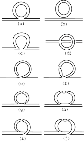
Figure 3: The quark level diagrams that could contribute to the 1-loop meson self energy. Diagrams (b) and (c), which require vertices of the form of Fig. 4(c), do not occur in the case of interest. Similarly, (d) only contributes to flavor-neutral propagators. Note that (f), (h) and (j) correspond to (e), (g), and (i), respectively, with iteration of either $m_{0}^{2}$, $\delta^{\prime}_{V}$, or $\delta^{\prime}_{A}$ vertices. These diagrams are to be taken as including any number of iterations, thus multiple internal quark loops.

The terms “connected” and “disconnected” refer to the internal loop at the quark level. In other words, a disconnected diagram will have either an internal disconnected propagator (Figs. 3(g)-(j)) or a disconnected vertex (Fig. 3(e)), or both (Fig. 3(f)). The disconnected propagators correspond to one or more insertions of a two-point $\delta^{\prime}$ or $m^{2}_{0}$ vertex (i.e., $\mathcal{D}$ in eqs. (39), (40) and (42)); while the disconnected vertices are generated by the $\mathcal{U}\,^{\prime}$ term in the potential, as we will see below.

We will explicitly perform the partially quenched calculation. Here the quenched valence quarks (call them $x$ and $y$) will in general have different masses from the sea quarks $u$, $d$ and $s$. We will still refer to this as a “$4\!+\!4\!+\!4$” partially quenched theory, based on its dynamical quark content. The chiral Lagrangian needed has 5 flavors, but 2 flavors are dropped, by fiat, from loops. From this 5-flavor, partially quenched theory, we can find equivalent 3-flavor (what we call “full” theory) results by setting the valence quark masses equal to various sea quark masses.

The valence quarks $x$ and $y$ form new mesons in our theory, which we name as follows:

$$X = x\bar{x}\qquad Y=y\bar{y}$$

$$P^{+} = x\bar{y}\qquad P^{-}=y\bar{x}\ .$$ (45)

We will not give individual names to the mesons formed from various valence-sea combinations such as $x\bar{u}$, but just refer to them generically by “$Q$.” A check on our final calculation here is that the 1-loop correction to $m_{P^{+}_{5}}^{2}$ should be proportional to $m_{x}+m_{y}$ (and hence $m_{P^{+}_{5}}^{2}$ itself), due to the separate $U_{A}(1)$ symmetries for $x$ and $y$ and the $x\leftrightarrow y$ interchange symmetry.

Since the mass, kinetic, and $\mathcal{U}$ terms are composed entirely of single traces, the relevant 4-meson vertices that they generate are all of the form of Figs. 4(a) and (b). (This is because “touching” flavor indices must be the same in a single trace.) In Fig. 4(b) the vertical meson lines must join to make the internal loop; however, they can only join with a disconnected propagator because they have different flavors. Thus connected contributions from mass, kinetic, and $\mathcal{U}$ all involve the vertex of Fig. 4(a), and produce diagrams of the form of Fig. 3(a). Disconnected contributions can come from Figs. 4(a) and (b).

The $\mathcal{U}\,^{\prime}$ terms, on the other hand, involve two traces, and therefore generate disconnected vertices, which in principle can be of the form of either Fig. 4(c) or (d). However it is not hard to show, from the explicit taste structure of $\mathcal{U}\,^{\prime}$, that only vertices with odd number of mesons coming from each trace contribute when two of the mesons are Goldstone particles (pseudoscalar taste). The $\mathcal{U}\,^{\prime}$ vertices then separate into two disconnected pieces, one with a single meson and the other with three. Thus $\mathcal{U}\,^{\prime}$ vertices must be of the form of Fig. 4(d), and not (c). This in turn implies that the $\mathcal{U}\,^{\prime}$ self energy diagrams have the disconnected structure of Fig. 3(e) or (f) only, where (e) uses a connected propagator and (f), a disconnected one.

Combining the connected contributions, we find:

$$\sigma^{con}(p^{2}) = -\frac{1}{12}\sum_{Q,B}\int\frac{d^{4}q}{\pi^{2}}\biggl{[}p^{2}+q^{2}+\left(m^{2}_{P^{+}_{5}}+m^{2}_{Q_{5}}\right)+a^{2}\Delta(\xi_{B})\biggr{]}\frac{1}{q^{2}+m^{2}_{Q_{B}}}.$$ (46)

As before, $B$ takes on the taste values {5, $\mu 5$, $\mu\nu\ (\mu<\nu),\ \mu,\ I$}, and $Q$ runs over all meson flavors with one valence quark ($x$ or $y$) and one sea quark ($u$, $d$, or $s$). Which mesons contribute is clear from Fig. 3(a). The first two terms in eq. (46) come from the kinetic energy: one from the derivatives acting on the external legs and the other from the derivatives acting on the internal loop. The last two terms are from the mass term and $\mathcal{U}$ respectively. We have used the fact that $\mu(m_{x}+m_{y})=m_{P^{+}_{5}}^{2}$ to rewrite the mass-term contribution.

The one-loop mass renormalization is just the self energy with the external momentum $p^{2}$ evaluated at $-m_{P^{+}_{5}}^{2}$. Making this substitution and noting from eq. (30) that $m^{2}_{Q_{B}}=m^{2}_{Q_{5}}+a^{2}\Delta(\xi_{B})$, the term inside the square brackets becomes $q^{2}+m^{2}_{Q_{B}}$, which cancels the denominator from the propagator. Thus, no chiral logarithms arise from these terms. This corresponds to the fact that all diagrams of the form of Fig. 3(a) cancel in the standard continuum chiral logarithm calculation GASSER_LEUTWYLER . (See Ref. CHIRAL_FSB for more discussion.)

For the disconnected contributions, it will be convenient to divide up $\sigma^{disc}$ further, according to (1) whether the particle in the loop is a vector, axial-vector, or singlet in taste, and (2) the type of diagram that generates the term. We thus have

$$\sigma^{disc}=\sigma^{disc}_{V}+\sigma^{disc}_{A}+\sigma^{disc}_{I}\ ,$$ (47)

with

$$\sigma_{V}^{disc} = \sigma_{V,gh}+\sigma_{V,ij}+\sigma_{V,e}+\sigma_{V,f}$$

$$\sigma_{A}^{disc} = \sigma_{A,gh}+\sigma_{A,ij}+\sigma_{A,e}+\sigma_{A,f}$$

$$\sigma_{I}^{disc} = \sigma_{I,gh}+\sigma_{I,ij}\ .$$ (48)

Here, the labels $gh$, $ij$, $e$, and $f$ refer to the diagrams in Fig. 3 that generate the contribution. As discussed above, the $gh$ and $ij$ contributions come from kinetic energy, mass, or $\mathcal{U}$ vertices, with a disconnected propagator. The $e$ and $f$ contributions have a $\mathcal{U}\,^{\prime}$ vertex and a connected or disconnected propagator, respectively. As is easily seen from the form eq. (18), $\mathcal{U}\,^{\prime}$ vertices that have two Goldstone mesons on the external lines must have only taste-vector or axial mesons on the loop. Therefore, $\sigma_{I}^{disc}$ gets contributions from Fig. 3(g)–(j) only, as it does in the continuum.

We focus first on the taste-vector contributions. $\sigma_{V,e}$ uses the vertex Fig. 4(d) with $i=x$ (or $i$=$y$ in its $x\to y$ variant) in order to have a connected propagator. We find, therefore,

$$\sigma_{V,e} = -\frac{2}{3}a^{2}\delta^{\prime}_{V}\int\frac{d^{4}q}{\pi^{2}}\biggl{[}\frac{1}{q^{2}+m^{2}_{X_{V}}}+\frac{1}{q^{2}+m^{2}_{Y_{V}}}\biggr{]}\ ,$$ (49)

where all but the overall coefficient follows immediately from the form of the diagram. We have already included the factor of 4 for the four degenerate taste-vector mesons, and will continue to do so below.

$\sigma_{V,f}$ again uses the vertex Fig. 4(d), but now $i$ must be one of the sea quarks, since a virtual quark loop is involved. The propagator is the disconnected taste-vector propagator, $\mathcal{D}^{V}$, eq. (39). We have

$$\sigma_{V,f}=-\frac{2}{3}a^{2}\delta^{\prime}_{V}\int\frac{d^{4}q}{\pi^{2}}\sum_{M=U,D,S}\left(\mathcal{D}^{V}_{XM}+\mathcal{D}^{V}_{YM}\right)\ .$$ (50)

Note that both $\sigma_{V,e}$ and $\sigma_{V,f}$ have explicit factors of $\delta^{\prime}_{V}$. These come from the 4-meson vertex, generated by $\mathcal{U}^{\prime}$. There are additional implicit factors of $\delta^{\prime}_{V}$ in the disconnected propagator $\mathcal{D}^{V}$ in $\sigma_{V,f}$. It is not immediately obvious that this same linear combination of $C_{2V}$ and $C_{5V}$ (see eq. (32)) must occur in both the 2-meson and 4-mesons vertices. However, we will see below that it is necessary for the cancellations that allow the ${P^{+}_{5}}$ mass renormalization to be proportional to $m^{2}_{P^{+}_{5}}$, as required by axial symmetry.

$\sigma_{V,gh}$ is generated by vertices of type Fig. 4(a), with $i=y$ (or $i$=$x$ in its $y\to x$ variant). The result is

$$\sigma_{V,gh}(p^{2}) = -\frac{1}{3}\int\frac{d^{4}q}{\pi^{2}}\Biggl{[}\left(p^{2}+q^{2}+m^{2}_{P^{+}_{5}}+m^{2}_{X_{5}}+a^{2}\Delta_{V}\right)\mathcal{D}^{V}_{XX}$$ (51)

$$\qquad+\left(p^{2}+q^{2}+m^{2}_{P^{+}_{5}}+m^{2}_{Y_{5}}+a^{2}\Delta_{V}\right)\mathcal{D}^{V}_{YY}\Biggr{]}\ .$$

The $p^{2}+q^{2}$ terms come from the kinetic energy vertex; $m^{2}_{P^{+}_{5}}$, $m^{2}_{X_{5}}$ and $m^{2}_{Y_{5}}$, from the mass vertex; and the $\Delta_{V}$ terms, from $\mathcal{U}$. Putting $p^{2}=-m^{2}_{P^{+}_{5}}$, and using $m^{2}_{X_{V}}=m^{2}_{X_{5}}+a^{2}\Delta_{V}$, from eq. (30), this simplifies to:

$$\sigma_{V,gh}(-m^{2}_{P^{+}_{5}})=-\frac{1}{3}\int\frac{d^{4}q}{\pi^{2}}\Biggl{[}\left(q^{2}+m^{2}_{X_{V}}\right)\mathcal{D}^{V}_{XX}\ +\left(q^{2}+m^{2}_{Y_{V}}\right)\mathcal{D}^{V}_{YY}\Biggr{]}\ .$$ (52)

Finally, we have $\sigma_{V,ij}$. This contribution uses the vertex Fig. 4(b) and, clearly, an $X$-$Y$ disconnected propagator.

$$\sigma_{V,ij}(p^{2}) = -\frac{2}{3}\int\frac{d^{4}q}{\pi^{2}}\Biggl{[}\left(p^{2}+q^{2}-m^{2}_{P^{+}_{5}}+a^{2}\Delta_{V}\right)\mathcal{D}^{V}_{XY}\Biggr{]}$$

$$\sigma_{V,ij}(-m^{2}_{P^{+}_{5}}) = -\frac{2}{3}\int\frac{d^{4}q}{\pi^{2}}\Biggl{[}\left(q^{2}-2m^{2}_{P^{+}_{5}}+a^{2}\Delta_{V}\right)\mathcal{D}^{V}_{XY}\Biggr{]}\ .$$ (53)

The sum of all the contributions to $\sigma^{disc}_{V}$ can be simplified with an identity derived by combining eqs. (38) and (41):

$$\sum_{M=U,D,S}\mathcal{D}^{V}_{XM}=-\frac{1}{q^{2}+m^{2}_{X_{V}}}-\frac{q^{2}+m^{2}_{X_{V}}}{a^{2}\delta^{\prime}_{V}}\mathcal{D}^{V}_{XX}\ .$$ (54)

Using this and the $X\leftrightarrow Y$ version we can add eq. (50) to eqs. (49) and (52). The trivial identity (from eq. (39))

$$(q^{2}+m^{2}_{X_{V}})\mathcal{D}^{V}_{XX}=(q^{2}+m^{2}_{Y_{V}})\mathcal{D}^{V}_{XY}$$ (55)

and the fact that $m^{2}_{X_{V}}+m^{2}_{Y_{V}}=2m^{2}_{P^{+}_{V}}=2m^{2}_{P^{+}_{5}}+2a^{2}\Delta_{V}$, can then be used to combine the result with eq. (III) to give simply

$$\sigma^{disc}_{V}(-m^{2}_{P^{+}_{5}})=2m^{2}_{P^{+}_{5}}\int\frac{d^{4}q}{\pi^{2}}\mathcal{D}^{V}_{XY}\ .$$ (56)

Note that the result is proportional to $m^{2}_{P^{+}_{5}}$, as expected. The corresponding expression for $\sigma^{disc}_{A}$ is obtained by $V\to A$.

For $\sigma^{disc}_{I}$, we just have contributions from Figs. 3(g)–(j). These contributions are very similar to the corresponding ones for $\sigma^{disc}_{V}$. We have:

$$\sigma_{I,gh}(p^{2}) = -\frac{1}{12}\int\frac{d^{4}q}{\pi^{2}}\Biggl{[}\left(p^{2}+q^{2}+m^{2}_{P^{+}_{5}}+m^{2}_{X_{5}}+a^{2}\Delta_{I}\right)\mathcal{D}^{I}_{XX}$$

$$\ \qquad\qquad+\left(p^{2}+q^{2}+m^{2}_{P^{+}_{5}}+m^{2}_{Y_{5}}+a^{2}\Delta_{I}\right)\mathcal{D}^{I}_{YY}\Biggr{]}$$

$$\sigma_{I,gh}(-m^{2}_{P^{+}_{5}}) = -\frac{1}{12}\int\frac{d^{4}q}{\pi^{2}}\left[\left(q^{2}+m^{2}_{X_{I}}\right)\mathcal{D}^{I}_{XX}+\left(q^{2}+m^{2}_{Y_{I}}\right)\mathcal{D}^{I}_{YY}\right]$$ (57)

$$\sigma_{I,ij}(p^{2}) = \frac{1}{6}\int\frac{d^{4}q}{\pi^{2}}\left[\left(p^{2}+q^{2}-m^{2}_{P^{+}_{5}}+a^{2}\Delta_{I}\right)\right]\mathcal{D}^{I}_{XY}$$

$$\sigma_{I,ij}(-m^{2}_{P^{+}_{5}}) = \frac{1}{6}\int\frac{d^{4}q}{\pi^{2}}\left[\left(q^{2}-2m^{2}_{P^{+}_{5}}+a^{2}\Delta_{I}\right)\right]\mathcal{D}^{I}_{XY}\ ,$$ (58)

The $V\to I$ version of eq. (55) allows us to combine eqs. (57) and (58), yielding

$$\sigma^{disc}_{I}(-m^{2}_{P^{+}_{5}})=-\frac{m^{2}_{P^{+}_{5}}}{2}\int\frac{d^{4}q}{\pi^{2}}\mathcal{D}^{I}_{XY}$$ (59)

Again, the result is proportional to $m^{2}_{P^{+}_{5}}$.

Collecting eqs. (56) and (59) according to eq. (47), gives

$$\sigma^{disc}(-m^{2}_{P^{+}_{5}})=\frac{m^{2}_{P^{+}_{5}}}{2}\int\frac{d^{4}q}{\pi^{2}}\left(4\mathcal{D}^{V}_{XY}+4\mathcal{D}^{A}_{XY}-\mathcal{D}^{I}_{XY}\right)\ .$$ (60)

Since $\sigma^{con}$ is just a quarticly divergent constant, the above result contains all the 1-loop chiral logarithms in the mass renormalization.

The result in eq. (60) is rather implicit. To express the chiral logarithms more concretely, we would need three further steps:

• (1) find the explicit expressions for the eigenvalues of the full mass matrices in the denominators of the $\mathcal{D}$ (e.g., $m^{2}_{\pi^{0}_{V}}$, $m^{2}_{\eta_{V}}$ and $m^{2}_{\eta^{\prime}_{V}}$ in $\mathcal{D}^{V}$).

• (2) take the $m_{0}^{2}\to\infty$ limit in the taste-singlet term.

• (3) write the disconnected propagators $\mathcal{D}$ as sums of simple poles and perform the integrals over $q$.

Steps (1) and (2) are slightly different in the $1\!+\!1\!+\!1$ case of interest than in the present $4\!+\!4\!+\!4$ case, so we postpone them until later. On the other hand, step (3) can be done quite generally, so we present it here.

The integrands in eq. (60) are of the form

$$\mathcal{I}^{[n,k]}\left(\left\{m\right\}\!;\!\left\{\mu\right\}\right)\equiv\frac{\prod_{a=1}^{k}(q^{2}+\mu^{2}_{a})}{\prod_{j=1}^{n}(q^{2}+m^{2}_{j})}\ ,$$ (61)

where $\{m\}$ and $\{\mu\}$ are the sets of masses $\{m_{1},m_{2},\dots,m_{n}\}$ and $\{\mu_{1},\mu_{2},\dots,\mu_{k}\}$. respectively. As long as there are no mass degeneracies in the denominator, and $n>k$ (which is true here even after the $m_{0}^{2}\to\infty$ limit), $\mathcal{I}{[n,k]}$ can be written as the sum of simple poles times their residues:

$$\mathcal{I}^{[n,k]}\left(\left\{m\right\}\!;\!\left\{\mu\right\}\right)=\sum_{j=1}^{n}\frac{R_{j}^{[n,k]}\left(\left\{m\right\}\!;\!\left\{\mu\right\}\right)}{q^{2}+m^{2}_{j}}\ ,$$ (62)

where

$$R_{j}^{[n,k]}\left(\left\{m\right\}\!;\!\left\{\mu\right\}\right)\equiv\frac{\prod_{a=1}^{k}(\mu^{2}_{a}-m^{2}_{j})}{\prod_{i\not=j}(m^{2}_{i}-m^{2}_{j})}\ .$$ (63)

Equation (62) just follows from the fact that an analytic function is determined by its poles and behavior at infinity; it is known as “Lagrange’s formula” in complex analysis LAGRANGE .

The integrals of the simple poles can now be done using

$$\mathcal{I}_{1}\equiv\int\frac{d^{4}q}{(2\pi)^{4}}\frac{1}{q^{2}+m^{2}}\rightarrow\frac{1}{16\pi^{2}}\ell(m^{2})\ ,$$ (64)

where

$$\ell(m^{2})\equiv m^{2}\ln\frac{m^{2}}{\Lambda^{2}}\qquad{\rm[infinite\ volume]}\ ,$$ (65)

with $\Lambda$ the chiral scale. We use the arrow in eq. (64) and later to indicate that we are only keeping the chiral logarithm terms. If the system is in a finite (but large) spatial volume $L^{3}$, we only have to modify eq. (65):

$$\ell(m^{2})\equiv m^{2}\left(\ln\frac{m^{2}}{\Lambda^{2}}+\delta_{1}(mL)\right)\qquad{\rm[finite\ spatial\ volume]}\ ,$$ (66)

where CHIRAL_FSB

$$\delta_{1}(mL)=\frac{4}{mL}\sum_{\vec{r}\neq 0}\frac{K_{1}(|\vec{r}|mL)}{|\vec{r}|}\ ,$$ (67)

with $K_{1}$ the Bessel function of imaginary argument.

With the above, we can write a general integral of the form in eq. (60) as

$$\int\frac{d^{4}q}{\pi^{2}}\mathcal{I}^{[n,k]}\left(\left\{m\right\}\!;\!\left\{\mu\right\}\right)\rightarrow\sum_{j=1}^{n}{R_{j}^{[n,k]}\left(\left\{m\right\}\!;\!\left\{\mu\right\}\right)}\ \ell(m_{j}^{2})\ .$$ (68)

We make one final comment on the $4\!+\!4\!+\!4$ calculation before going on to the $1\!+\!1\!+\!1$ case. In Ref. CHIRAL_FSB , certain chiral logarithm terms were claimed to come from pure valence diagrams, with connected propagators; while in the current calculation, all such terms cancel. What is the reason for the discrepancy? As discussed above, the problem in CHIRAL_FSB was the incorrect treatment of flavor indices. Because of this, it was not realized that there is a difference between a propagator of a flavor-neutral Goldstone pion, such as $U_{5}$, and that of the flavor-nonsinglet $\pi^{+}_{5}$ (or between their partially quenched counterparts, $X_{5}$ and $P^{+}_{5}$). An explicit computation in the current framework shows that the connected, valence terms found in CHIRAL_FSB do in fact exist, but only for a flavor-neutral propagator. Such terms arise identically in the $X_{5}$-$Y_{5}$, $X_{5}$-$X_{5}$, and $Y_{5}$-$Y_{5}$ propagators, but do not appear in the $P^{+}_{5}$-$P^{-}_{5}$ propagator. This proves that they come from Fig. 3(d). The needed vertex is Fig. 4(b) (after relabeling), which is generated by kinetic, mass and $\mathcal{U}$ terms. The claim in CHIRAL_FSB that connected, valence terms come from Fig. 3(c) with vertex Fig. 4(c) is incorrect. Indeed, it was argued above that the flavor structure of the terms in our Lagrangian forbids vertex Fig. 4(c), at least with two external Goldstone mesons.

IV Moving from $4\!+\!4\!+\!4$ to $1\!+\!1\!+\!1$ dynamical flavors

To make the $4\!+\!4\!+\!4$ result, eq. (60), into a $1\!+\!1\!+\!1$ result, we simply must divide by a factor of 4 for every sea quark loop. The contributing diagrams are Figs. 3 (e)–(j). There can be either taste-vector, taste-axial vector or taste-singlet mesons on the internal lines of these diagrams, and we can treat all these cases at the same time simply by defining

$$\delta^{\prime}=\cases{a^{2}\delta^{\prime}_{V},&taste-vector;\cr a^{2}\delta^{\prime}_{A},&taste-axial;\cr 4m_{0}^{2}/3,&taste-singlet.\cr}$$ (69)

Diagrams (e), (g), and (i) have no sea quark loops and a single factor of $\delta^{\prime}$ (in (e) this comes from the 4-meson $\mathcal{U}\,^{\prime}$ vertex). Diagrams (f), (h), and (j) have one additional factor of $\delta^{\prime}$ for each sea quark loop. Therefore, dividing by 4 for every sea quark loop is the same as dividing every factor of $\delta^{\prime}$, except the first, by 4. For a general function $f(\delta^{\prime})$ which vanishes linearly as $\delta^{\prime}\rightarrow 0$, we can make this adjustment simply by the replacement $f(\delta^{\prime})\rightarrow 4f\left(\frac{\delta^{\prime}}{4}\right)$. Alternatively, we can see from eqs. (60), (39) and (42) that the first factor of $\delta^{\prime}$ comes from the explicit $\delta^{\prime}$ in front of $\mathcal{D}^{V}$, $\mathcal{D}^{A}$ or $\mathcal{D}^{I}$; while higher order terms in $\delta^{\prime}$ are implicit in the values of the “full” masses in the denominators relative to the “unmixed” masses in the numerators. Therefore, to go from $4\!+\!4\!+\!4$ to $1\!+\!1\!+\!1$, we leave the explicit $\delta^{\prime}$ factors alone but merely let $\delta^{\prime}\to\delta^{\prime}/4$ before diagonalizing the full mass matrix.

The full mass matrices to be diagonalized follow from the flavor-neutral mixing term in $\mathcal{L}$, written down following eqs. (32) and (33). After $\delta^{\prime}\to\delta^{\prime}/4$, these have the form

$$\left(\matrix{m^{2}_{U}+\delta^{\prime}/4&\delta^{\prime}/4&\delta^{\prime}/4\cr\delta^{\prime}/4&m^{2}_{D}+\delta^{\prime}/4&\delta^{\prime}/4\cr\delta^{\prime}/4&\delta^{\prime}/4&m^{2}_{S}+\delta^{\prime}/4\cr}\right)$$ (70)

Here the masses $m^{2}_{U}$, $m^{2}_{D}$, $m^{2}_{S}$ have an implicit taste label ($V$, $A$, or $I$) depending on which case we are considering. The explicit expressions for the eigenvalues of eq. (70) are complicated and not illuminating in general. The solutions in the $2\!+\!1$ ($m_{u}=m_{d}$) case, however, have simple forms, and that is the case of greatest current interest. In the taste-vector channel, we have, for the $2\!+\!1$ case,

$$m_{\pi^{0}_{V}}^{2} = m_{U_{V}}^{2}=m_{D_{V}}^{2}\ ,$$

$$m_{\eta_{V}}^{2} = \frac{1}{2}\left(m_{U_{V}}^{2}+m_{S_{V}}^{2}+\frac{3}{4}a^{2}\delta^{\prime}_{V}-Z\right)\ ,$$

$$m_{\eta^{\prime}_{V}}^{2} = \frac{1}{2}\left(m_{U_{V}}^{2}+m_{S_{V}}^{2}+\frac{3}{4}a^{2}\delta^{\prime}_{V}+Z\right)\ ;$$ (71)

$$Z \equiv \sqrt{\left(m_{S_{V}}^{2}-m_{U_{V}}^{2}\right)^{2}-\frac{a^{2}\delta^{\prime}_{V}}{2}\left(m_{S_{V}}^{2}-m_{U_{V}}^{2}\right)+\frac{9(a^{2}\delta^{\prime}_{V})^{2}}{16}}$$

The taste-axial case just requires $V\to A$. In the taste-singlet case, $\delta^{\prime}=4m_{0}^{2}/3$, and $m_{0}^{2}$ will be taken to infinity, so only the large-$m_{0}$ expressions are needed. We have (again for $2\!+\!1$):

$$m_{\pi^{0}_{I}}^{2} = m_{U_{I}}^{2}=m^{2}_{D_{I}}$$

$$m_{\eta_{I}}^{2} = \frac{m_{U_{I}}^{2}}{3}+\frac{2m_{S_{I}}^{2}}{3}$$ (72)

$$m_{\eta^{\prime}_{I}}^{2} = m_{0}^{2}\ ,$$

where we have neglected corrections that are $\mathcal{O}(1/m_{0}^{2})$ compared to the terms kept.

Finally, we can give the result for the chiral logs in the Goldstone pion self energy. For the moment we stay with the partially quenched expression and also assume no degeneracies among the valence and sea quark masses. In the $1\!+\!1\!+\!1$ case we obtain from eq. (60) with eqs. (39), (42) and (44):

$$\Sigma^{1+1+1}(-m^{2}_{P_{5}^{+}}) \rightarrow \frac{m^{2}_{P_{5}^{+}}}{16\pi^{2}f^{2}}\Big{(}-2a^{2}\delta^{\prime}_{V}\sum_{j_{V}}R^{[5,3]}_{j_{V}}\;\ell(m^{2}_{j_{V}})-2a^{2}\delta^{\prime}_{A}\sum_{j_{A}}R^{[5,3]}_{j_{A}}\;\ell(m^{2}_{j_{A}})$$ (73)

$$\qquad\qquad+\frac{2}{3}\sum_{j_{I}}R^{[4,3]}_{j_{I}}\;\ell(m^{2}_{j_{I}})\Big{)}\ ,$$

where we have used eq. (68), and $R_{j}^{n,k}$ and $\ell(m^{2})$ are given by eqs. (63) and (65) or (66). $j_{V}$ runs over $\{{X_{V}},{Y_{V}},{\pi^{0}_{V}},{\eta_{V}},{\eta^{\prime}_{V}}\}$ and

$$R^{[5,3]}_{j_{V}}=R^{[5,3]}_{j_{V}}\left(\{m_{X_{V}},m_{Y_{V}},m_{\pi^{0}_{V}},m_{\eta_{V}},m_{\eta^{\prime}_{V}}\};\{m_{U_{V}},m_{D_{V}},m_{S_{V}}\}\right)\ .$$ (74)

(For $R^{[5,3]}_{j_{A}}$, just let $V\to A$). Similarly, $j_{I}$ runs over $\{{X_{I}},{Y_{I}},{\pi^{0}_{I}},{\eta_{I}}\}$ (the $\eta^{\prime}_{I}$ has decoupled in the $m_{0}^{2}\to\infty$ limit), and

$$R^{[4,3]}_{j_{I}}=R^{[4,3]}_{j_{I}}\left(\{m_{X_{I}},m_{Y_{I}},m_{\pi^{0}_{I}},m_{\eta_{I}}\};\{m_{U_{I}},m_{D_{I}},m_{S_{I}}\}\right)\ .$$ (75)

In each taste channel, the values of $m^{2}_{\pi^{0}}$, $m^{2}_{\eta}$, and $m^{2}_{\eta^{\prime}}$ in eq. (73) are just the eigenvalues of the corresponding version of eq. (70).

The $2\!+\!1$ ($m_{u}=m_{d}$) case is very similar, but because $m_{\pi^{0}}^{2}=m_{U}^{2}=m_{D}^{2}$, there is a cancellation in eqs. (39) and (42) between $q^{2}+m_{\pi^{0}}^{2}$ in the denominators and, say, $q^{2}+m_{D}^{2}$ in the numerators. Assuming no other degeneracies, we have

$$\Sigma^{2+1}(-m^{2}_{P_{5}^{+}}) \rightarrow \frac{m^{2}_{P_{5}^{+}}}{16\pi^{2}f^{2}}\Big{(}-2a^{2}\delta^{\prime}_{V}\sum_{j_{V}}R^{[4,2]}_{j_{V}}\;\ell(m^{2}_{j_{V}})-2a^{2}\delta^{\prime}_{A}\sum_{j_{A}}R^{[4,2]}_{j_{A}}\;\ell(m^{2}_{j_{A}})$$ (76)

$$\qquad\qquad+\frac{2}{3}\sum_{j_{I}}R^{[3,2]}_{j_{I}}\;\ell(m^{2}_{j_{I}})\Big{)}\ .$$

Here $j_{V}$ runs over $\{{X_{V}},{Y_{V}},{\eta_{V}},{\eta^{\prime}_{V}}\}$ and

$$R^{[4,2]}_{j_{V}}=R^{[4,2]}_{j_{V}}\left(\{m_{X_{V}},m_{Y_{V}},m_{\eta_{V}},m_{\eta^{\prime}_{V}}\};\{m_{U_{V}},m_{S_{V}}\}\right)\ .$$ (77)

Again, let $V\to A$ for $R^{[4,2]}_{j_{A}}$. The index $j_{I}$ runs over $\{{X_{I}},{Y_{I}},{\eta_{I}}\}$, and

$$R^{[3,2]}_{j_{I}}=R^{[3,2]}_{j_{I}}\left(\{m_{X_{I}},m_{Y_{I}},m_{\eta_{I}}\};\{m_{U_{I}},m_{S_{I}}\}\right)\ .$$ (78)

In this case, the values of $m^{2}_{\pi^{0}}$, $m^{2}_{\eta}$, and $m^{2}_{\eta^{\prime}}$ are given by eqs. (IV) and (IV).

Cases of interest with further degeneracies (such as a “full” $2\!+\!1$ pion with $m_{x}=m_{y}=m_{u}=m_{d}$) can be obtained by carefully taking limits in eq. (76). We will write down some of these cases explicitly in Sec. VI, where we also include the analytic contributions.

V Quenched Case

Since we can think of the quenched theory as the limit of the partially quenched theory as the sea quark masses go to infinity, all the manipulations that led to eq. (60) will go through unscathed in the quenched case. We can therefore simply replace the disconnected propagators in eq. (60) with their quenched versions, eqs. (40) and (43). Using the same notation as in eqs. (73) and (76), we have (assuming $m_{x}\not=m_{y}$):

$$\Sigma^{\rm quench}(-m^{2}_{P_{5}^{+}}) \rightarrow \frac{m^{2}_{P_{5}^{+}}}{16\pi^{2}f^{2}}\Big{(}-2a^{2}\delta^{\prime}_{V}\sum_{j_{V}}R^{[2,0]}_{j_{V}}\;\ell(m^{2}_{j_{V}})-2a^{2}\delta^{\prime}_{A}\sum_{j_{A}}R^{[2,0]}_{j_{A}}\;\ell(m^{2}_{j_{A}})$$ (79)

$$\qquad\qquad+\frac{2}{3}\sum_{j_{I}}R^{[2,0]}_{j_{I}}\;(m_{0}^{2}-\alpha m^{2}_{j_{I}})\ell(m^{2}_{j_{I}})\Big{)}\ .$$

Here $j_{V}$ runs over $\{{X_{V}},{Y_{V}}\}$; similarly for $j_{A}$ and $j_{I}$. For the $\alpha$-dependent terms, we have used the integral

$$\mathcal{I}_{2}\equiv\int\frac{d^{4}q}{(2\pi)^{4}}\frac{q^{2}}{q^{2}+m^{2}}=-m^{2}\mathcal{I}_{1}+\int\frac{d^{4}q}{(2\pi)^{4}}\rightarrow-\frac{1}{16\pi^{2}}m^{2}\ell(m^{2})\ ,$$ (80)

where $\mathcal{I}_{1}$ is defined in eq. (64).

Because the quenched residues here are particularly simple, it is useful to write out the result more explicitly:

$$\Sigma^{\rm quench}(-m^{2}_{P_{5}^{+}}) \rightarrow \frac{m^{2}_{P_{5}^{+}}}{16\pi^{2}f^{2}}\Biggl{[}-2a^{2}\delta^{\prime}_{V}\frac{\ell(m^{2}_{X_{V}})-\ell(m^{2}_{Y_{V}})}{m^{2}_{Y_{V}}-m^{2}_{X_{V}}}-2a^{2}\delta^{\prime}_{A}\frac{\ell(m^{2}_{X_{A}})-\ell(m^{2}_{Y_{A}})}{m^{2}_{Y_{A}}-m^{2}_{X_{A}}}$$ (81)

$$+\frac{2}{3}\frac{(m_{0}^{2}-\alpha m^{2}_{X_{I}})\ell(m^{2}_{X_{I}})-(m_{0}^{2}-\alpha m^{2}_{Y_{I}})\ell(m^{2}_{Y_{I}})}{m^{2}_{Y_{I}}-m^{2}_{X_{I}}}\Biggr{]}.$$

VI Final one-loop results

The mass at one loop is given by

$$(m_{P^{+}_{5}}^{1-{\rm loop}})^{2}=m_{P^{+}_{5}}^{2}+\Sigma(-m_{P^{+}_{5}}^{2})\ .$$ (82)

The chiral logarithm contributions to $\Sigma(-m_{P^{+}_{5}}^{2})$ are presented in eqs. (73), (76) and (81), but for complete one-loop expressions we also need the “$\mathcal{O}(p^{4})$” analytic terms. The latter are unchanged from Ref. CHIRAL_FSB . However, for the analytic coefficients we now prefer to use the more standard GASSER_LEUTWYLER $L_{i}$, rather than the parameters $K_{3}$ and $K^{\prime}_{4}$ employed in CHIRAL_FSB .

In the absence of any degeneracies, we have, in the $1\!+\!1\!+\!1$ case,

$$\frac{(m^{1-{\rm loop},\,1+1+1}_{P^{+}_{5}})^{2}}{\left(m_{x}+m_{y}\right)} = \mu\Biggl{\{}1+\frac{1}{16\pi^{2}f^{2}}\Big{(}-2a^{2}\delta^{\prime}_{V}\sum_{j_{V}}R^{[5,3]}_{j_{V}}\;\ell(m^{2}_{j_{V}})-2a^{2}\delta^{\prime}_{A}\sum_{j_{A}}R^{[5,3]}_{j_{A}}\;\ell(m^{2}_{j_{A}})$$ (83)

$$\qquad\qquad+\frac{2}{3}\sum_{j_{I}}R^{[4,3]}_{j_{I}}\;\ell(m^{2}_{j_{I}})\Big{)}+\frac{16\mu}{f^{2}}\left(2L_{8}-L_{5}\right)\left(m_{x}+m_{y}\right)$$

$$\qquad\qquad+\frac{32\mu}{f^{2}}\left(2L_{6}-L_{4}\right)\left(m_{u}+m_{d}+m_{s}\right)+a^{2}C\Biggr{\}}.$$

Definitions here are the same as in eq. (73); the chiral logarithm function $\ell(m^{2})$ is given by eq. (65), or in finite volume, by eq. (66). Recall that ours is a joint expansion in the quark masses (generically $m$) and $a^{2}$. The analytic terms in $(m^{1-{\rm loop}})^{2}$ here are $\mathcal{O}(m^{2})$ or $\mathcal{O}(ma^{2})$; $\mathcal{O}(a^{4})$ terms cannot enter here because the pion mass must vanish in the chiral limit. Lattice effects violating continuum rotational invariance cannot show up at this order for the Goldstone pion — see Appendix.

Similarly, for $m_{u}=m_{d}\equiv m_{l}$ (the $2\!+\!1$ case), but with no other degeneracies, we have

$$\frac{(m^{1-{\rm loop},\,2+1}_{P^{+}_{5}})^{2}}{\left(m_{x}+m_{y}\right)} = \mu\Biggl{\{}1+\frac{1}{16\pi^{2}f^{2}}\Big{(}-2a^{2}\delta^{\prime}_{V}\sum_{j_{V}}R^{[4,2]}_{j_{V}}\;\ell(m^{2}_{j_{V}})-2a^{2}\delta^{\prime}_{A}\sum_{j_{A}}R^{[4,2]}_{j_{A}}\;\ell(m^{2}_{j_{A}})$$ (84)

$$\qquad\qquad+\frac{2}{3}\sum_{j_{I}}R^{[3,2]}_{j_{I}}\;\ell(m^{2}_{j_{I}})\Big{)}+\frac{16\mu}{f^{2}}\left(2L_{8}-L_{5}\right)\left(m_{x}+m_{y}\right)$$

$$\qquad\qquad+\frac{32\mu}{f^{2}}\left(2L_{6}-L_{4}\right)\left(2m_{l}+m_{s}\right)+a^{2}C\Biggr{\}}.$$

Definitions here are the same as in eq. (76).

The quenched result is

$$\frac{(m^{1-{\rm loop},\,{\rm quench}}_{P^{+}_{5}})^{2}}{\left(m_{x}+m_{y}\right)} = \mu\Biggl{\{}1+\frac{1}{16\pi^{2}f^{2}}\Biggl{[}-2a^{2}\delta^{\prime}_{V}\frac{\ell(m^{2}_{X_{V}})-\ell(m^{2}_{Y_{V}})}{m^{2}_{Y_{V}}-m^{2}_{X_{V}}}-2a^{2}\delta^{\prime}_{A}\frac{\ell(m^{2}_{X_{A}})-\ell(m^{2}_{Y_{A}})}{m^{2}_{Y_{A}}-m^{2}_{X_{A}}}$$ (85)

$$\qquad\qquad+\frac{2}{3}\frac{(m_{0}^{2}-\alpha m^{2}_{X_{I}})\ell(m^{2}_{X_{I}})-(m_{0}^{2}-\alpha m^{2}_{Y_{I}})\ell(m^{2}_{Y_{I}})}{m^{2}_{Y_{I}}-m^{2}_{X_{I}}}\Biggr{]}$$

$$\qquad\qquad+\frac{16\mu}{f^{2}}\left(2L^{\prime}_{8}-L^{\prime}_{5}\right)\left(m_{x}+m_{y}\right)+a^{2}C^{\prime}\Biggr{\}},$$

where the primes on $L^{\prime}_{8}$, $L^{\prime}_{5}$, and $C^{\prime}$ indicate that they may have different values than in the unquenched cases. Of course, there is no analytic term involving the sea quarks ($2L^{\prime}_{6}-L^{\prime}_{4}$) in the quenched case.

It is useful to write down more explicit versions of the above results in various limits pertinent to many simulations. First, with $m_{u}\neq m_{d}$, we set $m_{x}=m_{u}$ and $m_{y}=m_{d}$ to obtain the “full QCD” charged pion mass in the $1\!+\!1\!+\!1$ case:

$$\frac{(m^{1-{\rm loop},\,1+1+1}_{\pi^{+}_{5}})^{2}}{\left(m_{u}+m_{d}\right)}\!\!\! =\mu\Biggl{\{}1+\frac{1}{16\pi^{2}f^{2}}\Biggl{[}-2a^{2}\delta^{\prime}_{V}\Biggl{(}\frac{m_{S_{V}}^{2}-m^{2}_{\pi^{0}_{V}}}{(m_{\eta_{V}}^{2}-m^{2}_{\pi^{0}_{V}})(m_{\eta^{\prime}_{V}}^{2}-m^{2}_{\pi^{0}_{V}})}\ell(m^{2}_{\pi^{0}_{V}})+$$ (86)

$$\frac{m_{S_{V}}^{2}-m^{2}_{\eta_{V}}}{(m_{\eta^{\prime}_{V}}^{2}-m^{2}_{\eta_{V}})(m_{\pi^{0}_{V}}^{2}-m^{2}_{\eta_{V}})}\ell(m^{2}_{\eta_{V}})+\frac{m_{S_{V}}^{2}-m^{2}_{\eta^{\prime}_{V}}}{(m_{\eta_{V}}^{2}-m^{2}_{\eta^{\prime}_{V}})(m_{\pi^{0}_{V}}^{2}-m^{2}_{\eta^{\prime}_{V}})}\ell(m^{2}_{\eta^{\prime}_{V}})\Biggr{)}$$

$$+\biggl{(}V\to A\biggr{)}+\frac{2}{3}\Biggl{(}\frac{m_{S_{I}}^{2}-m_{\pi^{0}_{I}}^{2}}{m_{\eta_{I}}^{2}-m_{\pi^{0}_{I}}^{2}}\ell(m_{\pi^{0}_{I}}^{2})+\frac{m_{S_{I}}^{2}-m_{\eta_{I}}^{2}}{m_{\pi^{0}_{I}}^{2}-m_{\eta_{I}}^{2}}\ell(m_{\eta_{I}}^{2})\Biggr{)}\Biggr{]}$$

$$\!\!\!\!\!\!\!\!\!\!+\frac{16\mu}{f^{2}}\left(2L_{8}-L_{5}\right)\left(m_{u}+m_{d}\right)+\frac{32\mu}{f^{2}}\left(2L_{6}-L_{4}\right)\left(m_{u}+m_{d}+m_{s}\right)+a^{2}C\Biggr{\}}.$$

This result is most easily obtained by taking the degenerate mass limits in eq. (60), before the integral is performed, rather than in eq. (83). The quantities $m^{2}_{\pi^{0}}$, $m^{2}_{\eta}$ and $m^{2}_{\eta^{\prime}}$ are eigenvalues of the mass matrix, eq. (70). From eq. (86) we can get the charged kaon mass simply by interchanging the explicit labels $d\leftrightarrow s$ and $D\leftrightarrow S$. (The neutral labels $\pi^{0}$, $\eta$, and $\eta^{\prime}$ are unaffected.)

The results for the full pion and kaon in the case of degenerate up and down quark masses (both set to $m_{l}$) are also of interest, as they are needed to fit many simulations. Since the pion and kaon results look quite different, we show them both:

$$\frac{(m^{1-{\rm loop},\,2+1}_{\pi^{+}_{5}})^{2}}{2m_{l}} = \mu\Biggl{\{}1+\frac{1}{16\pi^{2}f^{2}}\Biggl{(}\biggl{[}-4\ell(m^{2}_{\pi^{0}_{V}})-\frac{2a^{2}\delta^{\prime}_{V}}{m_{\eta^{\prime}_{V}}^{2}-m^{2}_{\eta_{V}}}\biggl{(}\frac{m_{S_{V}}^{2}-m^{2}_{\eta_{V}}}{m_{\pi^{0}_{V}}^{2}-m^{2}_{\eta_{V}}}\ell(m^{2}_{\eta_{V}})$$ (87)

$$-\frac{m_{S_{V}}^{2}-m^{2}_{\eta^{\prime}_{V}}}{m_{\pi^{0}_{V}}^{2}-m^{2}_{\eta^{\prime}_{V}}}\ell(m^{2}_{\eta^{\prime}_{V}})\biggr{)}\biggr{]}+\biggl{[}V\to A\biggr{]}+\ell(m_{\pi^{0}_{I}}^{2})-\frac{1}{3}\ell(m_{\eta_{I}}^{2})\Biggr{)}$$

$$+\frac{16\mu}{f^{2}}\left(2L_{8}-L_{5}\right)\left(2m_{l}\right)+\frac{32\mu}{f^{2}}\left(2L_{6}-L_{4}\right)\left(2m_{l}+m_{s}\right)+a^{2}C\Biggr{\}},$$

$$\frac{(m^{1-{\rm loop},\,2+1}_{K^{+}_{5}})^{2}}{(m_{l}+m_{s})} = \mu\Biggl{\{}1+\frac{1}{16\pi^{2}f^{2}}\Biggl{(}\biggl{[}-\frac{2a^{2}\delta^{\prime}_{V}}{m_{\eta^{\prime}_{V}}^{2}-m^{2}_{\eta_{V}}}\biggl{(}\ell(m^{2}_{\eta_{V}})-\ell(m^{2}_{\eta^{\prime}_{V}})\biggr{)}\biggr{]}+\biggl{[}V\to A\biggr{]}$$ (88)

$$\qquad\qquad\qquad+\frac{2}{3}\ell(m_{\eta_{I}}^{2})\Biggr{)}+\frac{16\mu}{f^{2}}\left(2L_{8}-L_{5}\right)\left(m_{l}+m_{s}\right)$$

$$\qquad\qquad\qquad\qquad+\frac{32\mu}{f^{2}}\left(2L_{6}-L_{4}\right)\left(2m_{l}+m_{s}\right)+a^{2}C\Biggr{\}}.$$

Again, the relevant limits are most easily taken before the integrals are performed. The $\pi^{0}$, $\eta$ and $\eta^{\prime}$ masses in this case are given explicitly in eqs. (IV) and (IV); we have made heavy use of these explicit forms to simplify the chiral logarithm terms in the $\pi$ mass.

The last case we will look at is the quenched pion mass correction in the limit of degenerate valence masses ($m_{y}=m_{x}$). Here we get a double pole in the pion self energy. We can either carefully take the limit $m_{y}\to m_{x}$ in eq. (85), or return to eq. (60) with quenched $\mathcal{D}$ terms and do the double pole integrals directly. We follow the latter approach. We need the following integrals:

$$\mathcal{I}_{3} \equiv \int\frac{d^{4}q}{(2\pi)^{4}}\frac{1}{(q^{2}+m^{2})^{2}}=-\frac{\partial}{\partial m^{2}}\mathcal{I}_{1}\rightarrow\frac{1}{16\pi^{2}}\tilde{\ell}(m^{2})\ ,$$ (89)

$$\mathcal{I}_{4} \equiv \int\frac{d^{4}q}{(2\pi)^{4}}\frac{q^{2}}{(q^{2}+m^{2})^{2}}=\mathcal{I}_{1}-m^{2}\mathcal{I}_{3}\rightarrow\frac{1}{16\pi^{2}}\left(\ell(m^{2})-m^{2}\tilde{\ell}(m^{2})\right)\ ,$$ (90)

where $\mathcal{I}_{1}$ is given in eq. (64); $\ell(m^{2})$, in eq. (65); and

$$\tilde{\ell}(m^{2})\equiv-\left(\ln\frac{m^{2}}{\Lambda^{2}}+1\right)\qquad{\rm[infinite\ volume]}\ ,$$ (91)

with $\Lambda$ the chiral scale. In finite spatial volume $L^{3}$,

$$\tilde{\ell}(m^{2})\equiv-\left(\ln\frac{m^{2}}{\Lambda^{2}}+1\right)+\delta_{3}(mL)\qquad{\rm[finite\ spatial\ volume]}\ ,$$ (92)

where CHIRAL_FSB

$$\delta_{3}(mL)=2\sum_{\vec{r}\neq 0}K_{0}(|\vec{r}|mL)\ ,$$ (93)

with $K_{0}$ the Bessel function of imaginary argument. Note that the $+1$ term in $\tilde{\ell}(m^{2})$ was omitted in Ref. CHIRAL_FSB . That is formally acceptable when we are only keeping chiral logarithms, but inconvenient, since then the result from performing the double pole integral is not equal to degenerate limit of the chiral logs from the single poles.

Using the above integrals, we get:

$$\frac{(m^{1-{\rm loop},\,{\rm quench}}_{P^{+}_{5}})^{2}}{2m_{x}} = \mu\Biggl{\{}1+\frac{1}{16\pi^{2}f^{2}}\Biggl{(}-2a^{2}\delta^{\prime}_{V}\tilde{\ell}(m^{2}_{X_{V}})-2a^{2}\delta^{\prime}_{A}\tilde{\ell}(m^{2}_{X_{A}})+\frac{2m_{0}^{2}}{3}\tilde{\ell}(m^{2}_{X_{I}})$$ (94)

$$\!\!\!\!+\frac{2\alpha}{3}(\ell(m^{2}_{X_{I}})-m^{2}_{X_{I}}\tilde{\ell}(m^{2}_{X_{I}})\Biggr{)}+\frac{16\mu}{f^{2}}\left(2L^{\prime}_{8}-L^{\prime}_{5}\right)\left(2m_{x}\right)+a^{2}C^{\prime}\Biggr{\}},$$

Taking the $m_{y}\to m_{x}$ limit in eq. (85) of course gives the same result. To see that the finite-size corrections are the same both ways, one needs the identity CHIRAL_FSB

$$\delta_{3}(mL)=-\delta_{1}(mL)-{mL\over 2}\delta^{\prime}_{1}(mL)\ .$$ (95)

Double poles also appear in some other interesting limits of eqs. (83) and (84). For example, the “partially quenched degenerate pion” in either the $2\!+\!1$ case ($m_{x}=m_{y}\not=m_{l}$) or the $1\!+\!1\!+\!1$ case ($m_{x}=m_{y}\not=m_{u}$ and $m_{x}=m_{y}\not=m_{d}$) has double poles. These can be dealt with as in the quenched case: either take the limit $m_{y}\to m_{x}$ in eq. (83) or (84), or return to eq. (60) and perform the double pole integrals directly.

VII Remarks and Conclusions

The most general result we have is for the $n=3$ partially quenched case ($1\!+\!1\!+\!1$) with all valence and sea quark masses different, eq. (83). Other interesting cases can be obtained from eq. (83) by taking appropriate mass limits. The results most relevant to current MILC simulations are those with $m_{u}=m_{d}\equiv m_{l}$ (the $2\!+\!1$ case); these and other important limits are presented explicitly in Sec. VI. The result in the quenched case is given separately in eq. (85).

At this point, one can calculate any other desired quantity within this framework. The calculation for the pion and kaon decay constants is straightforward; a description is now being prepared for publicationAUBIN_BERNARD . As in the case here of the one loop pion mass, it is again simpler to examine the partially quenched case, and from there all the necessary results can be obtained. The next step will be the incorporation of heavy quarks, so that we can examine the effects of staggered discretization errors on heavy-light meson quantities. This requires an extension of these ideas to incorporate the heavy quark symmetries within S$\chi$PT, and is in progress.

The generalization of the Lee-Sharpe Lagrangian to multiple flavors has shown that two additional parameters, $\delta^{\prime}_{V}$ and $\delta^{\prime}_{A}$, appear in the one-loop chiral logarithms for the charged meson masses. These parameters are not determined at tree level by existing lattice data for pion mass splittings, since they contribute only to unmeasured disconnected tree graphs for flavor-neutral, taste-nonsinglet, pions. The new parameters are therefore unconstrained in current chiral-logarithm fits to lattice results. In contrast, the masses of the charged pions of various tastes that appear in our final results are not free parameters in the one-loop fits, since they are determined at tree-level by lattice measurements. Using tree-level information, a fit of lattice data to eq. (84) would have 7 free parameters: $\mu$, $f$, $2L_{8}-L_{5}$, $2L_{6}-L_{4}$, $\delta^{\prime}_{V}$, $\delta^{\prime}_{A}$ and $C$. We remark that existence of the parameters $\delta^{\prime}_{V}$ and $\delta^{\prime}_{A}$ leads to the possibility of phase transition before the chiral limit of the staggered theory is reached. This possibility is discussed further in the Appendix; it does not appear to be realized in practice for the strange quark mass at its physical value.

Despite the presence of additional parameters, well controlled simultaneous fits to partially quenched lattice results for $f_{\pi}$, $f_{K}$, $m^{2}_{\pi}/(2m_{l})$ and $m^{2}_{K}/(m_{l}+m_{s})$ at fixed lattice spacing appear possible MILC_FITS . These should allow for highly accurate extrapolations to physical quark mass and then to the continuum, as well as determinations of the Gasser-Leutwyler parameters $L_{i}$. It can help here to constrain, at least weakly, the new chiral parameters. One easy way to do this is to use a vacuum saturation estimate of the matrix elements of the 4-quark taste-violating operators calculated in perturbation theory MASON . More accurate lattice evaluations of the matrix elements, or perhaps even direct lattice determinations of the $\delta^{\prime}_{V}$ and $\delta^{\prime}_{A}$ by evaluation of disconnected pion propagators, may also be envisioned.

An alternative approach to the fitting of lattice data is also possible when highly accurate data exists at more than one lattice spacing. Here one can extrapolate to the continuum at fixed quark mass and then fit the resulting “continuum” results to standard $\chi$PT forms, i.e., without taste violations. This is the approach taken in PRL , and it works well. Because of the nonanalytic dependence on the lattice spacing induced by the chiral logarithms coming from pions of various tastes, though, there is a residual discretization error left in the data even after extrapolation to the continuum. This error would go away if one worked very close to the continuum limit, where “very close” here means $ka^{2}\Lambda^{2}_{QCD}\ll m_{\pi}^{2}/\Lambda^{2}$, with $k$ a constant that depends on the particular staggered action, and $\Lambda$ is the chiral scale. For pions light enough for $\chi$PT to be applicable, however, this condition is very difficult to satisfy without further improvement in the staggered action than is currently available. The S$\chi$PT  formulas above will therefore remain crucial, at least in the near term, for determining the systematic errors in the results.

ACKNOWLEDGMENTS

We thank M. Golterman, G. P. Lepage, S. Sharpe, and D. Toussaint for helpful discussions. This work was partially supported by the U.S. Department of Energy under grant number DE-FG02-91ER40628.

APPENDIX

Here we write down the symmetries of the effective continuum action (“Symanzik action”) of the staggered lattice theory through $\mathcal{O}(a^{2})$, and those of the corresponding chiral theory, eq. (29). We also briefly discuss the interesting possibility of a transition of the staggered theory to an unusual phase. We follow the notation and reasoning of Ref. LEE_SHARPE closely; the discussion in this Appendix is not self-contained.

The symmetries of various terms in the $\mathcal{O}(a^{2})$ Symanzik action are shown in Table 1, which is a generalization of Table 1 in Ref. LEE_SHARPE to the current $n$-flavor case.

Term in action			[Flavor] $\times$ Rotation symmetry
$S_{4}$ ($m=0$)			$[U(1)_{\rm VEC}\times SU(4n)_{L}\times SU(4n)_{R}]\times SO(4)$
$S_{4}$ ($m\neq 0$)			$[(\;U(1)_{\rm vec}\times SU(4)_{\rm vec}\;)^{n}]\times SO(4)$
$S_{6}^{\rm glue}$			$[U(1)_{\rm VEC}\times SU(4n)_{L}\times SU(4n)_{R}]\times SW_{4}$
$S_{6}^{\rm bilin}$ ($m=0$)			$[U(1)_{\rm VEC}\times SU(4n)_{L}\times SU(4n)_{R}]\times SW_{4}$
$S_{6}^{\rm bilin}$ ($m\neq 0$)			$[(\;U(1)_{\rm vec}\times SU(4)_{\rm vec}\;)^{n}]\times SW_{4}$
$S_{6}^{\rm FF(A)}$			$[U(n)_{\ell}\times U(n)_{r}\times(\Gamma_{4}\mathrel{>}\joinrel\mathrel{\triangleleft}SO(4))]\times SO(4)$
$S_{6}^{\rm FF(B)}$			$U(n)_{\ell}\times U(n)_{r}\times(\Gamma_{4}\mathrel{>}\joinrel\mathrel{\triangleleft}SW_{4,\rm diag})$
$S_{6}(m=0)$			$U(n)_{\ell}\times U(n)_{r}\times(\Gamma_{4}\mathrel{>}\joinrel\mathrel{\triangleleft}SW_{4,\rm diag})$
$S_{6}(m\neq 0)$			$(\;U(1)_{\rm vec}\;)^{n}\times\Gamma_{4}\mathrel{>}\joinrel\mathrel{\triangleleft}SW_{4,\rm diag}$

Table 1: The flavor and rotation symmetries respected by various terms in the effective action. Here “flavor” is used generically to include fermion number, true vector flavor, chiral, and taste symmetries. Almost all the notation is from Ref. LEE_SHARPE . The “residual chiral group,” $U(n)_{\ell}\times U(n)_{r}$ is defined in the text. We have also added the subscript “vec” for vector ($L+R$) symmetries, and have included overall fermion number, $U(1)_{\rm VEC}$, as well individual flavor number symmetries, $U(1)_{\rm vec}$. There is no clear separation of flavor and rotation symmetries in the last three lines. For simplicity in the $m\neq 0$ cases, we assume that all quark masses are nonzero and different for different flavors.

The “residual chiral group,” $U(n)_{\ell}\times U(n)_{r}$, which is a symmetry of $S^{\rm FF(A)}_{6}$ and $S^{\rm FF(B)}_{6}$, is the extension to multiple flavors of the residual $U(1)_{\rm vec}\times U(1)_{A}$ symmetry of a single staggered field. Let $t_{a}$ be the $U(n)$ generators, and let $q$ be the complete (flavor $\otimes$ taste $\otimes$ spin) quark field, as in eq. (8) but with flavor indices suppressed. Then the residual chiral group is given by:

$$\ell : \cases{q\to\exp\left[i\theta^{a}_{\ell}t_{a}\left({\displaystyle\frac{1-\gamma_{5}\otimes\xi_{5}}{2}}\right)\right]q\ ,\cr\bar{q}\to\bar{q}\;\exp\left[-i\theta^{a}_{\ell}t_{a}\left({\displaystyle\frac{1+\gamma_{5}\otimes\xi_{5}}{2}}\right)\right];}$$

$$r : \cases{q\to\exp\left[i\theta^{a}_{r}t_{a}\left({\displaystyle\frac{1+\gamma_{5}\otimes\xi_{5}}{2}}\right)\right]q\ ,\cr\bar{q}\to\bar{q}\;\exp\left[-i\theta^{a}_{r}t_{a}\left(\displaystyle\frac{1-\gamma_{5}\otimes\xi_{5}}{2}\right)\right]\ ;\cr}$$ (96)

where $\theta^{a}_{\ell}$ and $\theta^{a}_{r}$ ($a=1,2,\dots,n^{2}$) are the group parameters. We use the notation $\ell$ and $r$, rather than the usual $L$ and $R$ for chiral rotations, because these symmetries combine chiral spin with taste. To study the effect of this symmetry on various terms in Table 1, consider a flavor-singlet, “odd” bilinear, i.e., a bilinear of the form $\bar{q}(\gamma_{S}\otimes\xi_{T})q$, where there is an implicit sum over flavor, and where $\{\gamma_{S}\otimes\xi_{T},\gamma_{5}\otimes\xi_{5}\}=0$. Then it is clear that any bilinear of this type is invariant under the residual chiral symmetry, eq. (VII). That the $S^{\rm FF(A)}$ and $S^{\rm FF(B)}$ terms in the action are invariant under this symmetry now follows from the fact they can be written as sums of products of such bilinears (see discussion preceding eq. (17)).

Note that, even though the identity matrix in flavor is included among the generators $t_{a}$ in eq. (VII), the corresponding axial symmetries ($\theta_{\ell}^{a}=-\theta_{r}^{a}$) are traceless in flavor $\otimes$ taste because of the presence of $\xi_{5}$.

For future purposes it is convenient to rewrite eq. (VII) to show explicitly the action of the $\ell$ and $r$ symmetries on the chiral fields. Define

$$q_{L}\equiv\left({\displaystyle\frac{1-\gamma_{5}}{2}}\right)\;q\ ,\qquad \bar{q}_{L}=\bar{q}\left(\frac{1+\gamma_{5}}{2}\right)$$

$$q_{R}\equiv\left({\displaystyle\frac{1+\gamma_{5}}{2}}\right)\;q\ ,\qquad \bar{q}_{R}=\bar{q}\left(\frac{1-\gamma_{5}}{2}\right)$$

$$U_{\ell L}\equiv\exp\left[i\theta^{a}_{\ell}t_{a}\left({\displaystyle\frac{1+\xi_{5}}{2}}\right)\right]\ ,\qquad U_{\ell R}\equiv\exp\left[i\theta^{a}_{\ell}t_{a}\left(\frac{1-\xi_{5}}{2}\right)\right]$$

$$U_{rL}\equiv\exp\left[i\theta^{a}_{r}t_{a}\left({\displaystyle\frac{1-\xi_{5}}{2}}\right)\right]\ ,\qquad U_{rR}\equiv\exp\left[i\theta^{a}_{r}t_{a}\left(\frac{1+\xi_{5}}{2}\right)\right]\ .$$ (98)

Then

$$\ell: \quad q_{L}\to U_{\ell L}\;q_{L}\ , \qquad\bar{q}_{L}\to\bar{q}_{L}\;U^{\dagger}_{\ell L}$$

$$\quad q_{R}\to U_{\ell R}\;q_{R}\ , \qquad\bar{q}_{R}\to\bar{q}_{R}\;U^{\dagger}_{\ell R}$$

$$r: \quad q_{L}\to U_{rL}\;q_{L}\ , \qquad\bar{q}_{L}\to\bar{q}_{L}\;U^{\dagger}_{rL}$$ (99)

$$\quad q_{R}\to U_{rR}\;q_{R}\ , \qquad\bar{q}_{R}\to\bar{q}_{R}\;U^{\dagger}_{rR}$$

One now assumes that the $SU(4n)_{L}\times SU(4n)_{R}$ approximate symmetry (i.e., the symmetry of $S_{4}$, the 4-dimensional terms in the action, at $m=0$) breaks dynamically in the usual way down to $SU(4n)_{\rm vec}$. The kinetic energy term in the effective chiral Lagrangian then has the complete $SU(4n)_{L}\times SU(4n)_{R}$ symmetry (realized nonlinearly). Other terms in the Symanzik action are represented by additional terms in the chiral Lagrangian with the corresponding symmetries.

A key insight of Lee and Sharpe is that the chiral representatives of all terms in the action that violate the $SO(4)$ rotation symmetry must contain derivatives. For example, the rotationally noninvariant term $\sum_{\mu}\bar{q}(\gamma_{\mu}\otimes I)D^{3}_{\mu}q\;$ in $S^{\rm bilin}_{6}$ has a lowest chiral representive $\sum_{\mu}Tr(\partial^{2}_{\mu}\Sigma\partial^{2}_{\mu}\Sigma^{\dagger})$. Chiral terms that are already $\mathcal{O}(a^{2})$ and also have derivatives will be higher order than our $\mathcal{O}(m,a^{2})$ Lagrangian, eq. (29). Thus only $S_{4}(m=0)$, $S_{4}(m\not=0)$, and $S^{\rm FF(A)}_{6}$ contribute to eq. (29), giving the kinetic energy, mass term, and potential $\mathcal{V}$, respectively. The symmetry group of the chiral Lagrangian is therefore simply the intersection of the symmetry groups of the relevant three lines from Table 1: $[(\;U(1)_{\rm vec}\;)^{n}\times(\Gamma_{4}\mathrel{>}\joinrel\mathrel{\triangleleft}SO(4))]\times SO(4)$, although by treating the mass and taste violating matrices as spurions, one can work with the full $[U(1)_{\rm VEC}\times SU(4n)_{L}\times SU(4n)_{R}]\times SO(4)$ group.

Under the the residual chiral symmetry $U(n)_{\ell}\times U(n)_{r}$, eq. (VII), the chiral field $\Sigma$ transforms as

$$\ell: \quad\Sigma\to U_{\ell L}\;\Sigma\;U_{\ell R}^{\dagger}\ , \qquad\Sigma^{\dagger}\to U_{\ell R}\;\Sigma^{\dagger}\;U_{\ell L}^{\dagger}$$

$$r: \quad\Sigma\to U_{rL}\;\Sigma\;U_{rR}^{\dagger}\ , \qquad\Sigma^{\dagger}\to U_{rR}\;\Sigma^{\dagger}\;U_{rL}^{\dagger}$$ (100)

It is straightforward to check that the kinetic energy and potential terms in the Lagrangian, eq. (29), are invariant under this symmetry, which is of course violated by the mass term.

Note that terms violating continuum rotational invariance can appear for the first time at $\mathcal{O}(ma^{2})$, from the chiral representatives of $S^{\rm FF(B)}_{6}$. However, because the taste of the Goldstone pion transforms trivially under lattice rotations ($SW_{4,\rm diag}$), rotational violations cannot affect it unless four derivatives are present. Thus, for example, the Goldstone pion’s continuum dispersion relation is violated at $\mathcal{O}(m^{2}a^{2})$ by a term $a^{2}\sum_{\mu}\partial^{2}_{\mu}\pi_{5}\;\partial^{2}_{\mu}\pi_{5}$ coming from the chiral reprentatives of the noninvariant terms in $S^{\rm bilin}_{6}$ and $S_{6}^{\rm glue}$.

The $SO(4)$ part of the taste symmetry of the lowest order chiral action guarantees that the approximate spectral degeneracies found in Ref. LEE_SHARPE persist in the $n$-flavor theory. This symmetry is “accidental” in the sense that it is not obeyed by the full lattice action and will be violated at next order. Note that the taste $SO(4)$, and in fact the accompanying discrete Clifford group $\Gamma_{4}$, appear only once, as an overall taste symmetry affecting all flavors, and not as individual groups for each flavor separately. This can be seen from the structure of the four-quark operators, eq. (8). It is related to the fact that the symmetry of the underlying lattice theory has just a single $\Gamma_{4}\mathrel{>}\joinrel\mathrel{\triangleleft}SW_{4,{\rm diag}}$ factor, which is generated by single site translations and lattice rotations. It clearly cannot act on different flavors separately since the gauge fields must also be translated and rotated. We remark further that, if there were $\Gamma_{4}\mathrel{>}\joinrel\mathrel{\triangleleft}SO(4)$ taste symmetries for each flavor separately, they would forbid taste-nonsinglet hairpins graphs like Fig. 1.

Lee and Sharpe have discussed the possibility of an unusual “Aoki-phase” for staggered fermions that could occur if the mass squared of one of the non-Goldstone pions vanished before the chiral limit. However, since the splittings, $\Delta(\xi_{B})$ in eq. (II) are all positive for existing staggered actions, this scenario seems unlikely to be realized in practice.

The current work suggests another possibility for an unusual phase: from eq. (IV), if $\delta^{\prime}_{A}$ or $\delta^{\prime}_{V}$ is negative and sufficiently large in magnitude compared to the Goldstone masses and to the corresponding splittings, $\Delta_{A}$ or $\Delta_{V}$ (eq. (II)), then $m^{2}_{\eta_{A}}$ or $m^{2}_{\eta_{V}}$ could vanish before the chiral limit. This possibility seems to us not as remote as the previous one, because chiral logarithm fits MILC_FITS to existing MILC data tend to give a negative value for $\delta^{\prime}_{A}$ that is comparable in magnitude to $\Delta_{A}$. Taking $m_{u}=m_{d}$, eq. (IV) implies that $m^{2}_{\eta_{A}}$ vanishes before the chiral limit ($m_{u}=m_{d}=0$) is reached if

$$\delta^{\prime}_{A}<\delta^{\prime}_{A,\,{\rm crit}}\equiv-4\Delta_{A}\;\frac{1+a^{2}\Delta_{A}/m^{2}_{S_{5}}}{2+3a^{2}\Delta_{A}/m^{2}_{S_{5}}}$$ (101)

For the $s$-quark mass at its physical value, $m^{2}_{S_{5}}\approx(700{\rm Me\!V})^{2}$. On the “coarse” ($a\approx 0.13$ fm) MILC lattices, $a^{2}\Delta_{A}\approx(275{\rm Me\!V})^{2}$. This means that the transition could occur with a physical strange quark mass only for $\delta^{\prime}_{A}\;\raise 1.29167pt\hbox{$<$\kern-7.5pt\lower 4.30554pt\hbox{$\sim$}}-1.9\Delta_{A}$, which does not appear to be satisfied by the chiral fits. Further, as $a$ decreases, the fit values of $\delta^{\prime}_{A}$ seem to move further from $\delta^{\prime}_{A,\,{\rm crit}}$. However, the transition appears considerably more likely to be realized in the unphysical case where all three quark masses get small. There $\delta^{\prime}_{A,\,{\rm crit}}=-4\Delta_{A}/3$, which is comparable to fit values of $\delta^{\prime}_{A}$. More study of this interesting possibility is clearly warranted.

Figure 1: The two-point mixing vertex (among taste vectors) coming from the new $\mathcal{U}\,^{\prime}$ term. (a) corresponds to the chiral theory. (b) shows the corresponding quark level diagram. We also have $U$-$S$ and $D$-$S$ mixings and diagonal terms ($U$-$U$ etc.). There are similar vertices among the axial tastes (with $a^{2}\delta^{\prime}_{V}\to a^{2}\delta^{\prime}_{A}$), as well as the singlet tastes (with $a^{2}\delta^{\prime}_{V}\to 4m_{0}^{2}/3)$.

Figure 2: The only diagrams contributing to the flavor-nonsinglet meson self energy. (a) includes all contributions where the propagator in the loop contains no two-point vertex insertions. (b) subsumes the graphs which have disconnected insertions on the propagator. The cross represents one or more insertions of either the $m_{0}^{2}$, $\delta^{\prime}_{V}$, or $\delta^{\prime}_{A}$ vertices.

Figure 4: The possible quark level diagrams for $2\rightarrow 2$ meson scattering, where one incoming and one outgoing particle (shown horizontally) are fixed to be valence mesons, $P^{+}=x\bar{y}$. The indices $i$ and $j$ represent arbitrary quark flavors. There are two additional diagrams (not shown), which are like (a) and (d) but have the roles of $x$ and $y$ interchanged.

References

(1)
C. Bernard, et al.,
Nucl. Phys. B
(Proc. Suppl.) 106-107, 199 (2002).
(2)
C. Bernard, et al. (The MILC collaboration),
presented at the International Symposium,
Lattice 2002, Boston, June 24–29, 2002, to be published
in Nucl. Phys. B (Proc. Suppl.), hep-lat/0208041.
(3)
C. Bernard, et al. (The MILC collaboration),
Phys. Rev. D61, 111502(R) (2000).
(4)
C. Bernard, et al. (The MILC collaboration),
Phys. Rev. D62, 034503 (2000).
(5)
C. Bernard, et al. (The MILC collaboration),
Phys. Rev. D64, 054506 (2001).
(6)
W. Lee and S. Sharpe,
Phys. Rev. D60, 114503 (1999).
(7)
C. Bernard,
Phys. Rev. D65, 054031 (2001).
(8)
S. Sharpe,
Phys. Rev. D46, 3146 (1992); Nucl. Phys. B (Proc. Suppl.) 17, 1 (1990).
(9)
C. Aubin et al. (The MILC Collaboration),
hep-lat/0209066.
(10)
S. Sharpe and N. Shoresh
Phys. Rev. D64, 114510 (2001).
(11)
We thank G. P. Lepage for discussions on this point
and for sharing with us his unpublished notes on the relation between the
naive and staggered theories.
(12)
S. Sharpe and N. Shoresh
Phys. Rev. D62, 094503 (2000).
(13)
C. Bernard and M. Golterman,
Phys. Rev. D49, 486 (1994).
(14)
C. Bernard and M. Golterman,
Phys. Rev. D46, 853 (1992).
(15)
J. Gasser and H. Leutwyler,
Nucl. Phys. B250, 465, 1985.
(16)
See, for instance, G. Carrier, M. Krook, C. Pearson,
Functions of a Complex Variable,
McGraw-Hill (1966), page 70; or see Ref. LEE_SHARPE .
(17)
C. Aubin and C. Bernard, in preparation.
(18)
The MILC collaboration, work in
progress.
(19)
Q. Mason et al.,
presented at the International Symposium,
Lattice 2002, Boston, June 24–29, 2002, to be published
in Nucl. Phys. B (Proc. Suppl.), hep-lat/0209152.
(20)
C. Davies et al. (HPQCD, MILC, FERMILAB, and UKQCD collaborations),
hep-lat/0304004.