KEK-TH-787
hep-lat/0304011
April 2003
Dynamical Regge Calculus
as Lattice Quantum Gravity

Abstract

We propose a hybrid model of simplicial quantum gravity by performing at once dynamical triangulations and Regge calculus. A motive for the hybridization is to give a dynamical description of topology-changing processes of Euclidean spacetime. In addition, lattice diffeomorphisms as invariance of the simplicial geometry are generated by certain elementary moves in the model. We attempt also a lattice-theoretic derivation of the black hole entropy using the symmetry. Furthermore, numerical simulations of 3D pure gravity are carried out, exhibiting a large hysteresis between two phases. We also measure geometric properties of Euclidean ‘time slice’ based on a geodesic distance, resulting in a fractal structure in the strong-coupling phase. Our hybrid model not only reproduces numerical results consistent with those of dynamical triangulations and Regge calculus, but also opens a possibility of studying quantum black hole physics on the lattice.

1 Introduction

One of the most difficult problems in modern physics is the construction of a consistent theory of quantum gravity, whereas Einstein’s theory of classical gravity has been very successful in explaining the large scale structure of spacetime [1]. Many programs to formulate the full quantum theory of gravity are under active research [2, 3, 4]. Since none of them are decisive at present, it is still an open problem to understand what is quantum spacetime at microscopic scales.

In this paper we explore a possibility that dynamical Regge calculus [5, 6], which is a hybrid lattice model of dynamical triangulations [7, 8] and quantum Regge calculus [9], gives a possible candidate for a constructive definition of quantum gravity. Although traditional approaches, namely, Regge calculus and dynamical triangulations, have been well studied for a long time as lattice field theories of gravity, they are not satisfactory in several respects. A necessary enlargement of physical degrees of freedom in lattice gravity strongly motivates our study on the hybridization. Actually, the enlargement enables us to define exact “diffeomorphism-invariance” on the lattice at least classically [5].

We will apply the symmetry to a lattice-theoretic derivation [6] of the Bekenstein-Hawking entropy of a black hole. By the end of 1970’s it was generally accepted that a black hole has the huge entropy ${\cal S}_{\rm BH}$ proportional to its horizon area $A$ [17, 18]:

$${\cal S}_{\rm BH}=\frac{\displaystyle 1}{\displaystyle 4}k_{\rm B}\frac{\displaystyle c^{3}\!A}{\displaystyle\hbar\hskip 1.42262ptG}\enspace,$$ (1)

where $k_{\rm B}$ is Boltzmann’s constant, $c$ the speed of light and $G$ Newton’s constant. Nowadays, it is generally believed that if one sticks to usual theories of gravity (e.g. Einstein’s gravity and dilaton type gravity coupled to normal matter fields), eq. (1) is widely valid [22]. Theoretical explanation of the origin of the huge entropy (1) is considered to be a necessary ingredient for any consistent theory of quantum gravity [20].

Another motive for studying the hybrid model is giving a description of topology-changing processes of Euclidean spacetime in a dynamical way. In a continuum approach Hawking calculated semiclassically the contribution of gravitational instantons to such processes of four-dimensional Euclidean spacetime manifolds [53] and discussed the phenomenon in connection with Regge calculus; the resultant spacetime that is highly curved and has all possible topologies is called the spacetime foam. Such a complicated spacetime is expected to appear in the strong-coupling region of quantum gravity [52], especially inside black holes and in the very early universe. Thus, a question naturally arises: How can we describe the spacetime foam in lattice quantum gravity? It will be shown that the topology-changing processes can in principle occur via degenerate simplicial configurations in our hybrid model.

Regge’s lattice formulation of general relativity [30] has been applied to quantum gravity in two different manners, that is, quantum Regge calculus and dynamical triangulations, as mentioned above. In the former, all link-lengths in a fixed pattern of triangulation (a fixed connectivity of vertices) play the role of dynamical variables instead of the metric field $g_{\mu\nu}$. Accordingly, the integration of the link-lengths with a proper functional measure is assumed to give a constructive definition of the path integral for the field $g_{\mu\nu}$. In the latter, in contrast, all patterns of triangulations are regarded as dynamical, while all the link-lengths are fixed to a single lattice spacing $a$. In this case, the sum over all possible triangulations is expected to give another constructive definition of the path integral for the gravitational field.

Both lattice models of gravity have merits and demerits; the weakest point common to both of them is the lack of the gauge symmetry that corresponds to ‘reparametrization-invariance’ on the lattice. Actually, one must first give a precise definition of the ‘reparametrization-invariance’ on the lattice in order to construct a ‘gauge-invariant’ measure. We call the symmetry lattice diffeomorphism-invariance. Physically, the invariance should be the lattice counterpart of the principle of general covariance. An intention of this paper is to discuss the lattice symmetry even on the finite lattice by covering as large degrees of freedom as possible in the space of Riemannian geometries. Thus, one would conjecture that such an enlargement of degrees should be realized by performing at once the link-integration arising from quantum Regge calculus and the triangulation-sum arising from dynamical triangulations.

The plan of this paper is as follows. In section 2 we give a short review of quantum Regge calculus and dynamical triangulations, making a brief comparison between them. How each formulation regularizes the space of Riemannian geometries is the central issue there. Section 3 deals with the definition of the hybrid model, that is, dynamical Regge calculus, and discuss its fundamental properties. It will also be discussed that the topology change of discrete spacetime can occur in principle via degenerate simplicial complexes, because the lattice action for the gravitational field remains well-defined and finite on any degenerate configuration that is not a manifold. Section 4 considers the symmetric property, that is, the lattice diffeomorphism-invariance. We will also attempt a lattice-theoretic derivation of the black hole entropy (1) using the lattice symmetry and give a simple interpretation of it in connection with the spacetime uncertainty principle of string theory [49, 50, 51]. Section 5 is devoted to numerical studies of three-dimensional pure gravity. In particular, a fractal structure based on a geodesic distance [44] is measured in detail. As a result, we will obtain a picture of quantum spacetime, which is similar to that obtained in DT. Furthermore, we will acquire several other numerical results consistent with those of both dynamical triangulations and quantum Regge calculus. In section 6 we will summarize our results and discuss several perspectives of dynamical Regge calculus.

2 Quantum Regge calculus vs. dynamical triangulations

In this section we will make a comparison between the two formulations of lattice gravity. We first explain briefly the idea of the Euclidean path integral approach in the continuum, and then present a basics of Regge calculus. Emphasis is laid on geometric properties on the finite lattice.

2.1 Regge’s formulation

Leaving aside the lattice approaches for a moment, let us look at the Euclidean path-integral approach in the continuum [24]. The basic object of the approach is the functional integral for the metric field $g_{\mu\nu}$ of Euclidean signature $++\cdots+$:

$$Z_{\rm cont}=\int\frac{\displaystyle{\cal D}g}{\displaystyle\mbox{Vol}(\mbox{Diff}_{M})}\thinspace\exp\Bigl{(}-S_{\rm EH}[g]\Bigr{)}\enspace,$$ (2)

where $S_{\mbox{\scriptsize EH}}[g]$ is the Einstein-Hilbert action on a $d$-dimensional Euclidean spacetime $M$:

$$S_{\rm EH}[g]=-\frac{\displaystyle 1}{\displaystyle 16\pi G}\int_{M}\mbox{d}^{d}x\sqrt{g}\Bigl{(}R-2{\mit\Lambda}\Bigr{)}\enspace.$$ (3)

Here ${\mit\Lambda}$ is the cosmological constant, and units are such that $c=\hbar=1$. For simplicity, we assume $M$ to be a compact, closed manifold of a fixed topology. The integration (2) is taken over the space of the metric field $g_{\mu\nu}$ with an appropriate functional measure ${\cal D}g$.

The groundwork for the path integral approach was laid by De Witt [27] and, subsequently, detailed prescriptions were developed by Gibbons, Hawking and Perry [28]. Although this approach has several difficulties and unsolved problems, a number of highly suggestive results have been obtained. Presumably, the dramatic successes of this approach are that, as mentioned in introduction, the foam picture of spacetime can be established semiclassically by calculating the contribution of the gravitational instantons [53], and that the creation of particles near a Schwarzschild black hole can be related in a direct and simple manner to the properties of the Euclidean Schwarzschild solution [19].

Figure 1: An example of the simplicial decomposition. A smooth manifold $M$ with a metric $g$ is replaced by a simplicial manifold $T$ with a set of link-lengths $\{l_{1},l_{2},\ldots,l_{i},\ldots,l_{N_{1}}\}$. $\epsilon_{h}$ is the deficit angle around a hinge (vertex) $h$, corresponding to the scalar curvature. In two dimensions the volume, $A_{h}$, of the hinge $h$ is defined to be 1, while $A_{h}$ takes non-trivial values in higher dimensions.

Having shortly surveyed the continuum approach, let us now return to our main interest. In Regge’s lattice formulation of general relativity [30], the continuum spacetime $M$ is replaced by a discretized space $T$ that consists of a finite number of $d$-simplices, as shown in Fig. 1. Such a discrete space $T$ is called a $d$-dimensional simplicial manifold or triangulation in lattice gravity. First, we give a connectivity of vertices in $T$, which must satisfy the manifold condition that the space looks locally like a Euclidean space $\mbox{\boldmath$R$}^{d}$. Incidentally, the total number, $N_{k}$, of $k$-simplices also is determined $(k=0,\thinspace 1,\thinspace\ldots,\thinspace d)$. Next, we give lengths $l_{1},\thinspace l_{2},\ldots,\thinspace l_{N_{1}}$ to all the links (1-simplices) in $T$. As a result, the pair of the connectivity and the set of all the link-lengths $\{l_{i}\}$ determine the simplicial geometry on the discrete spacetime $T$. This procedure is called the simplicial decomposition. An example of the procedure is depicted on Fig. 1, where a two-dimensional torus with a metric $g_{\mu\nu}$ is decomposed to a simplicial torus with the link-lengths $\{l_{i}\}$ by gluing triangles (2-simplices) along their boundary links (1-simplices).

On the simplicial manifold, in general, one can define geometric quantities (differential forms, curvatures, parallel transport, etc.) in a standard way. In particular, the Einstein-Hilbert action (3) is replaced with the so-called Regge action, $S_{\rm Regge}$, on $T$ [30]:

$$S_{\rm Regge}[l,\thinspace T]=-\thinspace\frac{\displaystyle 1}{\displaystyle 16\pi G}\negthinspace\sum_{h\mbox{\scriptsize:}\mbox{\scriptsize hinges}}\negthinspace 2A_{h}\epsilon_{h}+\thinspace{\mit\Lambda}\negthinspace\negthinspace\negthinspace\sum_{\sigma\mbox{\scriptsize:}d\mbox{\scriptsize-simplices}}\negthinspace\negthinspace V_{\sigma}\enspace,$$ (4)

where $A_{h}$ is the volume of a $(d-2)$-simplex (hinge) $h$ and $V_{\sigma}$ the volume of a $d$-simplex $\sigma$. The dimensionless quantity $\epsilon_{h}$ in the right hand side of (4) is called the deficit angle around the hinge $h$, which plays the role of the local scalar curvature on $T$. The symbol $l$ denotes the set of all the link-lengths $\{l_{1},\thinspace l_{2},\ldots,\thinspace l_{N_{1}}\}$.

Figure 2: An example of a simplicial complex ${\cal C}$ that is not a manifold. The complex ${\cal C}$ is a union of three simplicial submanifolds $T_{i}\enspace(i=1,2,3)$, and obviously violates the manifold condition at the junction parts, namely, at the vertex $a$ and along the link $bc$. The Regge action $S_{\rm Regge}[l,\thinspace T_{i}]$ is well-defined and finite on each $T_{i}$. Furthermore, the Regge action $S_{\rm Regge}[l,\thinspace{\cal C}]$ on ${\cal C}$ is also defined uniquely as the sum of the actions $\sum_{i}S_{\rm Regge}[l,\thinspace T_{i}]$.

Interestingly, the Regge action (4) is well-defined even on a degenerate configuration that is not a simplicial manifold but a simplicial complex. The crucial difference between the simplicial manifold and the simplicial complex is that the former satisfies the manifold condition that the space looks locally like a Euclidean space $\mbox{\boldmath$R$}^{d}$, but the latter does not necessarily. Fig. 2 shows a two-dimensional simplicial complex ${\cal C}$ which is not a manifold of definite dimension; the manifold condition is violated at the junction parts. However, the Regge action $S_{\rm Regge}[l,\thinspace{\cal C}]$ on ${\cal C}$ is uniquely defined as the sum of the actions $\sum_{i}S_{\rm Regge}[l,\thinspace T_{i}]$ where $T_{i}\enspace(i\negthinspace=\negthinspace 1,2,3)$ are the simplicial submanifolds of the complex ${\cal C}$. Unlike the case of the continuum action (3), the finiteness of the Regge action (4) even on such a degenerate complex is a notable feature, particularly for describing the topology change of Euclidean spacetime in later section 3.3.

2.2 Quantum Regge calculus

From now on let us concentrate on the problem of lattice quantization of gravity based on Regge calculus (RC). In quantum RC the discretized equivalent of the integration over the metrics (2) is implemented by varying the link-lengths on a fixed triangulation , assuming that patterns of triangulations are not dynamical at all; this is the reason why quantum RC is often called the fixed triangulation (FT) approach. Accordingly, the partition function for quantum RC on a fixed triangulation $T$ is given by

$$Z_{\rm RC}[T]=\int d\mu_{T}[l]\thinspace\exp\Bigl{(}-S_{\rm Regge}[l,\thinspace T]\Bigr{)}\enspace,$$ (5)

where $d\mu_{T}[l]$ is a link-integration measure defined on $T$, including constraints imposed by the (higher-dimensional analogs of) triangle inequalities. Each length $l_{i}$ is integrated over a range $l_{\rm min}<l_{i}<l_{\rm max}$. In eq. (5) we explicitly write down the ‘subscript’ $T$ of the measure $d\mu_{T}[l]$ and the ‘variable’ $T$ for the partition function $Z_{\rm RC}[T]$ in order to make it clear that they are defined on the triangulation $T$. This notation is useful for our formulation.

The FT approach (5) has been actively applied to quantization of gravity [9, 10] and actually has many appealing aspects. However, this approach has some subtle issues. One of them is how to define the discretized measure $d\mu_{T}[l]$ that corresponds to the continuum measure ${\cal D}g$ in eq. (2) over the so-called superspace [31] of the Riemannian metrics on $M$. In fact, one has to gauge away the diffeomorphism group $\mbox{Diff}_{M}$ that is the gauge freedom of general relativity. In the continuum a possibility is to start from the supermetric formulation [32] that defines a gauge-invariant measure over the superspace and then to gauge away $\mbox{Diff}_{M}$ by using one’s favorite gauge.

Here one would ask a simple question: What is the lattice counterpart of the diffeomorphism group $\mbox{Diff}_{M}$? Though we have no clear answer to the question, the notion of “diffeomorphism” on the lattice has been used at two different levels [34]. One definition of the symmetry, which is often adopted by those studying Regge calculus in classical relativity, is called “invariance of the geometry” in which transformations of link-lengths leave the geometry invariant. A proper implementation of the definition is to require that all local curvatures (and hence all deficit angles) should be unchanged under the transformations. But this requirement is too strong to satisfy in the FT approach [12].

Another definition, favored by those wishing to use results from lattice gauge theories, is referred to as “invariance of the action” in which transformations of link-lengths leave the action invariant. It is possible even in quantum RC to imagine that changes in the link-lengths which could increase deficit angles in one region and compensatingly decrease them in another would produce no overall change in the Regge action (4). However, the symmetry in this sense holds approximately at most in (almost) flat space [11, 12, 13]; still less it would be possible to find in curved space any exact symmetry that can be interpreted as the lattice diffeomorphism in this approach.

The other problem is that there can be generally singular configurations including such simplices that have very short and very long links at the same time, as shown in Fig. 3. Though one usually deals with this problem by putting upper and lower bounds on the lengths $l_{i}$, such configurations are unavoidable to obtain a metric with very high curvature out of the flat metric. It is still unclear whether one can explore regions in the space of metrics where the metric is very singular and fairly different from the typical metric on the reference simplicial space that we have chosen at the beginning. It will cause a large difficulty in studying the strong-coupling region of lattice quantum gravity, where configurations with very high curvatures are expected to emerge frequently.

Figure 3: Singular configurations arising in the FT approach. (a) A singular 2-simplex. (b) A singular 3-simplex.

2.3 Dynamical triangulations

In the dynamical triangulation (DT) approach [7, 8], which is the alternative to the FT one, it is assumed that none of the link-lengths in each triangulation are dynamical and all of them can be fixed to a single lattice spacing $a$. Accordingly, the simplicial manifold $T$ considered in DT consists of equilateral $d$-simplices. The Regge action (4) on such a equilateral triangulation $T$ becomes the following simple form:

$$S_{\mbox{\scriptsize DT}}[T]=-\kappa_{0}N_{0}+\kappa_{d}N_{d}\enspace,$$ (6)

where $\kappa_{0}$ and $\kappa_{d}$ are constants related to $G,\thinspace{\mit\Lambda}$ and $a$. $N_{0}$ and $N_{d}$ stand for the number of $0$-simplices and that of $d$-simplices on $T$. Instead of the link-lengths, we take varying connectivity of vertices as dynamical. Hence, the path integral for DT is defined by the sum over all possible patterns of triangulations that consist of equilateral $d$-simplices:

$$Z_{\rm DT}\enspace=\negthinspace\sum_{T:\mbox{\scriptsize triangulations}}\negthinspace\negthinspace\exp\Bigl{(}-S_{\rm DT}[T]\Bigr{)}\thinspace.$$ (7)

Here we fix the topology of all the triangulations $T$.

Figure 4: Sketch of the space of all Riemannian metrics. Each point means a simplicial geometry. The circles with dot represent the reference (flat) simplicial space at the beginning. (a) “Regular” distribution arising in the DT approach. (b) “Localized ” distribution around the reference metric arising in the FT approach.

In what follows, we make a brief comparison between FT (5) and DT (7) to clarify the differences between them. For any Riemannian manifold non-singular enough to start as the reference at the beginning, one can construct a sequence of simplicial manifolds. We expect that in DT the discrete set of simplicial spaces is regularly distributed in the space of all the Riemannian metrics [33], as shown in Fig. 4 (a). In contrast, simplicial spaces arising in FT are localized in the neighborhood of the smooth metric on the regular lattice that has been chosen at the beginning (see Fig. 4 (b)); such a localization will make the lattice configurations less accessible to the strong-coupling regions that might be far from the reference metric, and prevent “diffeomorphism-invariance” from holding. In this respect, DT has the advantage over FT. Moreover, DT has the natural UV cutoff $a$ of the theory.

Nevertheless, the DT approach makes some issues more difficult. Actually, we have completely lost diffeomorphism-invariance on the lattice, because one cannot deform smoothly (even approximately) a simplicial lattice into another in this approach. Some argue that in DT the permutation group $S_{N_{0}}$ acting on $N_{0}$ vertices is expected to reproduce the diffeomorphism group acting on a smooth manifold in a continuum limit, although no exact proof has been known yet. One has to check whether diffeomorphism-invariance is recovered in the continuum limit, if it exists. In addition, it is not clear how to define the classical continuum limit of DT, since this approach gives no field equation corresponding to Einstein’s equation. As a consequence, this difficulty makes it fairly intractable to study (quantum) black hole physics in DT.

Given reasonable geometric and symmetric properties, universality in quantum field theory will generally assure the same results for physical observables in a certain continuum limit, even though the details of UV behaviors of two field theories are different from each other. This is almost the case with lattice field theories, where physical results are expected to be independent of the specific details of the UV cutoff and the specific forms of the lattice actions as long as theories of interest preserve the underlying symmetries. In the case of lattice gravity, however, such a naive expectation from universality will not necessarily hold, because the two approaches have different symmetric properties as discussed above. Exactly speaking, it is a drawback to the lattice regularizations of gravity that they lack diffeomorphism-invariance even at the classical level, in contrast to other lattice field theories where gauge symmetries are (classically) exact on the finite lattice. Attempts to overcome the drawback strongly motivate us to study the hybrid model of quantum RC and DT, namely, dynamical Regge calculus, from now on.

3 Dynamical Regge calculus

In this section we first give the definition of our hybrid model as a simultaneous implementation of quantum RC and DT and discuss its fundamental properties. We discuss possible behaviors of the entropy of the model, which is related directly to the well-definedness of the model. Then, we formulate elementary local moves necessary to carry out numerical simulations. Finally, we will give an extension of the hybrid model including degenerate configurations and apply it to a topology-changing process of Euclidean spacetime on the lattice.

3.1 Definition of the hybrid model

The partition function, $Z_{\rm DRC}$, of dynamical Regge calculus (DRC) is defined by performing at once the link-integration (5) and the triangulation-sum (7):

$$Z_{\rm DRC}\thinspace=\sum_{T{\rm:triangulations}}\negthinspace\int d\mu_{T}[l]\thinspace\exp\Bigl{(}-S_{\rm Regge}[l,\thinspace T]\Bigr{)}\thinspace=\thinspace\sum_{T{\rm:triangulations}}\negthinspace\negthinspace Z_{\rm RC}[T]\enspace,$$ (8)

where each link-length $l_{i}$ is integrated over the range $l_{\rm min}<l_{i}<l_{\rm max}$. The sum $\sum_{T{\rm:triangulations}}\int d\mu_{T}[l]$ means that any pattern of triangulation (connectivity of vertices) $T$ with various sets of the link-lengths is included so long as it satisfies both the manifold condition and the triangle inequalities (see Fig. 5). The reason for the name of dynamical Regge calculus is that Regge calculus $Z_{\rm RC}[T]$ on each triangulation $T$ is thought of as if a ‘dynamical variable’ in the partition sum (8).

Figure 5: Lattice configurations appearing in the sum (8). The first two configurations have different patterns of connectivity, arising from the triangulation-sum $\sum_{T}$. The next two have the same connectivity but contain different lengths of the $i$-th link, arising from the link-integration $\int d\mu_{T}[l]$.

A few remarks are in order. First, the behavior of the entropy of the hybrid model (8) is essential to its well-definedness as a statistical system. A natural generalization from DT leads to the following definition of the entropy, $W(N_{d})$, of the model (8):

$$W(N_{d})\equiv\sum_{T:N_{d}\thinspace\mbox{\scriptsize fixed}}\int d\mu_{T}[l]\enspace,$$ (9)

where the sum $\sum_{T:N_{d}\thinspace\mbox{\scriptsize fixed}}$ is taken over triangulations with the number of $d$-simplices $N_{d}$ fixed. It depends strongly on the behavior of the entropy (9) whether the model (8) is well-defined statistical-mechanically or not. If we set the coupling constant $G=\infty$ for simplicity, the following inequality holds:

$$e^{-S_{\rm Regge}[l,\hskip 1.9919ptT]}<e^{-{\mit\Lambda}\hskip 1.9919ptl_{\rm min}^{d}N_{d}}\enspace,$$ (10)

where the minimal length $l_{\rm min}$ plays the role of the UV cutoff. Thus, for the partition function $\tilde{Z}_{\mbox{\scriptsize DRC}}(N_{d})$ with $N_{d}$ fixed, one easily obtains the following inequality:

$$\tilde{Z}_{\rm DRC}(N_{d}) \equiv \negthinspace\negthinspace\sum_{T:N_{d}\thinspace\mbox{\scriptsize fixed}}\int d\mu_{T}[l]\enspace\exp\Bigl{(}-S_{\rm Regge}[l,\hskip 1.9919ptT]\Bigr{)}$$ (11)

$$< W(N_{d})\enspace e^{-{\mit\Lambda}\hskip 1.9919ptl_{\rm min}^{d}N_{d}}\enspace.$$

If an exponential bound for the entropy $W(N_{d})$ holds

$$W(N_{d})\thinspace<\enspace const.\times e^{{\mit\Lambda}_{c}l_{\rm min}^{d}N_{d}}\quad\quad({\mit\Lambda}_{c}\thinspace\mbox{; a positive constant})\enspace,$$ (12)

then DRC (8) is well-defined at least as a statistical system. In this case it is a possibility that one can take a continuum limit by fine-tuning the cosmological constant ${\mit\Lambda}$. However, it is very hard to give any analytic proof for the exponential bound (12) because the integration measure $d\mu_{T}[l]$ includes the triangle inequalities which are too intractable to calculate analytically. Instead, we will later see a piece of numerical evidence that the bound (12) holds in case that we use the scale-invariant measure $\prod_{i}dl_{i}/l_{i}$.

Second, we comment on a direct relation between DT (7) and DRC (8). If one chooses the $\delta$-function measure

$$d\mu_{T}[l]=\prod_{i}dl_{i}\thinspace\delta(l_{i}-a)\enspace,$$ (13)

then DRC (8) becomes the same as DT (7) where all the lengths are fixed to the single lattice spacing $a$ and the triangle inequalities are automatically satisfied. In other words, DT is equivalent to DRC with the $\delta$-function measure (13). As is well known with matrix models [26], such a choice (13) gives a constructive definition of two-dimensional quantum gravity, even though the measure (13) breaks explicitly the lattice diffeomorphism-invariance. Although the problem of the lattice symmetry is not dealt with here, we will observe in section 4 that it is a difficult task to construct a ‘diffeomorphism-invariant’ measure on the lattice.

3.2 Hybrid $(p,\thinspace q)$ moves in DRC

Here we construct local, ergodic moves, i.e., local changes of triangulations, though they never change the topology of the simplicial manifolds; such elementary moves are a necessary ingredient to carry out numerical studies of DRC (8). The Monte-Carlo method is applicable to DRC[5, 6], as well as it has been to both quantum RC [11, 13] and DT [8]. Remember that in DT the so-called $(p,\thinspace q)$ moves are used and they are ergodic in the class of triangulations of fixed topology [40]. In what follows, we give an extension of the $(p,\thinspace q)$ moves to invoke quantum RC in addition to DT according to DRC (8).

Figure 6: Hybrid $(p,\thinspace q)$ moves in two dimensions. (a) A hybrid $(1,\thinspace 3)$ move, where the triangle $v_{0}v_{1}v_{2}$ is divided into three triangles $vv_{0}v_{1},\thinspace vv_{1}v_{2}$ and $vv_{2}v_{0}$. Then, inserted links $vv_{0},\thinspace vv_{1}$ and $vv_{2}$ can take arbitrary lengths so long as triangle inequalities hold. Its inverse move, called the hybrid $(3,\thinspace 1)$ move, is also depicted. (b) A hybrid $(2,\thinspace 2)$ move acting on two triangles $v_{0}v_{1}v_{3}+v_{1}v_{2}v_{3}$. After deleting the link $v_{1}v_{3}$ of length $l$, a new link $v_{0}v_{2}$ of length $\tilde{l}$ is inserted. The length $\tilde{l}$ is also arbitrary unless triangle inequalities are broken.

In Fig. 6, we show an example of the extended moves in two-dimensions; in Fig. 6 (a), a triangle $v_{0}v_{1}v_{2}$ is divided to three new triangles $vv_{0}v_{1},\thinspace vv_{1}v_{2}$ and $vv_{2}v_{0}$ by inserting a vertex $v$ and three new links $vv_{0},\thinspace vv_{1}$, $vv_{2}$. The link-lengths are arbitrary as long as triangle inequalities hold. The deficit angles around the vertices $v_{0},\thinspace v_{1},\thinspace v_{2}$ and $v$ can change continuously in DRC as well as in quantum RC. The inverse move is defined straightforwardly, as shown in Fig. 6 (a). We call the two moves of Fig. 6 (a) the hybrid $(1,\thinspace 3)$ move and the hybrid $(3,\thinspace 1)$ move. Similarly, one can extend the $(2,\thinspace 2)$ move of DT to a hybrid one of DRC, as depicted on Fig. 6 (b). The link $v_{1}v_{3}$ of length $l$ shared by two triangles $v_{0}v_{1}v_{3}$ and $v_{1}v_{2}v_{3}$ is flipped to a new link $v_{0}v_{2}$ of length $\tilde{l}$; $\tilde{l}$ also is arbitrary unless triangle inequalities are broken and, hence, the deficit angles around the vertices $v_{0},\thinspace v_{1},\thinspace v_{2}$ and $v_{3}$ can take continuous values. We call the extended move in Fig. 6 (b) the hybrid $(2,\thinspace 2)$ move.

It is straightforward to generalize the two-dimensional hybrid $(p,\thinspace q)$ moves to higher-dimensional ones, where $p+q=d+2\enspace(d=3,\thinspace 4)$. For example, Fig. 7 shows three-dimensional hybrid $(p,\thinspace q)$ moves.

Figure 7: Hybrid $(p,\thinspace q)$ moves in three dimensions. (a) A hybrid $(1,\thinspace 4)$ move, where a new vertex $v$ is put into the 3-simplex $vv_{0}v_{1}v_{2}v_{3}$ and four links $vv_{0},\thinspace vv_{1},\thinspace vv_{2}$ and $vv_{3}$ with arbitrary lengths $l_{0},\thinspace l_{1},\thinspace l_{2}$ and $l_{3}$ are inserted unless triangle inequalities are broken. Its inverse move is also depicted. (b) A hybrid $(2,\thinspace 3)$ move acting on two 3-simplices $v_{0}v_{1}v_{2}v_{3}+v_{1}v_{2}v_{3}v_{4}$. Instead of the triangle $v_{1}v_{2}v_{3}$, the new link $v_{0}v_{4}$ is inserted. Length $l$ of $v_{0}v_{4}$ is arbitrary so long as triangle inequalities hold. Its inverse moves, called the hybrid $(3,\thinspace 2)$ move, is also shown.

The hybrid $(p,\thinspace q)$ moves described above are expected to be ergodic in the sense that all the lattice configurations can be generated only by the hybrid $(p,\thinspace q)$ moves. Moreover, in Fig. 8 we explain how the hybrid moves implement not only DT but also quantum RC . A link-integration will be done by successive applications of the hybrid moves as follows:

1. On a two-dimensional simplicial lattice we pick up a link $uv$ of length $l_{i}$ (see Fig 8 (a)). Then, we apply a hybrid $(2,\thinspace 2)$ move to the link $uv$, and a new link $ab$ is created (see Fig 8 (b)).

2. Another hybrid $(2,\thinspace 2)$ move is applied to the link $ab$, getting back to the same connectivity as the initial configuration (see Fig 8 (c)). The only difference between the initial and final configurations is that the length $l_{i}$ of the link $uv$ is replaced with the different one $l_{f}$.

Through the processes M1) and M2), the length of the link $uv$ has changed from the initial $l_{i}$ to the final one $l_{f}$ according to the proper Boltzmann weight. Hence, this is a typical example of the realization of quantum RC only by a combinations of the hybrid moves.

Figure 8: An example of the realization of a link-integration by successive applications of the hybrid $(p,\thinspace q)$ moves in two dimensions. Through the first hybrid $(2,\thinspace 2)$ move M1), the link $uv$ of length $l_{i}$ is flipped to a link $ab$. The next hybrid $(2,\thinspace 2)$ move M2) changes the link $ab$ back to the link $uv$ of length $l_{f}$. As a result, this process realizes a link-integration of quantum RC only by the hybrid moves.

One would guess that in higher dimensions similar combinations of the hybrid moves can incorporate link-integrations of quantum RC into DRC. This is really the case with our hybrid model. In addition to the link-integration discussed above, the hybrid $(p,\thinspace q)$ moves are ergodic in the sense that all the patterns of triangulations can be generated by the hybrid moves owing to the established ergodicity of the usual $(p,\thinspace q)$ moves in DT [40]. As a consequence, these properties complete the ergodicity of the hybrid $(p,\thinspace q)$ moves in DRC.

3.3 Description of topology change in DRC

As an application of the hybrid model, we try to describe the topology-changing processes of Euclidean spacetime on the lattice. For the purpose, we need to extend our model (8) in order to deal with degenerate configurations that appear in the topology change, as will be discussed below.

Over forty years ago, Wheeler pointed out [52] that the Einstein-Hilbert action (3) allows large fluctuations of the metric and even of the topology of spacetime manifolds on scales of order of the Planck length. This is due to the fact that the action for the gravitational field (3) is not scale invariant, unlike that for the Yang-Mills fields. Hence, a large fluctuation of the metric over a short length scale does not have a very large value of the action (3) and so is not highly damped in the path integral (2). The resultant quantum spacetime with the large fluctuations of both the metric and the topology is called the spacetime foam. Subsequently, Hawking calculated semiclassically the path integral for the spacetime foam by summing up “gravitational instantons” with various Euler numbers $\chi$ in four dimensions [53]. Physically, the “gravitational instantons” describe the topology-change of Euclidean spacetime. Furthermore, Hawking discussed a dynamical realization of such a topology-changing process by using quantum Regge calculus; a metric can change topology without increasing the lattice action by more than an arbitrary small amount [53]. In what follows, we explain the close relation between Hawking’s idea and our hybrid model.

We first define the partition function, $Z_{\rm EDRC}$, of the extended hybrid model:

$$Z_{\rm EDRC}\thinspace=\sum_{{\cal C}{\rm:complexes}}\negthinspace\int d\mu_{\cal C}[l]\thinspace\exp\Bigl{(}-S_{\rm Regge}[l,\thinspace{\cal C}]\Bigr{)}\thinspace=\sum_{{\cal C}{\rm:complexes}}\negthinspace\negthinspace Z_{\rm RC}[{\cal C}]\enspace,$$ (14)

where the sum $\sum_{{\cal C}{\rm:complexes}}\int d\mu_{\cal C}[l]$ admits degenerate simplicial complexes (see Fig. 2) in addition to simplicial manifolds. Furthermore, manifolds (or complexes) of various topologies are contained in the extended sum (14) in order to describe topology-changing processes dynamically.

Now we discuss a simple example in Fig. 9 to illustrate a process of changing continuously from the topology of one simplicial manifold to the topology of another. Consider a simplicial manifold $S^{2}$ with a ‘waist’ triangle $abc$ (Fig. 9 (a)). The three links $ab,ac$ and $bc$ of the ‘waist’ has lengths $l_{ab},l_{ac}$ and $l_{bc}$ respectively, satisfying a triangle inequality $l_{ab}<l_{ac}+l_{bc}$. The manifold has Euler number $\chi=2$, where $\chi$ is defined on the two-dimensional lattice as

$$\chi=N_{0}-N_{1}+N_{2}\enspace.$$

Here $N_{k}$ stands for the number of $k$-simplices $(k=0,1,2)$. Once an equality $l_{ab}=l_{ac}+l_{bc}$ holds by varying the link-lengths, the triangle $abc$ will collapse to a singular link along which the manifold condition does not hold any longer (Fig. 9 (b)). In general, if some of the (sub)simplices collapse to lower dimensions, a simplicial complex will not remain a manifold but become a degenerate configuration; this is the case with the simplicial complex shown in Fig. 9 (b).

Subsequently, we delete four 2-simplices $adc,bdc,bec$ and $eac$ around $c$, while combining the two links $ac$ and $cb$ into a new link $ab$. Then, $c$ is deleted. Moreover, a separation of the new link $ab$ (dashed) from the old $ab$ (solid) will lead to other degenerate complex shown in Fig. 9 (c). The shaded part is an empty region on which no (sub)simplex resides. Although the simplicial complex is no longer a manifold, the Regge action (4) remains well-defined and finite even on such degenerate configurations shown in Figs. 9 (b) and (c). The process from (b) to (c) is beyond the link-integrations (of RC) and the hybrid $(p,\thinspace q)$ moves (of DRC); in general, such a process should be called a surgery acting on the simplicial complex.

Figure 9: Example of a topology-changing process via degenerate complexes in extended DRC (14). (a) A simplicial manifold $S^{2}$ of $\chi=2$ has a ‘waist’ triangle $abc$. (b) If three links of $abc$ satisfy $l_{ab}=l_{ac}+l_{bc}$, then $abc$ collapses to a (singular) link. The configuration is now not a manifold but a degenerate complex. (c) The four 2-simplices sharing the 0-simplex $c$ are deleted. But we leave the two 1-simplices $ac$ and $bc$ and combine them into another 1-simplex $ab$ (solid curve), and then delete $c$. The dashed curve is the old $ab$. The shaded region between the two $ab$ becomes empty. (d) By acting several hybrid $(p,\thinspace q)$ moves around $a$ and $b$, the two vertices will have coordination number three. The complex still has $\chi=2$. (e) We delete six 2-simplices around $a$ and further six 2-simplices around $b$. Then, the 0-simplices $a_{i}$ and $a_{i}^{\prime}\enspace(i=1,2,3)$ are identified and, similarly, $b_{i}$ and $b_{i}^{\prime}\enspace(i=1,2,3)$ are done. The complex has changed to a simplicial manifold $T^{2}$ of $\chi=0$ by the “blowing-up” surgery.

Next step is to apply hybrid $(p,\thinspace q)$ moves several times to the simplices around $a$ and $b$. As a result, we can obtain a simplicial complex as shown in Fig. 9 (d), in which coordination numbers of $a$ and $b$ are three. However, the obtained complex still has apparently Euler number $\chi=2$, though it is not a manifold of definite dimension and topology.

Finally, we “blow up” the degenerate simplicial complex to obtain a new simplicial manifold. We delete six 2-simplices around $a$, that is, $aa_{1}a_{2},\thinspace aa_{2}a_{3},\thinspace aa_{3}a_{1},\thinspace aa_{1}^{\prime}a_{2}^{\prime},\thinspace aa_{2}^{\prime}a_{3}^{\prime}$ and $aa_{3}^{\prime}a_{1}^{\prime}$ in Fig. 9 (d). Then $a$ is deleted, while we identify $a_{i}$ with $a_{i}^{\prime}\enspace(i=1,2,3)$ pairwise. Similarly, we delete six 2-simplices around $b$, and identify $b_{i}$ with $b_{i}^{\prime}\enspace(i=1,2,3)$. As a consequence of the “blowing-up” surgery, the degenerate complex of Fig. 9 (d) has changed to a simplicial manifold $T^{2}$ of Fig. 9 (e).

In this way, one can pass continuously from one metric topology to another with the Regge action remaining finite. Indeed, one could deform the topology of the simplicial manifold only by the action of such local moves within the framework of extended DRC (14). However, we meet with a difficulty in finding a minimal set of local moves that are enough to generate step by step all the (degenerate) complexes of various topologies. This is due to the surgery operations, such as the process from Fig. 9 (b) to (c) or the process from Fig. 9 (d) to (e). Therefore, it is a challenging task for us to study numerically the extended model (14).

4 Lattice diffeomorphisms in DRC

Given a Riemannian manifold $(M,\thinspace g)$, there is arbitrariness in choosing coordinate-systems that cover the manifold $M$. The arbitrariness is necessary to represent the principle of general covariance in general relativity. Similarly, in the case of lattice gravity, the freedom would be reflected as the existence of the infinite number of triangulations that correspond to the same Riemannian geometry; they should be transformed to each other by “lattice diffeomorphisms” defined on the simplicial manifold. An important issue in regularized theories of quantum gravity is the nature of the symmetric properties. Though significant discussions on the issue have been given, no systematic formulations of the symmetry have been established. Actually, in the FT approach diffeomorphism-invariance is approximately realized as the appearance of gauge zero modes only on (almost) flat backgrounds [12, 13, 14]; by the method of lattice weak-field expansion, the zero modes and the corresponding eigenvectors identified with infinitesimal local coordinate transformations in a continuum limit. But invariance properties on curved backgrounds are beyond the scope of the weak-field expansion.

In this section we will see that the Regge action (4) on arbitrary curved backgrounds is exactly invariant under certain hybrid $(p,\thinspace q)$ moves of (extended) DRC and further that such moves are interpreted as the lattice diffeomorphisms in a natural way.

4.1 Invariance $(p,\thinspace q)$ moves on the simplicial complex

As an illustrative example, we first construct a hybrid $(2,\thinspace 2)$ move under which the Regge action (4) remains exactly invariant. We zoom up some 2-simplices around a hinge (vertex) $h$ on a triangulated surface, as shown in Fig. 10.

Figure 10: Example of the invariance (2, 2) move which keeps the simplicial geometry and the Regge action (4) invariant. (a) Some triangles sharing the hinge $h$ are put on a flat $\mbox{\boldmath$R$}^{2}$ plane in order to visualize the deficit angle $\epsilon_{h}$. (b) The link $hj$ is flipped to other link $ik$ in such a way that the length of the link $ik$ is the Euclidean distance between the vertices $i$ and $k$.

We put them on a flat $\mbox{\boldmath$R$}^{2}$ plane to make explicitly visible the deficit angle $\epsilon_{h}$ around $h$, as depicted on Fig. 10 (a). A hybrid $(2,\thinspace 2)$ move makes the link $hj$ flip to other link $ik$ in such a way that the vertices $i$ and $k$ are connected by a straight line on $\mbox{\boldmath$R$}^{2}$, as shown in Fig. 10 (b). Evidently, the deficit angles $\epsilon_{h},\thinspace\epsilon_{i},\thinspace\epsilon_{j},\thinspace\epsilon_{k}$ around $h,\thinspace i,\thinspace j,\thinspace k$ are invariant, because the following relations hold:

$$\theta_{h}^{(1)}+\theta_{h}^{(2)}=\tilde{\theta}_{h}^{(1)}\thinspace,\hskip 28.45274pt\theta_{i}^{(1)}=\tilde{\theta}_{i}^{(1)}+\tilde{\theta}_{i}^{(2)}\thinspace,$$

$$\theta_{j}^{(1)}+\theta_{j}^{(2)}=\tilde{\theta}_{j}^{(2)}\thinspace,\hskip 28.45274pt\theta_{k}^{(1)}=\tilde{\theta}_{k}^{(1)}+\tilde{\theta}_{k}^{(2)}\thinspace.\thinspace$$ (15)

where $\theta_{v}^{(m)}$ and $\tilde{\theta}_{v}^{(m)}\enspace(v=h,i,j,k;\enspace m=1,2)$ are shown in Fig. 10 (a) and (b). The sum of areas of the triangles also is invariant:

$$V_{hij}+V_{hkj}=V_{hik}+V_{ijk}\enspace.$$ (16)

Here the volumes $V_{\sigma}\enspace(\sigma=hij,\thinspace hkj,\thinspace hik,\thinspace ijk)$ denote areas of the 2-simplices considered. These simple relations (15) and (16) ensure that the local geometry and the Regge action (4) are exactly invariant under the move of Fig. 10. Hence, we call this hybrid $(2,\thinspace 2)$ move an invariance $(2,\thinspace 2)$ move. From a geometric viewpoint, the invariance $(2,\thinspace 2)$ move is a simplicial representation of a local coordinate transformation, because the 2-simplices $hij,\thinspace hjk,\thinspace ihk$ and $ijk$ themselves can be regarded as local coordinates and the move changes one local coordinate system spanned by $hij$ and $hjk$ to another spanned by $ihk$ and $ijk$. Furthermore, it keeps exactly invariant the simplicial geometry in the simple way. Therefore, we can naturally interpret the invariance $(2,\thinspace 2)$ move as a lattice diffeomorphism in the sense of “invariance of the geometry”.

Figure 11: Example of the invariance $(1,\thinspace 3)$ move, which keeps invariant the simplicial geometry and the Regge action (4). (a) A triangle $ijk$ is put on a flat $\mbox{\boldmath$R$}^{2}$ plane. (b) The triangle is subdivided into three triangles $hij,\thinspace hjk$ and $hki$ in such a way that the length of the link $hi$ is the Euclidean distance (straight line) between $h$ and $i$ and, in the similar way, the lengths of $hj$ and $hk$ are chosen to be the Euclidean distances.

Similarly, we can define other invariance moves as shown in Fig. 11. We first pick up a 2-simplex $ijk$ shown in Fig. 11 (a), and then subdivide it into three simplices $hij,\thinspace hjk$ and $hki$ in Fig. 11 (b) by putting a new vertex $h$ inside $ijk$ and connecting it with $i,\thinspace j,\thinspace k$ in such a way that the flatness property inside $ijk$ is preserved. Under the action of this move, the invariance of the deficit angles $\epsilon_{i},\thinspace\epsilon_{j},\thinspace\epsilon_{k}$ around $i,\thinspace j,\thinspace k$ is guaranteed simply by the following relations:

$$\theta_{i}=\theta_{i}^{(1)}+\theta_{i}^{(3)}\thinspace,\enspace\enspace\theta_{j}=\theta_{j}^{(1)}+\theta_{j}^{(2)}\thinspace,\enspace\enspace\theta_{k}=\theta_{k}^{(2)}+\theta_{k}^{(3)}\thinspace.$$ (17)

Here, the dihedral angles $\theta_{v}$ and $\theta_{v}^{(m)}\enspace(v=i,j,k;\thinspace m=1,2,3)$ are shown in Fig. 11 (a) and (b). The deficit angle $\epsilon_{h}$ around the inserted vertex $h$ is exactly zero, because the Euclidean flat geometry inside the triangle $ijk$ is preserved exactly, namely, the following equality holds:

$$2\pi=\theta_{h}^{(1)}+\theta_{h}^{(2)}+\theta_{h}^{(3)}\thinspace.$$ (18)

The total volume also is invariant under the move:

$$V_{ijk}=V_{hij}+V_{hjk}+V_{hki}\enspace,$$ (19)

where the volumes $V_{\sigma}$ denote areas of the 2-simplices $\sigma=ijk,\thinspace hij,\thinspace hjk$ and $hki$ in Fig. 11. We call this hybrid $(1,\thinspace 3)$ move an invariance $(1,\thinspace 3)$ move, and its inverse an invariance $(3,\thinspace 1)$ move. These relations (17), (18) and (19) guarantees the exact invariance of the local geometry under the moves. These moves can be interpreted as the lattice diffeomorphisms in the same way as the invariance $(2,\thinspace 2)$ move could be.

It is straightforward to generalize the two-dimensional invariance $(p,\thinspace q)$ moves to higher-dimensional ones, under which both the simplicial geometry and the Regge action are kept exactly invariant in the similar way. For example, we consider the three-dimensional case. Let us remember Fig. 7, where the 3-simplex $v_{0}v_{1}v_{2}v_{3}$ is divided into the four 3-simplices by the hybrid $(1,\thinspace 4)$ move. If one adjusts the lengths $l_{0},\thinspace l_{1},\thinspace l_{2}$ and $l_{3}$ so that the geometry inside $v_{0}v_{1}v_{2}v_{3}$ remains flat, the deficit angles around the six links of $v_{0}v_{1}v_{2}v_{3}$ are invariant and, furthermore, deficit angles around the four inserted links are also zero (flat) in Fig. 7 (b). The sum of volumes of the four new 3-simplices is exactly equal to that of $v_{0}v_{1}v_{2}v_{3}$. This action is an invariance $(1,\thinspace 4)$ move that keeps the Regge action (4) invariant in three dimensions. Similarly, we can construct an invariance $(2,\thinspace 3)$ and an invariance $(3,\thinspace 2)$ moves.

In addition to the symmetry described above, the permutation group, $S_{N_{0}}$, of $N_{0}$ vertices gives another invariance, corresponding to the re-labeling of vertices on the lattice. Therefore, we conclude that the lattice diffeomorphisms in the sense of invariance of the geometry are generated by both the invariance $(p,\thinspace q)$ moves and the permutation group $S_{N_{0}}$ in DRC.  Symbolically, we denote the symmetry of DRC as follows:

$$\Bigl{\{}\mbox{lattice diffeomorphisms}\Bigr{\}}=\Bigl{\{}\mbox{moves generated by invariance $(p,\thinspace q)$ moves}\Bigr{\}}\thinspace{\Large\ltimes}\bigoplus_{N_{0}=1}^{\infty}S_{N_{0}}\enspace.$$ (20)

What does this symmetry imply to lattice quantum gravity? One might naively expect that one can simply integrate over the gauge transformations (the lattice diffeomorphisms) without any gauge-fixing procedure just as one could in lattice gauge theories. However, this is not the case with gravitation [11]; the crucial difference between Einstein’s gravity and gauge theories is that the symmetry group is non-compact in theories of (lattice) gravity. Thereby, one must factor out the infinite volume of the diffeomorphism group to make sense of the path integral for the gravitational field. Thus, it is plausible that the infinite volume of the lattice diffeomorphisms would prevent the entropy bound (12) from holding. Generally speaking, it is very difficult to prove (or deny) the inequality (12) by analytic methods, because the entropy (9) depends on the triangle inequalities which are too complicated to estimate analytically. Moreover, it will also depend on the measure chosen for the link-integration. Hitherto, we deform the problem to another one: what measure enables the exponential bound (12) to hold? In section 5, we will investigate numerically the (un)boundedness of the entropy (9) using a few types of measures.

4.2 Black hole entropy in DRC

Before turning to numerical studies, let us now apply the lattice symmetry to the black hole entropy problem. Among various attempts to solve the problem, Carlip advocated that by virtue of the horizon structure, the “would-be gauge freedom” of general covariance supplies physical states of the Kerr black holes in arbitrary dimensions [55]. In spite of some shortcomings in his analysis [56], his idea has attracted much attention to the relation between the entropy and the horizontal geometry of black holes. Indeed, it is argued in ref. [57] that the smooth diffeomorphism on the event horizon can be regarded as a nontrivial asymptotic isometry of the Schwarzschild black hole. In what follows, we discuss a simple method of deriving the black hole entropy from a lattice-theoretic viewpoint; the derivation is based on the lattice diffeomorphism (20) in DRC.

Suppose that there exists a simplicial lattice that corresponds to a four-dimensional black hole with a triangulated horizon $S^{2}$ of area $A$. We define $G_{\rm HM}$ as a set of all the moves generated by the hybrid $(p,\thinspace q)$ moves acting on the triangulated black hole. We define a subset $H_{\rm HM}\subset G_{\rm HM}$ as

$$H_{\rm HM} \equiv \Bigl{\{}f\in G_{\rm HM}\enspace;\enspace f\notin\bigl{\{}\mbox{lattice diffeomorphisms}\bigr{\}},\enspace f|_{S^{2}}\neq\mbox{identity},\enspace\mbox{and}\hskip 56.9055pt\enspace$$ (21)

$$\hskip 42.67912pt\enspace f|_{S^{2}}\in\bigl{\{}\mbox{lattice diffeomorphisms on the triangulated horizon $S^{2}$ }\bigr{\}}\Bigr{\}}\thinspace.$$

An example of an element $f\in H_{\rm HM}$ is depicted on Fig. 12. Physically, each element $f\in H_{\rm HM}$ means such a quantum fluctuation that is a nontrivial combination of the hybrid $(p,\thinspace q)$ moves acting on the triangulated horizon; its restriction, $f|_{S^{2}}$, on the horizon is required to be a two-dimensional lattice diffeomorphism to keep invariant the horizontal geometry.

Figure 12: Example of a combination of the hybrid moves $f\in H_{HM}$ defined by eq. (21). On the triangulated horizon $S^{2}$, $f|_{S^{2}}$ is required to be a two-dimensional lattice diffeomorphism.

Assuming that there exist $n_{\rm P}$ elements of $H_{\rm HM}$ per the Planck area $\ell_{\rm P}^{2}=G\hbar/c^{3}$, we can easily count the total number of such fluctuations, $N_{fluc}$, around the horizon in a combinatorial way:

$$N_{fluc}\sim\thinspace\left(n_{\rm P}\right)^{A/\ell_{\rm P}^{2}}\enspace.$$

This number $N_{fluc}$ corresponds to the total number of quantum fluctuations that keep invariant the simplicial geometry on the horizon. Hence, we can define the entropy, ${\cal S}_{\rm BH}$, of the black hole as

$${\cal S}_{\rm BH}\equiv k_{\rm B}\log N_{fluc}\sim\thinspace k_{\rm B}\log n_{\rm P}\cdot\frac{\displaystyle A}{\displaystyle\ell_{\rm P}^{2}}\enspace.$$ (22)

Our idea of the derivation of the black hole entropy (22) is based on the simple picture that any quantum states are associated with quantum fluctuations; the classical picture of the horizon should accompany many fluctuations around it at a quantum level, and the huge entropy of the black hole arises from the contribution of such fluctuations.

Here, we encounter a difficult problem: If one takes a continuum limit, the fluctuation density $n_{\rm P}$ will diverge, resulting in an infinite value of the entropy ${\cal S}_{\rm BH}$ in eq. (22). Such a divergent behavior of the black hole entropy often appears also in continuum approaches. In particular, Susskind and Uglum [21] showed that the entropy per unit area of a free scalar field propagating in a fixed black hole background is quadratically divergent near the horizon and such quantum corrections to the black hole entropy are equivalent to quantum corrections to the gravitational coupling constant $G$, although the theory of interest is non-renormalizable. They concluded that the question on the finiteness of the entropy is inextricably intertwined with the renormalization of the coupling $G$ and, therefore, the finiteness property cannot be understood without the complete knowledge of the ultra-violet behavior of the theory.

Taking the discussions in the continuum into consideration, we are led to the following idea: If we regard the lattice model (8) as an effective theory with a finite cutoff $l_{\rm min}^{-1}$, the fluctuation density $n_{\rm P}$ will remain finite in eq. (22). This finiteness enables us to avoid the divergence behavior and, furthermore, to normalize the Planck length $\ell_{\rm P}$ in eq. (22) so as to set

$$n_{\rm P}=\thinspace e^{1/4}\enspace(=1.284\ldots)\enspace.$$ (23)

As a consequence, we reach the following expression:

$${\cal S}_{\rm BH}\sim\thinspace\frac{\displaystyle k_{\rm B}}{\displaystyle 4}\frac{\displaystyle A}{\displaystyle\ell_{\rm P}^{2}}\enspace.$$ (24)

Thus, eq. (24) agrees with the Bekenstein-Hawking area law of the black hole entropy (1).

How can we interpret the relations (23) and (24) on physical ground? Interestingly, the notion of the space-time uncertainty principle has been advocated in the development of string theory and noncommutative field theory [49]. According to the principle, space-time has an uncertain property in itself; uncertainty of temporal coordinate ${\mit\Delta}T$ and that of spatial one ${\mit\Delta}X$ satisfy

$${\mit\Delta}T\cdot{\mit\Delta}X\geq\ell_{\rm s}^{2}\enspace,$$ (25)

where $\ell_{\rm s}$ is the so-called string scale of order $O(\ell_{\rm P})$. The lengths ${\mit\Delta}T$ and ${\mit\Delta}X$, called the extremal length, are defined in a conformally invariant way [49]. An interpretation of the relation (25) is given in the context of noncommutative geometry [50], in which the coordinates are promoted to operators that satisfy commutation relations similar to those of quantum mechanics. However, we take another interpretation of the uncertainty principle (25); space-time has the intrinsic minimal length $\ell_{\rm s}$ and we identify it with the UV cutoff $l_{\rm min}$ of DRC:

$${\mit\Delta}T_{\mbox{\scriptsize min}}={\mit\Delta}X_{\mbox{\scriptsize min}}=\ell_{\rm s}\sim l_{\rm min}\enspace.$$ (26)

As a result, the uncertainty principle can be satisfied without introducing noncommutativity of space-time. According to this interpretation, eq. (23) means that on the minimal area $l_{\rm min}^{2}\sim\ell_{\rm P}^{2}$ we observe about one quantum fluctuation of the (lattice) gravitational field.

5 Numerical study of 3D pure gravity

In this section we turn to numerical calculations in order to study non-perturbatively the ground state of DRC (8) and the behavior of the entropy (9). We will calculate some observables (integrated curvature, average link-length, and surface area distribution function characterizing a fractal structure) to study three-dimensional pure gravity based on DRC.

First, we rewrite the measure $d\mu_{T}[l]$ in the following form convenient for our numerical study:

$$\int d\mu_{T}[l]=\prod_{i=1}^{N_{1}}\int_{l_{\rm min}}^{l_{\rm max}}\negthinspace\negthinspace dl_{i}\thinspace\exp\Bigl{(}-\tilde{S}[l,\thinspace T]\Bigr{)}\thinspace\delta_{T}(\Delta)\enspace,$$ (27)

where $\delta_{T}(\Delta)$ stands for the constraints by the (higher-dimensional analogs of) triangle inequalities, and we denote the measure-induced part of the action as $e^{-\tilde{S}[l,\thinspace T]}$. Two examples of the measure-induced part $\tilde{S}[l,\thinspace T]$ will soon appear. From now on we set the minimum lattice spacing $l_{\rm min}$ to be one.

In the DT approach the number of $d$-simplices, $N_{d}$, fluctuates largely in higher dimensions $(d=3,\thinspace 4)$, making statistics of numerical data fairly worse. Similarly, such fluctuations occur also in our hybrid model. In order to obtain better statistics, we add an extra term $(N_{d}-V)^{2}$ to the Regge action (4); it controls the volume fluctuations around the designed size $V$. Hence, the total action, $S[l,\thinspace T]$, on the lattice is of the form:

$$S[l,\thinspace T]=S_{\mbox{\scriptsize Regge}}[l,\thinspace T]+\tilde{S}[l,\thinspace T]+\gamma(N_{d}-V)^{2}\enspace.$$ (28)

Here $\gamma$ is a small constant. As a result, the partition function of DRC becomes

$$Z_{\mbox{\scriptsize DRC}}=\sum_{T{\rm:triangulations}}\negthinspace\int\prod_{i}dl_{i}\thinspace\exp\Bigl{(}-S[l,\thinspace T]\Bigr{)}\thinspace\delta_{T}(\Delta)\enspace,$$ (29)

where the sum $\sum_{T{\rm:triangulations}}$ admits only simplicial manifolds satisfying the manifold condition. Numerically, the sum of lattice configurations appearing in eq. (29) is carried out through the hybrid $(p,\thinspace q)$ moves, as explained in section 3.2 (see Fig. 7).

From now on we focus on three-dimensional pure gravity. The topology of the simplicial lattice is fixed to three-sphere $S^{3}$ and we never consider the topology-changing process here; this is due to the algorithmic difficulties in simulating manifolds of various topologies, which remains to be solved.

5.1 Phase structure of 3D pure gravity

In general, local operators cannot be gauge-invariant observables in quantum gravity. But some global quantities are gauge-invariant, for example, the average scalar curvature per volume:

$$\langle R\rangle\equiv\Biggl{\langle}\frac{\sum_{i}l_{i}\epsilon_{i}}{\enspace\sum_{\sigma}V_{\sigma}\enspace}\Biggr{\rangle}\enspace.$$ (30)

Here $\epsilon_{i}$ is the deficit angle around the $i$-th link (hinge) $l_{i}$ and $V_{\sigma}$ being the volume of a 3-simplex $\sigma$. This quantity $\langle R\rangle$ plays the role of the order parameter. The average length of all the links is also a good observable:

$$\langle l\rangle\equiv\Biggl{\langle}\frac{\enspace\sum_{i}l_{i}\enspace}{\enspace N_{1}\enspace}\Biggr{\rangle}\enspace.$$ (31)

These observables (30) and (31) can be calculated by the standard Monte-Carlo technique. In what follows, we perform numerical simulations using two types of measures, that is, the uniform measure $\prod_{i}dl_{i}$ and the scale-invariant measure $\prod_{i}dl_{i}/l_{i}$. The number of 3-simplices $N_{3}$ is almost fixed at around $V=5000$, and each length $l_{i}$ is integrated over an interval $1<l_{i}<10$. The coefficient of the extra term is set at a value $\gamma=1.0\times 10^{-5}$.

5.1.1 Calculation using the uniform measure

First, we use the uniform measure in simulating DRC (8):

$$d\mu_{T}[l]=\prod_{i=1}^{N_{1}}dl_{i}\thinspace\delta_{T}(\Delta)\enspace.$$ (32)

In this case, the lattice action $S[l,\thinspace T]$ is of the following simple form:

$$S[l,\thinspace T]=S_{\mbox{\scriptsize Regge}}[l,\thinspace T]+\gamma(N_{3}-V)^{2}\enspace.$$ (33)

The partition function becomes

$$Z_{\mbox{\scriptsize DRC}}^{uniform}=\sum_{T}\int_{1}^{10}\prod_{i=1}^{N_{1}}dl_{i}\thinspace\exp\Bigl{(}-S[l,\thinspace T]\Bigr{)}\thinspace\delta_{T}(\Delta)\enspace.$$ (34)

However, the measure (32) causes a severe problem that the hybrid system (34) will not be well-defined statistical-mechanically. This is due to the reason that the entropy bound (12) for the configuration entropy (9) will not hold in this case. Now we must discuss this point in more detail.

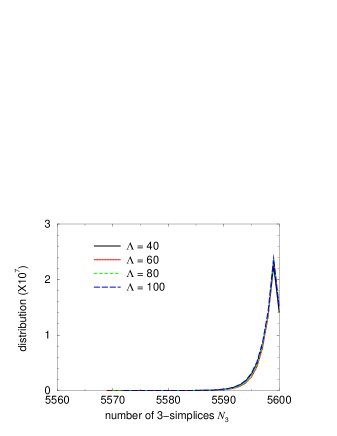
Figure 13: The $N_{3}$ distribution using the uniform measure $\prod_{i}dl_{i}$. The coupling constant $G$ is set to be $\infty$. Different curves correspond to different values of the cosmological constant ranging from ${\mit\Lambda}=40$ to ${\mit\Lambda}=100$. The maximum value of the horizontal axis is the upper cutoff of $N_{3}$.

Actually, we tried carrying out numerical calculations using the measure (32). In our numerical data with $G=\infty$ (strong coupling limit), however, the number of 3-simplices $N_{3}$ exhibits a clear tendency to diverge, even though we set large values of the cosmological constant ${\mit\Lambda}$, as shown in Fig. 13. Though the value of the cosmological constant varies from 40 to 100 in Fig. 13, the $N_{3}$ distribution is squeezed to the upper cutoff $N_{3}=5600$. Even if we choose larger values of the cutoff, the divergence behavior still appears in the same way. Hence, we cannot control the system (34) at all. From a viewpoint of statistical mechanics, one can interpret such a pathological behavior as follows. If the entropy bound (12) does not hold, the configuration entropy $W(N_{3})$ (given by eq. (9)) will dominate the system in the strong-coupling phase (high-temperature phase). In other words, lattice configurations with large $N_{3}$ will frequently appear owing to the large values of the entropy $W(N_{3})$, leading to the divergence of the lattice size. Actually, this is the case with our calculation using the uniform measure in Fig. 13. The large volume of the lattice diffeomorphisms will make large (presumably infinite) the entropy of such pathological configurations. In that sense the data of Fig. 13 indicates a piece of numerical evidence for the existence of the lattice symmetry.

At any rate, our calculation using the uniform measure cannot proceed further. Instead of the pathological measure, we should next try to use other measure that may break the diffeomorphism invariance at the quantum level.

5.1.2 Calculation using the scale-invariant measure

Next, we simulate the system (29) using the scale-invariant measure:

$$d\mu_{T}[l]=\prod_{i=1}^{N_{1}}\frac{\displaystyle dl_{i}}{\displaystyle l_{i}}\thinspace\delta_{T}(\Delta)\enspace.$$ (35)

Obviously, this measure is invariant under the local rescalings $l_{i}\to c_{i}l_{i}$ where $c_{i}$ are constants. In this case, the partition function is defined as

$$Z_{\mbox{\scriptsize DRC}}^{scale-inv}=\sum_{T}\int_{1}^{10}\prod_{i=1}^{N_{1}}dl_{i}\thinspace\exp\Bigl{(}-S[l,\thinspace T]\Bigr{)}\thinspace\delta_{T}(\Delta)\enspace,$$ (36)

where the action $S[l,\thinspace T]$ is of the form:

$$S[l,\thinspace T]=S_{\mbox{\scriptsize Regge}}[l,\thinspace T]+\sum_{i=1}^{N_{1}}\log l_{i}+\gamma(N_{3}-V)^{2}\enspace.$$ (37)

First of all, we measure the $N_{3}$ distribution, as shown in Fig. 14. One observes in the figure that $N_{3}$ distributes smoothly around the central value $V=5000$, in contrast to the uniform-measure case shown in Fig. 13. According to the numerical data of Fig. 14, one can naively expect that the exponential bound (12) will hold under this measure.

Figure 14: $N_{3}$ distribution using the scale-invariant measure $\prod_{i}dl_{i}/l_{i}$.

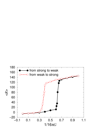
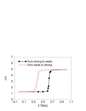
Figure 15: Hysteresis for the curvature $\langle R\rangle$ under the scale-invariant measure $\prod_{i}dl_{i}/l_{i}$. The solid line means the process from the strong to the weak coupling phase and the dashed vice versa.

Figure 16: Hysteresis for the average link-length $\langle l\rangle$ under the scale-invariant measure $\prod_{i}dl_{i}/l_{i}$. The solid line means the process from the strong to the weak coupling phase and the dashed vice versa.

In this case, we can obtain in principle any observables numerically, unlike the case of the uniform measure. Indeed, we measured the scalar curvature per volume, $\langle R\rangle$, as shown in Fig. 16. Evidently, this system has two phases, namely, the strong and the weak coupling phases; the solid line represents the cooling process from the strong coupling phase to the weak one, and the dotted its inverse. One can clearly observe a large hysteresis in Fig. 16, suggesting the first-order nature of the transition. It is consistent with results obtained in numerical studies of three-dimensional DT [43].

Next, we measured the average link-length $\langle l\rangle$ as shown in Fig. 16, where we observe another large hysteresis. In the strong-coupling phase, the strong gravitation prevents spacetime manifolds from extending widely, resulting in the small value of the length $\langle l\rangle$. In the weak-coupling phase, conversely, spacetime manifolds tend to stretch as widely as possible, resulting in spiky configurations. Such spikes of spacetime manifolds often appear also in the weak-coupling phase of quantum RC [13]. In this sense, our data of Fig. 16 is consistent with those obtained in the numerical studies of quantum RC.

Here we make a short remark on the statistics of our data. To get each point in Figs. 16 and 16, we accumulate 200 configurations, each of which is obtained at an interval of 800 sweeps. Statistical errors are also included in the figures, although they are too small to be visible.

5.2 Fractal structure of 3D pure gravity

We further investigate other structures of spacetime manifolds under the scale-invariant measure. Among them, a fractal structure based on a geodesic distance will be the most important, and its validity has been well established in two-dimensional DT [44]. Here we first explain the fractal structure and related issues for our purpose.

In the case of 3D gravity, the fractal structure is characterized by the surface area distribution (SAD) function $\rho(S,D)$ [45] and the fractal dimension $d_{f}$; their definitions will be given right now and closely related to each other. The SAD function is defined as follows [45]: (i) Let us consider a connected graph $\tilde{T}$ dual to a three-dimensional closed simplicial manifold $T$; (ii) The geodesic distance between two points in $\tilde{T}$ is defined as the minimum number of steps between the two points; (iii) We pick up a point $P$ in the graph $\tilde{T}$ (namely, a 3-simplex in $T$) and find all points that have a geodesic distance $D$ from the starting point $P$; (iv) The boundary manifold appearing in slicing $T$ at the geodesic distance $D$ consists of closed surfaces of various topologies, as shown in Fig. 17; (v) Then, the SAD function $\rho(S,\thinspace D)$ is defined as

$$\rho(S,\thinspace D)\equiv\mbox{the number of closed surfaces of area $S$ at the geodesic distance $D$}.$$ (38)

The fractal structure is encoded in the scaling behavior of the SAD function $\rho(S,D)$ with a scaling variable $x=S/D^{\alpha}$, where the exponent $\alpha$ has different values in different phases. $\rho(S,D)\times D^{\alpha}$ is expected to be a function only of $x$ in the scaling regions, and, therefore, it suggests a scaling law $S\sim D^{\alpha}$. As a result, the fractal dimension, $d_{f}$, of spacetime is determined as

$$d_{f}=\alpha+1\enspace.\vspace*{-0.1cm}$$ (39)

Intuitively, such a scaling means a self-similarity of ‘time slices’ that arise in cutting spacetime manifolds at different geodesic distances.

Incidentally, the scaling behavior of $\rho(S,\thinspace D)$ was observed numerically in three-dimensional DT [45], while its validity in studying quantum spacetime was first established in two-dimensional DT [44]. Moreover, a similar scaling behavior was reported also in four-dimensional DT [46].

Figure 17: Schematic picture of a three-dimensional fractal manifold that appears in the strong-coupling phase of DT. On the ‘time slice’ at a geodesic distance $D$ one can find many closed surfaces as the boundary. The fractal structure is revealed as the scaling property of the distribution of the closed surfaces at various geodesic distances.

According to the values of the gravitational constant $G$, we can classify the fractal structure into three regions: the strong-coupling, the critical, and the weak-coupling regions. An example of the fractal manifold with the scaling behavior is schematically depicted on Fig. 17, which occurs typically in the strong-coupling phase of three-dimensional DT. A closed surface of fairly large area appears only once at each ‘time slice’ $D$, which is the boundary of the so-called mother universe. Concurrently, there are many surfaces of small areas at each ‘time slice’ and they are boundaries of the baby universes. The boundaries of the mother and the baby universes consist of closed surfaces of various topologies.

Having reviewed the fractal structure of lattice gravity, we will devote our attention to the investigation of the structure in our hybrid model.

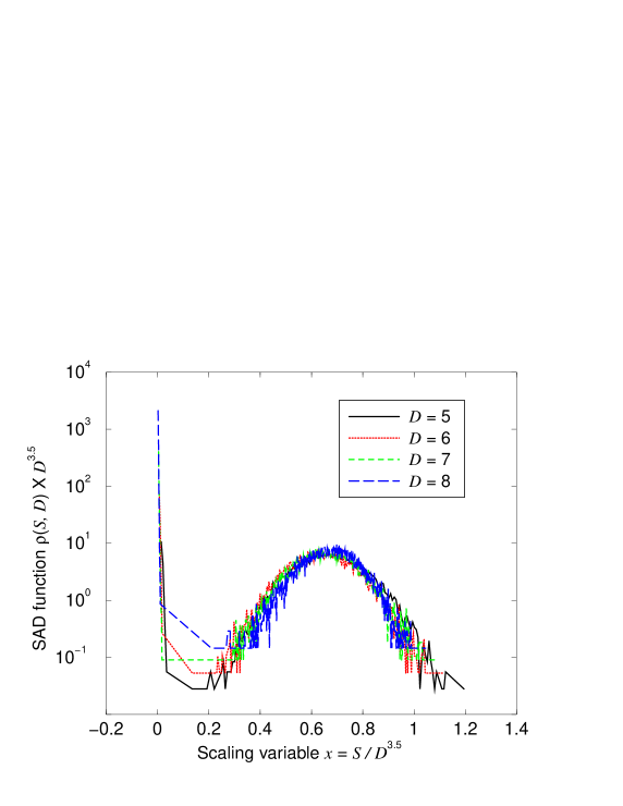
Figure 18: SAD function $\rho(S,\thinspace D)$ in the strong-coupling limit $G=\infty$ of 3D pure gravity based on DRC. The number of 3-simplices are almost fixed at about $N_{3}=5000$ and each link-length $l_{i}$ is integrated over a range $1<l_{i}<10$. Different curves correspond to different geodesic distances $D=5,6,7$ and 8. The scale-invariant measure $\prod_{i}dl_{i}/l_{i}$ is used.

Figure 19: Distributions of the Euler number $\chi$ in the strong-coupling limit $G=\infty$ of 3D pure gravity based on DRC. Different curves correspond to different geodesic distances $D=5,6,7$ and 8. The scale-invariant measure $\prod_{i}dl_{i}/l_{i}$ is used.

5.2.1 Fractal structure in the strong-coupling limit $G=\infty$

First, we measure the SAD function $\rho(S,\thinspace D)$ in the strong-coupling limit $G=\infty$ in DRC. Numerical data obtained is shown in Fig. 19, where the vertical axis means the SAD scaling function of the form $\rho(S,D)\times D^{3.5}$ and the horizontal a scaling variable $x=S/D^{3.5}$. The different curves show several data measured at different geodesic distances $D=5,6,7$ and 8. The boundary surface of the mother universe, which has the largest area among all boundaries, has a good scaling property with the scaling parameter $x=S/D^{3.5}$. Accordingly, the fractal dimension is obtained as $d_{f}=3.5+1=4.5$. One can clearly observe in Fig. 19 that the distribution of the mother universe has the Gaussian form. On the contrary, the distributions of the boundaries of the baby universes, whose areas are fairly smaller than that of the mother, do not exhibit a scaling behavior. In other words, it is impossible that the baby part scales in the same way as the mother does; such phenomenon of the existence of two scaling variables in a simplicial manifold typically appear also in three-dimensional DT [45].

Next, we measure the Euler number of the boundary surfaces. On each closed surface, the Euler number $\chi$ is defined in the usual way:

$$\chi\equiv n_{0}-n_{1}+n_{2}\enspace,$$ (40)

where $n_{k}$ mean the numbers of $k$-simplices $(k=0,1,2)$ on each boundary surface. Our numerical data of $\chi$ are shown in Fig. 19; obviously, surfaces with large negative $\chi$, exhibiting complicated topologies, are identified with the boundary of the mother universe. The distributions of the mother are in the shape of mountain (Gaussian) and, in contrast, those of the baby universes have a sharp peak at $\chi=2$. This result is consistent with that obtained in the strong-coupling phase of three-dimensional DT [45].

How can we draw a physical picture of this region? A plausible answer is a ‘confinement of spacetime’, into which all the volume of quantum spacetime is completely confined. Actually, the large fractal dimension, whose value is $d_{f}\sim 3.5+1$ in this limit, will prevent spacetime from extending, although the volume is not small. In addition, the large negative values of $\chi$ frequently appear in the distributions of the mother; this complexity of the topology reminds us of the spacetime foam.

5.2.2 Fractal structure in the critical region $G\sim G_{c}$

Second, we measure the SAD function and the Euler number distribution at $1/16\pi G=0.6$ in the critical region. Our numerical data are shown in Fig. 21 and Fig. 21. In Fig. 21, the vertical axis is the scaling function of the form $\rho(S,D)\times D^{2.3}$ and the horizontal the scaling variable $x=S/D^{2.3}$; the exponent 2.3 is vary small compared with the value obtained in the strong-coupling limit. Thus, we obtain a smaller fractal dimension $d_{f}=2.3+1=3.3$ in this region. In general, the smaller the fractal dimension becomes, the more widely the spacetime manifold extends.

Figure 20: SAD function $\rho(S,\thinspace D)$ at $1/16\pi G=0.6$ in the critical region of 3D pure gravity based on DRC. The number of 3-simplices are almost fixed at about $N_{3}=5000$ and each link-length $l_{i}$ is integrated over a range $1<l_{i}<10$. Different curves correspond to different geodesic distances $D=5,6,7$ and 8. The scale-invariant measure $\prod_{i}dl_{i}/l_{i}$ is used.

Figure 21: Distributions of the Euler number $\chi$ at $1/4\pi G=0.6$ in the critical region of 3D pure gravity based on DRC. Different curves corresponds to different geodesic distances $D=5,6,7$ and 8. The scale-invariant measure $\prod_{i}dl_{i}/l_{i}$ is used.

In this region, one cannot separate the contribution of the mother from that of the baby universes, because the scaling function $\rho(S,\thinspace D)$ distributes smoothly from small $x$ to large one. We have learned in two-dimensional DT that the distribution of the mother boundary is universal and, hence, it has the close connection with the continuum limit [44]. On the other hand, the distribution of the baby boundaries is non-universal; interestingly, the result shown in Fig. 21 is very similar to that obtained in two-dimensional DT [44], although the first-order nature of the transition indicates no continuum limit in our case.

Next, we measure the $\chi$ distributions of closed surfaces that appear in cutting the simplicial lattice at each geodesic distance. Our data is shown in Fig. 21, where the Euler number $\chi$ is measured at several distances. One can see that the $\chi$ distributions are fairly smoother than those of Fig. 19. As a result, we get a milder picture of spacetime in this region and the shape of the $\chi$ distribution is very similar to that obtained in three-dimensional DT [45].

5.2.3 Fractal structure in the weak-coupling phase $G<G_{c}$

Lastly, in the weak-coupling phase, we attempted to measure the same quantity $\rho(S,\thinspace D)$ in the same manner as in the strong-coupling and the critical regions. However, we cannot find any contributions from the mother universe in this phase and, what is worse, lattice configurations seem to be almost frozen, which have a lower fractal dimension; this phenomenon strongly suggests the spiky nature of spacetime in this phase, and such a spike is far from the usual notion of physical spacetime. As is well known with numerical studies of DT, this phase corresponds to an elongated branched-polymer with a small fractal dimension (for example, $d_{f}=2$) [45]. Similarly, such a spike has been observed also in Monte-Carlo studies of quantum RC [13].

6 Conclusions and discussion

We have proposed dynamical Regge calculus (DRC) as a hybrid model of simplicial quantum gravity. This model is intended to make physical degrees of freedom larger than those of quantum Regge calculus (RC) and dynamical triangulations (DT). Furthermore, the extended model of DRC gives the possibility of describing the topology-changing processes of Euclidean spacetime in a dynamical way, although there are some difficulties in simulating the processes numerically.

Algorithmically, the path integral for DRC (8) can be performed through the hybrid $(p,\thinspace q)$ moves, which are an extension of the ergodic $(p,\thinspace q)$ moves of DT. In particular, the lattice diffeomorphisms are generated by the invariance $(p,\thinspace q)$ moves. It is also an interesting problem that other constructive approaches to quantum gravity reproduce the same structure of the lattice diffeomorphisms as that of DRC, if one would believe the universality of field theory also in quantum gravity.

As an application of the lattice diffeomorphism, we tried a lattice-theoretic derivation of the black hole entropy. We identified the total number of quantum fluctuations around the event horizon with the black hole entropy; such hybrid moves that keep invariant the horizontal geometry play the important role. In order to avoid the divergence of the coefficient of the entropy, we required the lattice cutoff $l_{\rm min}$ to remain a finite value of order $O(\ell_{\rm P})$. The introduction of the minimal length seems to be consistent with a simple interpretation of the space-time uncertainty principle of string theory.

Moreover, we have carried out the numerical simulations of 3D pure gravity using the two kinds of the integration measures. In case of the uniform measure $\prod_{i}dl_{i}$ we observed the divergence behavior of the lattice size $N_{3}$ even though we chose the large values of the cosmological constant. This phenomenon indicates the exponential unboundedness for the entropy owing to the lattice diffeomorphisms. In this case DRC is not well-defined statistical-mechanically.

In case of the scale-invariant measure $\prod_{i}dl_{i}/l_{i}$, however, no pathological behavior occurred in our data. Indeed, we calculated the average curvature $\langle R\rangle$ and the average link-length $\langle l\rangle$; two pieces of large hysteresis were observed, indicating the existence of the first-order transition between the two phases. In the strong-coupling limit, spacetime manifolds are crumpled to a singular configuration with a large fractal dimension. Physically, such a crumpled space might suggest the existence of ‘confinement’, into which spacetime itself is confined. In addition, various topologies appear on time slices of ‘confined spacetime’. In the critical region, we have obtained the smooth SAD function, resulting in a milder picture of spacetime than in the strong-coupling limit. In this case spacetime looks a fractal manifold of lower fractal dimension. On the other hand, in the weak coupling phase simplicial configurations become spiky, and this phenomenon is essentially the same as that has been observed in the weak-coupling phase of quantum RC. Taking into account these theoretical and numerical studies, we conclude that DRC can reproduce the numerical results consistent with those of both DT and quantum RC in each region.

Our hybrid model of lattice quantum gravity offers a practical way of studying quantum black hole physics and the topology-change of Euclidean spacetime on the lattice. Incidentally, the close relation between 3D quantum gravity and quantization of the membrane theory [58] is an interesting theme in connection with string theory, though such an attempt generally gives rise to an instability problem [59]. Our chief concern is to investigate numerically the physics of strong-coupling quantum gravity within the framework of (extended) DRC.

Acknowledgments

I am grateful to K. Hamada for his detailed comments and suggestions. I would like to thank G. Kang for his useful comments on quantum black holes. I also wish to thank T. Yukawa and S. Horata for many useful discussions. Finally, I want to acknowledge valuable discussions with many members of Theory Division of KEK.

References

- [1] S. W. Hawking and G. F. R. Ellis, The large scale structure of space-time, Cambridge University Press (1973).
- [2] As texts of string theory, see, J. Polchinski, STRING THEORY I, II, Cambridge University Press (1998); M. B. Green, J. H. Schwartz and E. Witten, Superstring theory I, II, Cambridge University Press (1987).
- [3] For a review of loop quantum gravity, see, C. Rovelli, “Loop Quantum Gravity”, gr-qc/971008 (1997).
- [4] For a review of simplicial quantum gravity, see, F. David, “Simplicial Quantum Gravity and Random Lattices”, SACLAY preprint T93/028 (1993).
- [5] H. Hagura, “Dynamical Regge Calculus as Lattice Gravity”, Nucl. Phys. B (Proc. Suppl.) 94 (2001) 704.
- [6] H. Hagura, “Quantum geometry in dynamical Regge calculus”, Nucl. Phys. B (Proc. Suppl.) 106 (2002) 974.
- [7] D. Weingarten, Nucl. Phys. B210 (1982) 229.
-
[8]
F. David, Nucl. Phys. B257[FS14] (1985) 45.
V. A. Kazakov, Phys. Lett. B150 (1985) 282.
J. Ambjørn, B. Durhuus and J. Frhlich, Nucl. Phys. B257[FS14] (1985) 433; Nucl. Phys. B275[FS17] (1986) 161. - [9] For the basic theory of quantum Regge calculus, see, H. W. Hamber, in Critical Phenomena, Random Systems, Gauge Theories, Proceedings of the Les Houches Summer School 1984, eds. K. Osterwalder and R. Stora, North-Holland (1986).
- [10] H. W. Hamber and R. M. Williams, Nucl. Phys. B248 (1984) 392; B269 (1986) 712.
- [11] M. Roček and R. M. Williams, Z. Phys. C21 (1984) 371.
- [12] H. W. Hamber and R. M. Williams, Nucl. Phys. B487 (1997) 345.
- [13] H. W. Hamber and R. M. Williams, Phys. Rev. D47 (1993) 510.
- [14] M. Roček and R. M. Williams, Phys. Lett. 104B (1981) 31.
-
[15]
H. W. Hamber, Nucl. Phys. B20 (Proc. Supp.)
(1991) 728; Nucl. Phys. B400 (1993) 347.
H. W. Hamber and R. M. Williams, Nucl. Phys. B435 (1995) 361. - [16] J. Cheeger, W. Muller and R. Schrader, Commun. Math. Phys. 92 (1984) 405.
- [17] J. Bekenstein, Phys. Rev. D7 (1973) 2333; D9 (1974) 3292.
- [18] S. W. Hawking, Commun. Math. Phys. 43 (1975) 199; Phys. Rev. D13 (1976) 191.
- [19] S. W. Hawking, Nature (Physical Science), 248 (1974) 30.
- [20] J. Bekenstein, “DO WE UNDERSTAND BLACK HOLE ENTROPY ? ”, gr-qc/9409015.
- [21] L. Susskind and J. Uglum, “Black Hole Entropy in Canonical Quantum Gravity and Superstring Theory”, Phys. Rev. D50 (1994) 2700-2711, hep-th/9401070.
- [22] I. Moss, Phys. Rev. Lett. 69 (1992) 1852; M. Visser, Phys. Rev. D48 (1993) 583. R. Kallosh, T. Ortin and A. Peet, Phys. Rev. D47 (1993) 5400.
- [23] M. Srednicki, Phys. Rev. Lett.71 (1993) 666.
- [24] S. W. Hawking, “The path-integral approach to quantum gravity” in General Relativity: an Einstein Centenary Survey (ed. S. W. Hawking and W. Israel) Cambridge University Press, Cambridge (1979).
-
[25]
J. Distler and H. Kawai, Nucl. Phys. B321 (1989) 509.
V. G. Knizhnik, A. M. Polyaov and A. B. Zamolodchikov, Mod. Phys. Lett. A3 (1988) 819.
F. David, Mod. Phys. Lett. A3 (1988) 1651. -
[26]
D. J. Gross and A. A. Migdal, Nucl. Phys. B340
(1990) 333.
M. R. Dougras and S. H. Shenker, Nucl. Phys. B335 (1990) 635.
F. David, Nucl. Phys. B257[FS14] (1985) 45. - [27] B. De Witt, “Quantum Theory of Gravity: I. The Canonical Theory”, Phys. Rev. 160 (1967) 1113; “Quantum Theory of Gravity: II. The Manifestly Covariant Theory”, Phys. Rev. 162 (1967) 1195; “Quantum Theory of Gravity: III.Applications of the Covariant Theory”, Phys. Rev. 162 (1967) 1239.
- [28] G. W. Gibbons and S. W. Hawking, “Action integrals and partition function in quantum gravity”, Phys. Rev. D15 (1977) 2752; G. W. Gibbons, S. W. Hawking and M. J. Perry, “Path integrals and the indefiniteness of the gravitational action”, Nucl. Phys. B138 (1978) 141.
-
[29]
K. Hamada and F. Sugino, Nucl. Phys. B553
(1999) 283;
K. Hamada, Prog. Theor. Phys. 103 (2000) 1237; 105 (2001) 673. - [30] T. Regge, “General relativity without coordinate”, Nuovo Cimento 19 (1961) 558.
- [31] B. DeWitt, “The space time approach to quantum field theory”, in Relativity, Groups and Topology II, eds. K. Osterwalder and R. Stora, North-Holland (1984).
- [32] B. DeWitt, Phys. Rev. 160 (1967) 1113.
- [33] H. Römer and M. Zähringer, Class. Quant. Grav. 3 (1986) 897.
- [34] R. M. Williams, Nucl. Phys. [Proc. Suppl.] 57 (1997) 73, and references therein.
- [35] H. W. Hamber, Nucl. Phys. (Proc. Suppl.) 25A (1992) 150, and references therein.
- [36] For a brief review for both of classical and Regge calculus, see, R. M. Williams and P. A. Tuckey, Class. Quant. Grav. 9 (1992) 1409, and references therein.
- [37] H. W. Hamber and R. M. Williams, Nucl. Phys. B267 (1986) 482.
- [38] M. Gross and H. W. Hamber, Nucl. Phys. B364 (1991) 703.
- [39] H. W. Hamber, Int. J. Sup. Appl. 5 (1991) 84; Phys. Rev. D45 (1992) 507.
-
[40]
J. Alexander, Ann. Math. 31 (1930) 292.
M. Gross and S. Varsted, Nucl. Phys. B378 (1992) 367. - [41] U. Pachner, Europ. J. Phys. Combinatorics 12 (1991) 129.
- [42] S. Iso and H. Kawai, Int. J. Mod. Phys. A15 (2000) 651, hep-th/9903217.
-
[43]
D. V. Boulatov and A. Krzywicki,
Mod. Phys. Lett. A6 No.32 (1991) 3005;
J. Ambjørn and S. Varsted, Nucl. Phys. B377 (1992) 557. - [44] H. Kawai, N. Kawamoto, T. Mogami and Y. Watabiki, Phys. Lett. B306 (1993) 19.
-
[45]
H. Hagura, N. Tsuda and T. Yukawa, Phys. Lett. B418,
(1998) 273, hep-lat/9512016;
H. S. Egawa and N. Tsuda, Nucl. Phys. B (Proc. Suppl.) 63 (1998) 739, hep-lat/9711001 - [46] H. S. Egawa, T. Hotta, T. Izubuchi, N. Tsuda and T. Yukawa, Prog. Theor. Phys. 97 (1997) 539, hep-lat/9611028; H. S. Egawa, N. Tsuda and T. Yukawa, Nucl. Phys. B (Proc. Suppl.) 63 (1998) 736, hep-lat/9709099.
- [47] M. Fukuma, N. Ishibashi, H. Kawai and M. Ninomiya, Nucl. Phys. B427 (1994) 139, hep-th/9312175; M. Ikehara, N. Ishibashi, H. Kawai, T. Mogami, R. Nakayama and N. Sasakura, Phys. Rev. D50 (1994) 7467, hep-th/9406207
- [48] M. Lehto, H. B. Nielsen and M. Ninomiya, Nucl. Phys. B272 (1986) 213; B272 (1986) 228.
- [49] T. Yoneya, “String Theory and the Space-Time Uncertainty Principle”, Prog. Theor. Phys. 103 (2001) 1081, hep-th/0004074.
- [50] T. Yoneya, “Space-time uncertainty and noncommutativity in string theory”, Int. J. Mod. Phys. A16 (2001) 945 (Proceedings of the ‘Strings 2000’, Int. conf. Michigan Univ. 2000), hep-th/0010172.
- [51] R. Guida, K. Konishi and P. Provero, Mod. Phys. Lett. A6 (1991) 1487 and references therein.
- [52] J. A. Wheeler, “On the nature of Quantum Geometrodynamics”, Annals of Physics 2 (1957) 604; “Neutrinos, Gravitation and Geometry”, in Proceedings of the International School of Physics, “Enrico Fermi”, Course XI (Zanichelli, Bologna) (1960); Geometrodynamics (Academic Press, New York) (1962).
- [53] S. W. Hawking, “Spacetime foam”, Nucl. Phys. B144 (1978) 349.
- [54] T. Eguchi, P. B. Gilky and A. J. Hanson, “Gravitation, Gauge Theories and Differential Geometry”, Phys. Rep. 66 No. 6 (1980) 213.
- [55] S. Carlip, Phys. Rev. Lett. D51 (1995) 632.
- [56] Mu-In Park and Jeongwon Ho, Phys. Rev. Lett. 83 (1999) 5595.
- [57] M. Hotta, K. Sakai and T. Sakai, “Diffeomorphism on horizon as an asymptotic isometry of Schwarzschild black hole”, gr-qc/0011043, TU-606.
- [58] E. Bergshoeff, E. Sezgin and P. Townsent, Phys. Lett. B189 (1987) 75; Annals Phys. 185 (1988) 330.
-
[59]
B. de Witt, M. Luscher and H. Nicolai, Nucl. Phys. B320
(1989) 135.
B. de Witt, J. Hoppe and H. Nicolai, Nucl. Phys. B306 (1988) 545.