${\cal N}=(1,1)$ Super Yang–Mills on a (2+1) Dimensional Transverse Lattice with one Exact Supersymmetry

Motomichi Harada and Stephen Pinsky

Department of Physics
Ohio State University
Columbus OH 43210

We present a formulation of ${\cal N}=(1,1),$ Super Yang–Mills theory in 2+1 dimensions using a transverse lattice methods that exactly preserves one supersymmetry. First, using a Lagrangian approach we obtain a standard transverse lattice formulation of the Hamiltonian. We then show that the Hamiltonian also can be written discretely as the square of a supercharge and that this produces a different result. Problems associated with the discrete realization of the full supercharge algebra are discussed. Numerically we solve for the bound states of the theory in the large $N_{c}$ approximation and we find good convergence. We show that the massive fermion and boson bound states are all exactly degenerate and that the number of fermion and boson massless bound states are closely related. Also we find that this theory admits winding states in the transverse direction and that their masses vary inversely with the winding number.

1 Introduction

In 1976 Bardeen and Pearson [1, 2] proposed formulating a quantum field theory with a subset of the dimensions discretized on a spatial lattice. In the discrete spatial directions the theory was constructed to have discrete gauge invariance, identical to conventional lattice gauge theory. The remaining dimensions were then left to be treated by some other method. It is only in the last few years however that this idea has been fully exploited. There are two directions of research which rely on this idea that have been of some interest in recent years.

One research direction simply goes by the name “transverse lattice” [3]. For a review see [4]. This is a numerical method for solving quantum field theory. The name “transverse lattice” is somewhat deceptive because the method is actually the combination of several independent ideas, of which transverse lattice is only one. The other ingredient has to do with how one treats the longitudinal directions. There are analytical approaches to the longitudinal part of the problem designed to carefully treat the end points in momentum space [4], however they greatly limit the size of the basis one might use. The more common method goes by the name discrete light-cone quantization (DLCQ), and was itself proposed in 1985 by Brodsky and Pauli [5] as a numerical method to solve quantum field theories[6]. In DLCQ one quantizes the theory with a Hamiltonian $P^{-}=(P^{0}-P^{1})/\sqrt{2}$ that evolves the system in light-cone time $x^{+}=(x^{0}+x^{1})/\sqrt{2}$, uses the light-cone gauge $A^{+}=0$, and places the system in a light-cone spatial box. Thus, in this version of the transverse lattice approach one treats the longitudinal directions with a discrete momentum lattice and the transverse directions with a discrete spatial lattice.

The other research direction that uses the transverse lattice focuses on theories of extra dimensions. The directions that are put on a discrete lattice are dimensions that are beyond the normal 3+1 dimensions of conventional field theory. This approach suggested by Arkani-Hamed [7] and Hill [8] goes by the name “deconstruction”. Again the name is not very descriptive. The point is that when the extra dimensions are put on a discrete spatial lattice the extra dimensional field theory takes the form of a (3+1) dimensional theory where each of the fields carries additional labels corresponding to the structure of the extra dimensional space. If one is creative about this extra dimensional space this method can be a mechanism for constructing new and interesting field theories. Furthermore, since the theory is formulated as a field theory in 3+1 dimensions the renormalization is controllable.

With this very brief background we would like to suggest a slightly different direction. We have recently been studying a supersymmetric formulation of DLCQ which we call SDLCQ [9, 10, 11]. In many ways this approach is similar to DLCQ, however, it is formulated in such a way that the theory, which has discrete momenta and cutoffs in momentum space, is exactly supersymmetric. For a review, see [12]. Exact supersymmetry brings a number of very important numerical advantages to the method. In 1+1 and 2+1 [13, 14, 15] dimensions supersymmetric field theories are finite. We have also seen greatly improved convergence. In this paper we will attempt to formulate a (2+1)–dimensional ${\cal N}=1$ Super Yang–Mills (SYM) theory as a SDLCQ theory in 1+1 dimensions with a transverse spatial lattice in the one transverse direction. The challenge is to formulate it such that it is supersymmetric exactly at every order of the numerical approximation.

We will not be able to fully realize this goal. There are several fundamental problems that prevent complete success. In formulating this theory with gauge invariance in the one transverse dimension the gauge field is replaced by a complex unitary link field. Within the context of DLCQ this field is quantized as a linear complex field. This then disturbs the supersymmetry which usually requires the same number of fundamental fermion and boson fields. In some sense this is a restatement of the error we are making by treating a unitary field as a general complex field. There are simply too many boson degrees of freedom relative to the number of fermion degrees of freedom. Conventionally one adds a potential to a transverse lattice theory to enforce the unitarity of this complex boson field, but this is not possible within the context of an exactly supersymmetric theory. However, in the formulation of Gauss’s law on the transverse lattice, one finds that color conservation must be enforced at every lattice site. This greatly reduces the number of allowed boson degrees of freedom. It is unclear however if this constraint is sufficient to reduce the number of boson degrees of freedom to the number required by unitarity.

We will be able to partially formulate SDLCQ for this theory and write the Hamiltonian as the square of a supercharge. Previously we considered this situation in a different class of theories [16]. We will show that this produces a different and simpler discrete Hamiltonian than the standard lagrangian formulation. When we solve this theory using this partial formulation of SDLCQ we find that all of the massive states have exact fermion-boson degeneracy as required by full supersymmetry. Our partial SDLCQ does not require degeneracy between the massless fermion and boson states. We find however that they are nearly equal in number. The solution can be viewed as a unitary transformation from the constrained basis to an unconstrained basis and we see that in this new basis the number of fermion and boson degrees of freedom are very nearly equal. In effect, the partial supersymmetry and Gauss’s law are sufficient to approximately enforce the same symmetry in the spectrum that we would have obtained had we been able to enforce unitarity. Recently Dalley and Van de Sande [17, 18] have also pointed out the importance of Lorentz symmetry in enforcing the constraint of unitarity.

Since color is conserved at every transverse lattice site, there are two fundamentally different types of states. For one class of states the color flux winds around the space one or more times. We refer to these as cyclic states and to the other class of states as non-cyclic states. The spectrum for both classes of states are presented. For the cyclic states we present the spectrum as a function of the number of windings.

In Section 2, we present the standard lagrangian formulation of this theory of adjoint fermions and adjoint bosons. We show that Hamiltonian is sixth order in the field. In Section 3, we present the SDLCQ formulation which turns out to be only fourth order in the field. We show that there are two types of allowed states. One type loops the entire transverse space, and we study these state in Section 4. The states of the other type are localized, and we study these states in Section 5. In section 6 we discuss our conclusions and future work.

2 Transverse Lattice Model in 2+1 Dimensions

In this section we present the standard formulation of a transverse lattice model in 2+1 dimensions of an ${\cal N}=(1,1)$ supersymmetric $SU(N_{c})$ theory with both adjoint bosons and adjoint fermions in the large–$N_{c}$ limit.

We work in light cone coordinates so that $x^{\pm}\equiv(x^{0}\pm x^{1})/\sqrt{2}$. The metric is specified by $x^{\pm}=x_{\mp}$ and $x^{2}=-x_{2}$. Suppose that there are $N_{sites}$ sites in the transverse direction $x^{2}$ with lattice spacing $a$. With each site, $i$, we associate one gauge boson field $A_{\nu,i}(x^{\mu})$ and one spinor field $\Psi_{i}(x^{\mu})$, where $\nu,\mu=\pm$. $A_{\nu,i}$’s and $\Psi_{i}$’s are in the adjoint representation. The adjacent sites, say $i$ and $i+1$, are connected by what we call the link variables $M_{i}(x^{\mu})$ and $M_{i}^{{\dagger}}(x^{\mu})$, where $M_{i}(x^{\mu})$ stands for a link which goes from the $i$-th site to the $(i+1)$-th site and $M_{i}^{{\dagger}}(x^{\mu})$ for a link from the $(i+1)$-th to the $i$-th site. We impose the periodic condition on the transverse sites so that $A_{N_{sites}+1}=A_{1}$, $\Psi_{N_{sites}+1}=\Psi_{1}$, $M_{N_{sites}+1}=M_{1}$ and $M^{{\dagger}}_{N_{sites}+1}=M^{{\dagger}}_{1}$. Under the transverse gauge transformation [4] the fields transform as

$$gA_{i}^{\mu}\longrightarrow U_{i}gA_{i}^{\mu}U_{i}^{{\dagger}}-iU_{i}\partial^{\mu}U_{i}^{{\dagger}},\quad M_{i}\longrightarrow U_{i}M_{i}U_{i+1}^{{\dagger}},\quad\Psi_{i}\longrightarrow U_{i}\Psi_{i}U_{i}^{{\dagger}},$$ (1)

where $g$ is the coupling constant and $U_{i}\equiv U_{i}(x^{\mu})$ is a $N_{c}\times N_{c}$ unitary matrix. In all earlier work on the transverse lattice [4] $\Psi_{i}$ was in the fundamental representation.

The link variable can be written as

$$M_{i}(x^{\mu})=\exp\left(iagA_{i+1/2,\perp}(x^{\mu})\right),$$ (2)

where $A_{i,\perp}\equiv A_{i,2}$ is the transverse component of the gauge potential at site $i$ and as $a\to 0$ we can formally expand Eq. (2) in powers of $a$ as follows:

$$M_{i}(x^{\mu}) = 1+iagA_{i+1/2,\perp}(x^{\mu})-\frac{1}{2}\left(agA_{i+1/2,\perp}(x^{\mu})\right)^{2}+\ldots$$ (3)

$$= 1+iagA_{i,\perp}(x^{\mu})+\frac{a^{2}}{2}\left[ig\partial_{\perp}A_{i,\perp}(x^{\mu})-g^{2}\left(A_{i,\perp}(x^{\mu})\right)^{2}\right]+O(a^{3}).$$

In the limit $a\to 0$, with the substitution of the expansion Eq. (3) for $M_{i}$, we expect everything to coincide with its counterpart in continuum (2+1)–dimensional theory.

The discrete Lagrangian is then given by

$${\cal L} = {\rm tr}\Bigl{\{}-\frac{1}{4}F_{i}^{\mu\nu}F_{i,\mu\nu}+\frac{1}{2a^{2}g^{2}}\left(D_{\mu}M_{i}\right)\left(D^{\mu}M_{i}\right)^{{\dagger}}$$ (4)

$$+ \bar{\Psi}_{i}i\gamma^{\mu}D_{\mu}\Psi_{i}+\frac{i}{2a}\bar{\Psi}_{i}\gamma^{\perp}(M_{i}\Psi_{i+1}M_{i}^{{\dagger}}-M_{i-1}^{{\dagger}}\Psi_{i-1}M_{i-1})\Bigr{\}},$$

where the trace has been taken with respect to the color indices, $F_{i,\mu\nu}=\partial_{\mu}A_{i,\nu}-\partial_{\nu}A_{i,\mu}+ig[A_{i,\mu},A_{i,\nu}]$, $\mu$, $\nu$ = $\pm$ and $\gamma$’s are defined as follows

$$\gamma^{+}\equiv\frac{\gamma^{0}+\gamma^{1}}{\sqrt{2}}\equiv\frac{\sigma_{2}+i\sigma_{1}}{\sqrt{2}},\qquad\gamma^{-}\equiv\frac{\gamma^{0}-\gamma^{1}}{\sqrt{2}}\equiv\frac{\sigma_{2}-i\sigma_{1}}{\sqrt{2}},\qquad\gamma^{\perp}\equiv i\sigma_{3},$$

and the covariant derivative $D_{\mu}$ is defined as

$$D_{\mu}\Psi_{i} = \partial_{\mu}\Psi_{i}+ig[A_{i,\mu},\Psi_{i}],$$ (5)

$$D_{\mu}M_{i} = \partial_{\mu}M_{i}+igA_{i,\mu}M_{i}-igM_{i}A_{i+1,\mu}\ \stackrel{{\scriptstyle a\to 0}}{{\longrightarrow}}\ iagF_{\mu\perp},$$

$$(D^{\mu}M_{i})^{{\dagger}} = \partial^{\mu}M_{i}^{{\dagger}}-igM_{i}^{{\dagger}}A_{i}^{\mu}+igA_{i+1}^{\mu}M_{i}^{{\dagger}}\ \stackrel{{\scriptstyle a\to 0}}{{\longrightarrow}}\ iagF^{\mu\perp}.$$

Thus, in the limit $a\to 0$ one finds, as expected,

$${\cal L}\ \stackrel{{\scriptstyle a\to 0}}{{\longrightarrow}}\ {\rm tr}\left(-\frac{1}{4}F^{\alpha\beta}F_{\alpha\beta}+i\Psi i\gamma^{\alpha}D_{\alpha}\Psi\right),$$

where $\alpha$, $\beta=\pm,\perp$. Of course the form of this Lagrangian is slightly different from that in Ref. [4] since the fermions are in the adjoint representation. This Lagrangian is hermitian and invariant under the transformation in Eq. (1) as one would expect.

The following Euler-Lagrange equations in the light cone gauge, $A_{i,-}=0$, are constraint equations.

$$\partial_{-}^{2}A_{i}^{-}\equiv gJ_{i}^{+},\qquad\partial_{-}\chi_{i}=\frac{1}{2\sqrt{2}a}(M_{i}\psi_{i+1}M_{i}^{{\dagger}}-M_{i-1}^{{\dagger}}\psi_{i-1}M_{i-1})\ \stackrel{{\scriptstyle a\to 0}}{{\longrightarrow}}\ \frac{1}{\sqrt{2}}D_{\perp}\psi,$$ (6)

where

$$J_{i}^{+} \equiv \frac{i}{2g^{2}a^{2}}(M_{i}\stackrel{{\scriptstyle\leftrightarrow}}{{\partial}}_{-}M_{i}^{{\dagger}}+M_{i-1}^{{\dagger}}\stackrel{{\scriptstyle\leftrightarrow}}{{\partial}}_{-}M_{i-1})+2\psi_{i}\psi_{i}$$ (7)

$$\stackrel{{\scriptstyle a\to 0}}{{\longrightarrow}} \ i[A_{\perp},\partial_{-}A_{\perp}]+\frac{1}{g}\partial_{-}\partial_{\perp}A_{\perp}+2\psi\psi,$$ (8)

$$\Psi_{i} \equiv \frac{1}{2^{1/4}}\left(\begin{array}[]{c}\psi_{i}\\ \chi_{i}\end{array}\right).$$ (11)

Since these equations only involve the spatial derivative we can solve them for $A_{i}^{-}$ and $\chi_{i}$, respectively. Thus the dynamical field degrees of freedom are $M_{i}$, $M_{i}^{{\dagger}}$ and $\psi_{i}$.

The first of the equations in Eq. (6) gives a constraint on physical states $|phys\rangle$, since the zero mode of $J^{+}_{i}$ acting on any physical state must vanish,

$$\stackrel{{\scriptstyle 0}}{{J^{+}_{i}}}|phys\rangle=\int dx^{-}J^{+}_{i}(x^{\mu})|phys\rangle=0\quad{\rm for}\ {\rm any}\ i.$$ (12)

The physical states must be color singlet at each site.

It is straightforward to derive $P^{\pm}\equiv\int dx^{-}T^{+\pm}$, where $T^{\mu\nu}$ is the stress-energy tensor. We have

$$P^{+} = a\sum_{i=1}^{N_{sites}}\int dx^{-}{\rm tr}\left(\frac{1}{a^{2}g^{2}}\partial_{-}M_{i}^{{\dagger}}\partial_{-}M_{i}+i\psi_{i}\partial_{-}\psi_{i}\right)$$ (13)

$$\stackrel{{\scriptstyle a\to 0}}{{\longrightarrow}} \int dx^{-}dx^{\perp}{\rm tr}\left((\partial_{-}A_{\perp})^{2}+i\psi\partial_{-}\psi\right),$$ (14)

and

$$P^{-} = a\sum_{i=1}^{N_{sites}}\int dx^{-}{\rm tr}\left[\frac{1}{2}(\partial_{-}A_{i}^{-})^{2}+i\chi_{i}\partial_{-}\chi_{i}\right]$$ (15)

$$= a\sum_{i=1}^{N_{sites}}\int dx^{-}{\rm tr}\Bigl{[}-\frac{g^{2}}{2}J^{+}_{i}\frac{1}{\partial_{-}^{2}}J^{+}_{i}$$

$$-\frac{i}{8a^{2}}(M_{i}\psi_{i+1}M_{i}^{{\dagger}}-M_{i-1}^{{\dagger}}\psi_{i-1}M_{i-1})\frac{1}{\partial_{-}}(M_{i}\psi_{i+1}M_{i}^{{\dagger}}-M_{i-1}^{{\dagger}}\psi_{i-1}M_{i-1})\Bigr{]}$$

$$\stackrel{{\scriptstyle a\to 0}}{{\longrightarrow}} \int dx^{-}dx^{\perp}{\rm tr}\Bigl{[}-\frac{g^{2}}{2}J^{+}\frac{1}{\partial_{-}^{2}}J^{+}-\frac{i}{2}D_{\perp}\psi\frac{1}{\partial_{-}}D_{\perp}\psi\Bigr{]}.$$ (16)

When one quantizes the dynamical fields, unitarity of $M_{i}$ is lost and $M_{i}$ becomes an $N_{c}\times N_{c}$ imaginary matrix [3, 4]. Some have suggested the addition of an effective potential $V(M_{i})$ to force $M_{i}$ to be a unitary matrix in the limit $a\to 0$ [1, 2, 4]. We will approach this issue using supersymmetry.

Having linearized $M_{i}$, we can expand $M_{i}$ and $\psi_{i}$ in their Fourier modes as follows; at $x^{+}=0$

$$M_{i,rs}(x^{-}) = \frac{ag}{\sqrt{2\pi}}\int_{0}^{\infty}\frac{dk^{+}}{\sqrt{k^{+}}}(d_{i,rs}(k^{+}){\rm e}^{-ik^{+}x^{-}}+a_{i,sr}^{{\dagger}}(k^{+}){\rm e}^{ik^{+}x^{-}}),$$ (17)

$$\psi_{i,rs}(x^{-}) = \frac{1}{2\sqrt{\pi}}\int_{0}^{\infty}dk^{+}(b_{i,rs}(k^{+}){\rm e}^{-ik^{+}x^{-}}+b_{i,sr}^{{\dagger}}(k^{+}){\rm e}^{ik^{+}x^{-}}),$$ (18)

where $r,s$ indicate the color indices, $a_{i,sr}^{{\dagger}}(k^{+})$ creates a link variable with momentum $k^{+}$ which carries color $r$ at site $i$ to $s$ at site $(i+1)$, $d^{{\dagger}}_{i,sr}(k^{+})$ creates a link with $k^{+}$ which carries color $r$ at site $(i+1)$ to $s$ at site $i$ and $b^{{\dagger}}_{i,sr}$ creates a fermion at the $i$-site which carries color $r$ to $s$. Quantizing at $x^{+}=0$ we have

$$[M_{i,rs}(x^{-}),\pi_{M_{j},pq}(y^{-})]=[M_{i,rs}^{{\dagger}}(x^{-}),\pi_{M^{{\dagger}}_{j},pq}(y^{-})]$$

$$=\{\psi_{i,rs}(x^{-}),\pi_{\psi_{j},pq}(y^{-})\}=\frac{i}{2}\delta(x^{-}-y^{-})\frac{\delta_{ij}}{a}\delta_{rp}\delta_{sq}.$$ (19)

Note that we divided $\delta_{ij}$ by $a$ because $\delta_{ij}/a\to\delta(x^{\perp}-y^{\perp})$as $a\to 0$. The conjugate momentum are

$$\pi_{M_{i}}=\frac{1}{2a^{2}g^{2}}\partial_{-}M_{i}^{{\dagger}},\quad\pi_{M_{i}^{{\dagger}}}=\frac{1}{2a^{2}g^{2}}\partial_{-}M_{i},\quad\pi_{\psi_{i}}=i\psi_{i}.$$

Thus we must have

$$[M_{i,rs}(x^{-}),\partial_{-y}M^{{\dagger}}_{j,pq}(y^{-})] = [M_{i,rs}^{{\dagger}}(x^{-}),\partial_{-y}M_{j,pq}(y^{-})]=ia^{2}g^{2}\delta(x^{-}-y^{-})\frac{\delta_{ij}}{a}\delta_{rp}\delta_{sq},$$

$$\{\psi_{i,rs}(x^{-}),\psi_{j,pq}(y^{-})\} = \frac{1}{2}\delta(x^{-}-y^{-})\frac{\delta_{ij}}{a}\delta_{rp}\delta_{sq}.$$ (20)

Then, one can easily see that these commutation relations are satisfied when $a$’s, $d$’s and $b$’s satisfy the following:

$$[a_{i,rs}(k^{+}),a^{{\dagger}}_{j,pq}(p^{+})]=[d_{i,rs}(k^{+}),d^{{\dagger}}_{j,pq}(p^{+})]=\{b_{i,rs}(k^{+}),b^{{\dagger}}_{j,pq}(p^{+})\}=\delta(k^{+}-p^{+})\frac{\delta_{ij}}{a}\delta_{rp}\delta_{sq},$$ (21)

with others all being zero. Physical states can be generated by acting on the Fock vacuum $|0\rangle$ with these $a^{{\dagger}}$’s, $d^{{\dagger}}$ and $b^{{\dagger}}$’s in such a manner that the constraint Eq. (12) is satisfied.

Let us complete this section by discussing the physical constraint (12) in more detail. The states are all constructed in the large–$N_{c}$ limit, and therefore we need only consider single–trace states. In order for a state to be color singlet at each site, each color index has to be contracted at the same site. As an example consider a state represented by $|phys\ 1\rangle\equiv d^{{\dagger}}_{i,rs}(k_{1}^{+})a^{{\dagger}}_{i,sr}(k^{+}_{2})|0\rangle$. For this state the color $r$ at site $i$ is carried by $a^{{\dagger}}_{i}$ to $s$ at site $(i+1)$ and then brought back by $d^{{\dagger}}_{i}$ to $r$ at site $i$. The color $r$ is contracted at site $i$ only and the color $s$ at site $(i+1)$ only. Therefore, this is a physical state satisfying Eq. (12). A picture to visualize this case is shown in Fig. 1a.

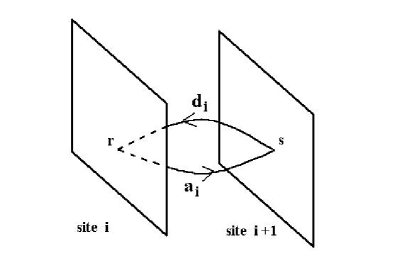
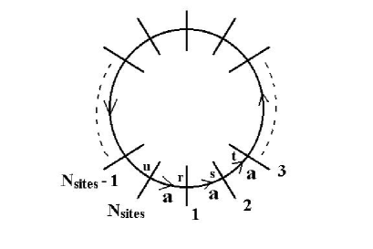
(a)	(b)

Figure 1: (a)The color charge for the state $|phys\ 1\rangle\equiv d^{{\dagger}}_{i,rs}(k_{1}^{+})a^{{\dagger}}_{i,sr}(k^{+}_{2})|0\rangle$. The planes represent the color space. $a_{i}$ carries color $r$ at site $i$ to $s$ at site $i+1$ and $d_{i}$ carries it back to $r$ at site $i$. (b) The color for the state $|phys\ 2\rangle\equiv a^{{\dagger}}_{i+N_{sites}-1,ru}(k^{+}_{N_{sites}})\cdots a^{{\dagger}}_{i+1,ts}(k^{+}_{2})\cdot a^{{\dagger}}_{i,sr}(k^{+}_{1})|0\rangle$. The lines which intersect a circle represent the color planes at sites. The color goes all the way around the transverse lattice.

One also needs to be careful with operator ordering. One can show that the state $d^{{\dagger}}_{i,rs}(k^{+}_{1})a^{{\dagger}}_{i,st}(k^{+}_{2})b^{{\dagger}}_{i,tr}(k^{+}_{3})|0\rangle$ is physical, while the state $b^{{\dagger}}_{i,rs}(k^{+}_{1})a^{{\dagger}}_{i,st}(k^{+}_{2})d^{{\dagger}}_{i,tr}(k^{+}_{3})|0\rangle$ is unphysical.

We should, however, note that a true physical state be summed over all the transverse sites since we have discrete translational symmetry in the transverse direction. That is, for example, the states $d^{{\dagger}}_{1,rs}(k_{1}^{+})a^{{\dagger}}_{1,sr}(k^{+}_{2})|0\rangle$ and $d^{{\dagger}}_{2,rs}(k_{1}^{+})a^{{\dagger}}_{2,sr}(k^{+}_{2})|0\rangle$ are the same up to a phase factor given by $\exp(iP^{\perp}a)$. We set the phase factor to one since we take physical state to have $P^{\perp}=0$. The physical state $|phys\ 1\rangle$ is in fact $\sum_{i=1}^{N_{sites}}d^{{\dagger}}_{i,rs}(k_{1}^{+})a^{{\dagger}}_{i,sr}(k^{+}_{2})|0\rangle$ with the appropriate normalization constant. From a computational point of view this is a great simplification because we can drop the site index i from the representation.

Periodic conditions on the fields, allow for physical states of the form $|phys\ 2\rangle\equiv\sum_{i}a^{{\dagger}}_{i+N_{sites}-1,ru}(k^{+}_{N_{sites}})\cdots a^{{\dagger}}_{i+1,ts}(k^{+}_{2})\cdot a^{{\dagger}}_{i,sr}(k^{+}_{1})|0\rangle$. The color for this state is carried around the transverse lattice, as shown in Fig. 1b. We will refer to these states as cyclic states. The states where the color flux does not go all the way around the transverse lattice we will refer to as non-cyclic states. We characterize states by what we call the winding number defined by $W=n/N_{sites}$, where $n\equiv\sum_{i}(a_{i}^{{\dagger}}a_{i}-d^{{\dagger}}_{i}d_{i})$. Using the Eguchi–Kawai[19] reduction which applies in the large–$N_{c}$ limit we can always take $N_{sites}=1$. The winding number simply gives us the excess number of $a^{{\dagger}}$ over $d^{{\dagger}}$ in a state. We use the winding number to classify states since the winding number is a good quantum number commuting with $P^{-}_{SDLCQ}$. In the language of the winding number the non-cyclic states are those states with $W=0$ and cyclic states have non-zero $W$.

It is straight forward to show that $|phys\rangle$ satisfies Eq. (12) but $|unphys\rangle$ does not using

$$(\stackrel{{\scriptstyle 0}}{{J^{+}_{i}}})_{pq} = \int dk^{+}a^{{\dagger}}_{i,rp}(k^{+})a_{i,rq}(k^{+})-d_{i,pr}(k^{+})d^{{\dagger}}_{i,qr}(k^{+})-a_{i-1,pr}(k^{+})a^{{\dagger}}_{i-1,qr}(k^{+})$$ (22)

$$+d^{{\dagger}}_{i-1,rp}(k^{+})d_{i-1,rq}(k^{+})+b_{i,pr}(k^{+})b^{{\dagger}}_{i,qr}(k^{+})+b^{{\dagger}}_{i,rp}(k^{+})b_{i,rq}(k^{+}).$$

Diagrammatically, one can say that at every point in color space at any site one has to have either no lines or two lines, one of which goes into and the other of which comes out of the point, so that the color indices are contracted at the same site.

3 SDLCQ of the Transverse Lattice Model

The transverse lattice formulation of ${\cal N}=1$ SYM theory in 2+1 dimension presented in the previous section has several undesirable features. The supersymmetric structure of the theory is completely hidden and the resulting Hamiltonian is $6^{th}$ order in the fields. From the numerical point of view a $6^{th}$ order interaction makes the theory considerably more difficult to solve. Also the underlying (2+1)–dimensional supersymmetric Hamiltonian is only $4^{th}$ order making this discrete formulation of the theory very different than the underlying theory. There can, of course, be many discrete formulations that correspond to the same continuum theory and it is therefore desirable to search for a better one. In the spirt of SDLCQ we will attempt a discrete formulation based on the underlying super algebra of this theory,

$$\{Q^{\pm},Q^{\pm}\}=2\sqrt{2}P^{\pm},\quad\{Q^{+},Q^{-}\}=2P^{\perp}.$$ (23)

In this effort there are some fundamental limits to how far one can go. As we discussed in the previous section the physical states of this theory must conserve color at every point on the transverse lattice. Experience with other supersymmetric theories indicates that each term in $Q^{+}$ has to be either the product of one $M_{i}$ and one $\psi_{i}$ or of one $M_{i}^{{\dagger}}$ and one $\psi_{i}$ therefore $Q^{+}$ is unphysical, by which we mean that $Q^{+}$ transforms a physical state into an unphysical one, so that $\langle phys|Q^{+}|phys\rangle=0$. While this is not a theorem, it seems very difficult to have any other structure since in light cone quantization $P^{+}$ is a kinematic operator and therefore independent of the coupling. There appears to be no way to make a physical $P^{+}$ from $Q^{+}$. We will use $P^{+}$ as given in Eq. (13) in what follows. Similarly, we are not able to generally construct $P^{\perp}$ from $Q^{+}$ and $Q^{-}$. In fact $P^{\perp}$ is unphysical in our formalism, leading to $\langle phys|P^{\perp}|phys\rangle=0$. Formally we will work in the frame where total $P^{\perp}$ is zero, so it would appear consistent with this result. However, $P^{\perp}=0$ was a choice and a non-zero value is equally valid and not consistent with the matrix element.

Despite these difficulties we find a physical $Q^{-}$ which gives us $P^{-}_{SDLCQ}\stackrel{{\scriptstyle a\to 0}}{{\longrightarrow}}P^{-}_{cont}$. The expression for $Q^{-}$ and $P^{-}_{SDLCQ}$ are, respectively,

$$Q^{-} = 2^{3/4}g\cdot a\sum_{i=1}^{N_{sites}}\int dx^{-}{\rm tr}(J_{i}^{+}\partial^{-1}_{-}\psi_{i})$$

$$\stackrel{{\scriptstyle a\to 0}}{{\longrightarrow}} 2^{3/4}\int dx^{-}dx^{\perp}{\rm tr}\left[\partial_{\perp}A^{\perp}\psi+g\left(i[A^{\perp},\partial_{-}A^{\perp}]+2\psi\psi\right)\partial^{-1}_{-}\psi\right],$$

$$P^{-}_{SDLCQ} \equiv \frac{\{Q^{-},Q^{-}\}}{2\sqrt{2}}$$ (25)

$$= a\sum_{i}\int dx^{-}{\rm tr}[-\frac{g^{2}}{2}J_{i}^{+}\frac{1}{\partial_{-}^{2}}J_{i}^{+}-\frac{i}{2a^{2}}(\psi_{i+1}M^{{\dagger}}_{i}-M_{i}^{{\dagger}}\psi_{i})\partial^{-1}(M_{i}\psi_{i+1}-\psi_{i}M_{i})]$$

$$\stackrel{{\scriptstyle a\to 0}}{{\longrightarrow}} \int dx^{-}dx^{\perp}{\rm tr}\Bigl{[}-\frac{g^{2}}{2}J^{+}\frac{1}{\partial_{-}^{2}}J^{+}-\frac{i}{2}D_{\perp}\psi\frac{1}{\partial_{-}}D_{\perp}\psi\Bigr{]}\equiv 2\sqrt{2}P^{-}_{cont}.$$

Notice that this Hamiltonian is only $4^{th}$ order in the fields. Furthermore, one can check that this $Q^{-}$ commutes with $P^{+}$ obtained from ${\cal L}$; $[Q^{-},P^{+}]=0$. Thus, it follows that,

$$\langle phys|[Q^{-},M^{2}]|phys\rangle=\langle phys|[Q^{-},2P^{+}P^{-}_{SDLCQ}]|phys\rangle=0$$ (26)

in our SDLCQ formalism, where $M^{2}\equiv 2P^{+}P^{-}_{SDLCQ}-(P^{\perp})^{2}$. The fact that the Hamiltonian is the square of a supercharge will guarantee the usual supersymmetric degeneracy of the massive spectrum, and our numerical solutions will substantiate this. Unfortunately one needs a $Q^{+}$ to guarantee the degeneracy of the massless bound states.

The expression for $Q^{-}$ is

$$:Q^{-}: = \frac{i2^{-1/4}ag}{\sqrt{\pi}}\sum_{i}\int dk_{1}\ dk_{2}\ dk_{3}\delta(k_{1}+k_{2}-k_{3})\Bigl{[}$$ (27)

$$\frac{k_{2}-k_{1}}{k_{3}\sqrt{k_{1}k_{2}}}(-b_{i}^{{\dagger}}d_{i}a_{i}+d_{i}^{{\dagger}}a_{i}^{{\dagger}}b_{i}-b^{{\dagger}}_{i}a_{i-1}d_{i-1}+a^{{\dagger}}_{i-1}d_{i-1}^{{\dagger}}b_{i})$$

$$+\frac{k_{2}+k_{3}}{k_{1}\sqrt{k_{2}k_{3}}}(-d_{i}^{{\dagger}}b_{i}d_{i}+b_{i}^{{\dagger}}d_{i}^{{\dagger}}d_{i}-a^{{\dagger}}_{i-1}b_{i}a_{i-1}+b^{{\dagger}}_{i}a_{i-1}^{{\dagger}}a_{i-1})$$

$$+\frac{k_{3}+k_{1}}{k_{2}\sqrt{k_{3}k_{1}}}(a_{i}^{{\dagger}}a_{i}b_{i}-a_{i}^{{\dagger}}b_{i}^{{\dagger}}a_{i}+d^{{\dagger}}_{i-1}d_{i-1}b_{i}-d^{{\dagger}}_{i-1}b_{i}^{{\dagger}}d_{i-1})$$

$$+\left(\frac{1}{k_{1}}+\frac{1}{k_{2}}-\frac{1}{k_{3}}\right)(b^{{\dagger}}_{i}b^{{\dagger}}_{i}b_{i}+b^{{\dagger}}_{i}b_{i}b_{i})\Bigr{]},$$

where $k^{+}\equiv k$, $a^{{\dagger}}a\equiv{\rm Tr}(a^{{\dagger}}(k_{1})a(k_{2}))$, $a^{{\dagger}}aa\equiv{\rm Tr}(a^{{\dagger}}(k_{3})a(k_{1})a(k_{2}))$, $a^{{\dagger}}a^{{\dagger}}a\equiv{\rm Tr}(a^{{\dagger}}(k_{1})a^{{\dagger}}(k_{2})a(k_{3}))$. Notice that from this explicit expression for $Q^{-}$ it is clear that cyclic states do not get mixed with non-cyclic states under $Q^{-}$, as advertised at the end of the second section. Notice also that the winding number introduced in the last section evidently commutes with $Q^{-}$ and, thus, with $P^{-}_{SDLCQ}$.

Now we are in a position to solve the eigenvalue problem $2P^{+}P^{-}_{SDLCQ}|phys\rangle=m^{2}|phys\rangle$. We impose the periodicity condition on $M_{i}$, $M^{{\dagger}}_{i}$ and $\psi_{i}$ in the $x^{-}$ direction giving a discrete spectrum for $k^{+}$:

$$k^{+}=\frac{\pi}{L}n\quad(n=1,2,\ldots.),\qquad\int_{0}^{\infty}dk^{+}\rightarrow\frac{\pi}{L}\sum_{n=1}^{\infty}.$$

We impose a cut-off on the total longitudinal momentum $P^{+}$ i.e. $P^{+}=\pi K/L$, where $K$ is an integer also known as the ‘harmonic resolution’, which indicates the coarseness of our numerical results. For a fixed $P^{+}$ i.e. a fixed $K$, the number of partons in a state is limited up to the maximum, that is $K$, so that the total number of Fock states is finite, and, therefore, we have reduced the infinite dimensional eigenvalue problem to a finite dimensional one. We should note here that since the matrix $\langle phys|P_{SDLCQ}^{-}|phys\rangle$ to be diagonalized does not depend on $N_{sites}$, the resulting spectrum does not depend on $N_{sites}$, either. This means there is no need to keep the site index of operators even in numerical calculations; the sum over all the sites is implicitly understood and when one needs to restore the site indices for some reason, one should do so in such a way that physical constraint (12) is satisfied. Henceforth we will suppress the sum and the site indices, unless otherwise noted.

For this initial study of the transverse lattice we only consider resolution up to $K=8$ for $W=0,1$ states and up to $K=W+5$ and $K=W+4$ for states with $|W|=2,3$ and $|W|=4,5$, respectively. We were able to handle these calculations with our SDLCQ Mathematica code. In the following two sections we will give the numerical results for the cyclic $(W\neq 0)$ states and non-cyclic $(W=0)$ states separately.

4 Numerical Results for the Cyclic $(W\neq 0)$ States

For the cyclic states, it is easy to see that $K\geq|W|$. In fact if $K=|W|$, only two states are possible and both are bosonic they are ${\rm tr}(a^{{\dagger}}_{i+N_{sites}-1}\cdots a^{{\dagger}}_{i+1}a^{{\dagger}}_{i})|0\rangle$ and ${\rm tr}(d^{{\dagger}}_{i}d^{{\dagger}}_{i+1}\cdots d^{{\dagger}}_{i+N_{sites}-1})|0\rangle$, Therefore we will focus on $K>|W|$. Since there is an exact $Z_{2}$ symmetry between positive $W$ and negative $W$, it suffices to consider the case where $W$ is positive.

K–W 1 2 3 4 5 6 7 $W$  massive fermion or boson states 1 0 1 5 18 62 208 706 2 0 2 10 38 138 492 3 0 3 17 68 268 1023 4 0 4 24 110 470 5 0 5 33 166 770 massless boson states 1 0 1 1 3 3 8 8 2 1 2 2 5 5 12 3 1 2 2 5 5 15 4 1 2 2 6 6 5 1 2 2 6 6 massless fermion states 1 1 1 2 2 4 4 9 2 1 1 2 2 5 5 3 1 1 2 2 5 5 4 1 1 2 2 6 5 1 1 2 2 6

Table 1: Number of massive and massless cyclic eigenstates.

Table 1 shows the number of eigenstates with different $K$ and $W$ for various types of states. Since the spectrum starts at $K=W$, it is natural to take $K-W$ as the independent variable. Therefore we tabulate the number of eigenstates with $W$ and $K-W$ rather than $W$ and $K$ and we plotted $m^{2}$ as a function $1/(K-W)$ rather than in $1/K$

The massive degenerate fermion and boson states are related by $Q^{-}$ $|F\rangle\equiv|B\rangle$. The same is not true of massless states. There is no direct connection through $Q^{-}$ between massless fermionic states and massless bosonic states, leading to a supersymmetry breaking for massless states. Nevertheless, Table 1 shows that we have the exact supersymmetry for massless states when $K-|W|=2n-1$ for $n=2,\ldots$. The boson state with $W=1$ is anomalous since ${\rm tr}(a^{{\dagger}})=0$ in our formulation.

Also notice that there is a jump in the number of massless states with every increment by two in $K$. This seems to be the case because we need to increase $K$ by two to allow for the addition of an operator like $d_{i}^{{\dagger}}(1)a_{i}^{{\dagger}}(1)$, so as to make a new physical massless state. The requirement that we add a pair of bosons relates back to the Gauss’s law constraint. We see here that two bosons are behaving as a single boson. This is additional evidence that Gauss’s law and supersymmetry are working together to restrict the number of effective boson degrees of freedom. It is particularly reassuring to see this effect in the massless bound states since it is in this sector where breaking of the supersymmetric spectrum occurs. We also notice some other interesting properties of our massless states. We find that the Fock states that occur in bosonic massless states have no fermionic operators, whereas the Fock states that occur in fermionic massless states have only one fermionic operator, which seems to explain the relative shift between the number of massless fermion and bosons.

In Fig. 2(a) and (b) we give plots of $m^{2}$ for two low–energy states as a function of $1/(K-W)$ and extract $m^{2}_{\infty}$ as a $K\to\infty$ limit of the linear fit. We identify an energy eigenstate with different $K$’s according to dominant Fock states. Looking at both bosonic and fermionic counterpart also helps distinguish states. We present two states we could easily identify. For the state in (a) the dominate fock component has the form $b^{{\dagger}}(n)a^{{\dagger}}(1)\cdots a^{{\dagger}}(1)b^{{\dagger}}(1)+b^{{\dagger}}(1)a^{{\dagger}}(1)\cdots a^{{\dagger}}(1)b^{{\dagger}}(n)$ while the state in (b) has the dominate component $b^{{\dagger}}(n)a^{{\dagger}}(1)\cdots a^{{\dagger}}(1)b^{{\dagger}}(1)-b^{{\dagger}}(1)a^{{\dagger}}(1)\cdots a^{{\dagger}}(1)b^{{\dagger}}(n)$.

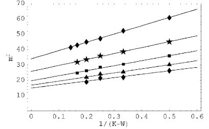
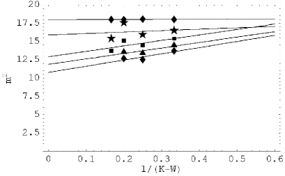
(a)	(b)

Figure 2: Plots of $m^{2}$ in units of $\frac{N_{c}g^{2}}{\pi a}$ of low energy cyclic states versus $1/(K-W)$ with a linear fit for W=1(top diamond), 2(star), 3(square), 4(triangle), 5(bottom diamond) (a) state A and, (b) state B.

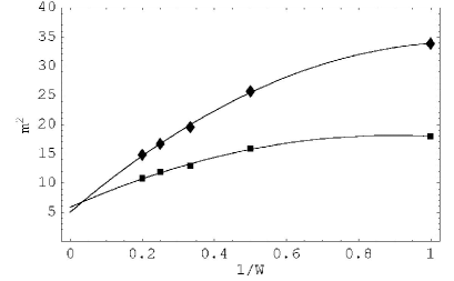
Figure 3: Plots of $K\to\infty$ limit of $m^{2}$ in units of $\frac{N_{c}g^{2}}{\pi a}$ of low energy cyclic states versus $1/W$ with a quadratic fit to the data. The diamond correspond state A box and squares correspond to the state B in Fig. 2

In Fig. 3 we present $m^{2}_{\infty}$, obtained in Fig.2(a) and (b), as a function of $1/W$ and show a quadratic fit to the data. $m^{2}$ is fit very well with a quadratic fit in $1/W$ In 2+1 dimensions the Hamiltonian has the form $P^{-}=a+bk_{\perp}+ck_{\perp}^{2}$. With periodic boundary conditions $k_{\perp}=n_{\perp}\pi/L$ and for cyclical states $L=aW$. Thus we expect that $m^{2}$ is a function of the winding number to be of the form $m^{2}=A+B/W+C/W^{2}$, as we find.

This behavior is consistent with the unique properties of SYM theories that we have seen in previous SDLCQ calculations [9, 10]. We have seen that as we increase $K$ we discover new lower mass bound states. Most of the partons in these long states appear to gluons. Supersymmetric theories like to have light states with long strings of gluons. We call these states with long strings of gluons, stringy states. In the full SDLCQ solution of the ${\cal N}=1$ SYM theory in 1+1 dimensions we found that these stringy states have an accumulation point at zero mass. In the full SDLCQ calculation of ${\cal N}=1$ SYM theory in 2+1 dimensions we have seen stringy states as well, but we have not seen evidence for an accumulation point. We will need to go to higher resolution to make a similar analysis for this theory.

5 Numerical Results for the Non-Cyclic $(W=0)$ States

Let us now discuss numerical results for the non-cyclic states. Table 2 shows the number of mass eigenstates of massive bosons or fermions, massless bosons, and massless fermions with different $K$.

$K=$ 3 4 5 6 7 8 massive fermion or boson states 2 6 22 72 238 792 massless boson states 1 3 3 7 7 17 massless fermion states 1 1 3 3 7 7

Table 2: Number of massive and massless non-cyclic eigenstates

From the table we see once again that there are some differences in the number of the massless bosonic and fermionic states and the same dependence on $K$ that we saw for the cyclic states. The reason for this behavior is the same as in the case of the cyclic states.

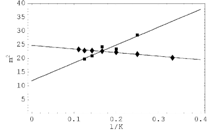
Figure 4: Plots of $m^{2}$ of low–energy non-cyclic states against $1/K$ with a linear fit in units of $\frac{N_{c}g^{2}}{\pi a}$.

In Fig. 4 we show two states whose boson states with a large two partons component. These states appear at the lowest resolution and are the easiest to follow and identify as a function of the resolution $K$. The boson bound state denoted by diamonds is composed primarily of two fermions, $b^{{\dagger}}b^{{\dagger}}$, while the boson bound state denoted by squares is composed primarily of two bosons, $d^{{\dagger}}a^{{\dagger}}$. Again, we see stringy states which appear as we go to higher $K$ with more partons in their dominate Fock state component.

We were able go up to $K=8$ without making any approximations to the Fock basis, so some of our bound states contained as many as eight partons. However, for $K=9$ we have truncated the number of partons at 6. We were able to justify this approximation at $K=9$ for this state by comparing the truncated results with the exact result at $K=8$. However we were not able to make this approximation for the state denoted by squares.

6 Discussion

We have presented a formulation of ${\cal N}=(1,1)$ SYM in 2+1 dimensions where the transverse dimension is discretized on a spatial lattice while the longitudinal dimension $x^{-}$ is discretized on a momentum lattice. Both $x^{-}$ and $x^{\perp}$ are compact. We are able to retain some of the technology of SDLCQ, since this numerical approximation retains one exact supersymmetry. In particular we are able to write the Hamiltonian as the square of a supercharge. Thus there is sufficient supersymmetry in this formulation to ensure that divergences that appear in this theory are automatically canceled. Furthermore we show that this formulation leads to a fundamentally different and simpler discrete Hamiltonian than the standard Lagrangian approach to the transverse lattice. Since we only have one exact supersymmetry, only the massive fermion and boson bound states in our solution are exactly degenerate. We need an additional supersymmetry to require that the numbers of massless bosons and massless fermions be the same.

As in all transverse lattice approaches, the transverse gauge field is replaced by a complex unitary field, and transverse gauge invariance is maintained. When this complex unitary field is quantized as a general complex linear field, the number of degrees of freedom in the transverse gauge field is improperly represented. In a conventional transverse lattice calculation one tries to dynamically enforce the proper number of degrees of freedom by adding a potential that is minimized by the unitarity constraint. We conjecture that this is not necessary here. Gauss’s law requires that color be conserved at every transverse lattice site. This greatly restrict the allowed boson Fock states that can be part of the physical set of basis states and plays an important role in the structure of all bound states. We assert that the combination of the Gauss’s law constraint and the one exact supersymmetric are sufficient to approximately enforce the full supersymmetry.

To further support this conjecture we note that in the massless spectrum the number of states changes when we change the resolution by two units indicating that it effectively requires two partons to represent one true degree of freedom. We view solving the theory as a unitary transformation from the constrained basis to a basis free of constraints and very nearly fully supersymmetric.

We should note that this conjecture can not be general since we know of one supersymmetric theory in 1+1 dimensions where the degrees of freedom at the parton level are all fermions [21]. In this model one has to fix the coupling to be a particular value for this miracle to occur. Generally in a supersymmetric theory the coupling is a free parameter. Nevertheless this example provides of word of caution with regard to our assertion.

We found two classes of bound states, cyclic and non-cyclic. The cyclic bound states have color flux that is wrapped completely around the compact transverse space. We were able to isolate two sequences of such states. Each sequence corresponds to a given state with a different number of wrappings. As a function of the winding number W the masses have the form $m^{2}=A+B/W+C/W^{2}$. In the non-cyclic sector we find stringy states as we have in previous SDLCQ calculations. We find good convergence for the bound states we present as a function of K.

Finally we would like to note that the symmetries of this approach and those of Cohn, Kaplan, Katz and Unsal (CKKU)[22] appear to be similar. The formulations are totally different, and these authors consider a two–dimensional discrete spacial lattice as well as extended supersymmetry. Nevertheless there are some similarities. As we have noted several times we have color conservation at each lattice site, thus the symmetry group is $U(N_{c})^{N_{sites}}$ similar to CKKU. We have enforced translation invariance for this discrete lattice with $N_{sites}$ sites; therefore, there is a $Z_{N_{sites}}$ symmetry similar to one found by CKKU for their two dimensional lattice. Finally, in this theory there is an orientation symmetry for the trace which is a $Z_{2}$ symmetry also similar to CKKU. In addition CKKU have some $U(1)$ symmetries which we seem to be missing. This may be related to the fundamentally different way chiral symmetry is treated on the light cone[6]. Another similarity appears to be the relation between the number of supersymmetries and the number of fermions on a site. Both approaches have one fermion on a site and one supersymmetry.

Numerically this calculation was done using our Mathematica code on a Linux workstation. This was very convenient for our first attempt at a supersymmetric formulation of a transverse lattice problem. The trade off is that it limits significantly how far we can go in resolution and in the number of sites. Our current $C++$ code can be modified to handle this problem and will allow a significantly increased resolution. We should also be able to handle the problem of two transverse dimensions with this code. These appear to be fruitful directions for future research.

References

- [1] W. A. Bardeen and R. B. Pearson, Phys. Rev. D14, 547 (1976)
- [2] W. A. Bardeen, R. B. Pearson and E. Rabinocici, Phys. Rev. D 21, 1037 (1980)
- [3] S. Dalley and B. van de Sande, Phys. Rev. D 56, 7917 (1997); Phys. Rev. D 59, 065008 (1999); Phys. Rev. Lett. 82, 1088 (1999); Phys. Rev. D 62, 014507 (2000); Phys. Rev. D 63, 076004 (2001); Phys. Rev. D 64, 036006 (2001).
- [4] M. Burkardt and S. Dalley, Prog. Part. Nucl. Phys. 48, 317 (2002). arXiv:hep-th/0112007.
- [5] H.-C. Pauli and S.J. Brodsky, Phys. Rev. D 32, 1993 (1985); 32, 2001 (1985).
- [6] S.J. Brodsky, H.-C. Pauli, and S.S. Pinsky, Phys. Rep. 301, 299 (1998), arXiv:hep-ph/9705477.
- [7] N. Arkani-Hamed, A. G. Cohen, and H. Georgi, Phys. Rev. Lett.86, 4757 (2001) arXiv:hep-th/0104005
- [8] C. T. Hill, S. Pokorski and J. Wang, Phys. Rev. D 64, 105005 (2001) arXiv:hep-th/0104035.
- [9] F. Antonuccio, O. Lunin, and S. S. Pinsky, Phys. Lett. B 429, 327 (1998), arXiv:hep-th/9803027.
- [10] F. Antonuccio, O. Lunin, and S. Pinsky, Phys. Rev. D 58, 085009 (1998), arXiv:hep-th/9803170.
- [11] F. Antonuccio, O. Lunin, S. Pinsky , and S. Tsujimaru, Phys. Rev. D 60, 115006 (1999), arXiv:hep-th/9811254.
- [12] O. Lunin and S. Pinsky, AIP Conf. Proc. 494, 140 (1999), arXiv:hep-th/9910222.
- [13] F. Antonuccio, O. Lunin and S. Pinsky, Phys. Rev. D 59, 085001 (1999), arXiv:hep-th/9811083.
- [14] P. Haney, J. R. Hiller, O. Lunin, S. Pinsky and U. Trittmann, Phys. Rev. D 62, 075002 (2000), arXiv:hep-th/9911243.
- [15] J. R. Hiller, S. Pinsky and U. Trittmann, Phys. Rev. D 64, 105027 (2001), arXiv:hep-th/0106193
- [16] O. Lunin and S. Pinsky, Phys. Rev. D 63, 045019 (2001) [arXiv:hep-th/0005282].
- [17] S. Dalley, Phys. Rev. D 64, 036006 (2001) [arXiv:hep-ph/0101318].
- [18] S. Dalley and B. van de Sande, arXiv:hep-ph/0212086.
- [19] T. Eguchi and H. Kawai, Phys. Rev. Lett. 48 (1983) 1063
- [20] Y. Matsumura, N. Sakai, and T. Sakai, Phys. Rev. D 52, 2446 (1995).
- [21] D. Kutasov, Phys. Rev. D48 (1993) 4980, arXiv:hep–th/9306013
- [22] A. Cohen, D. Kaplan, E. Katz and M. Unsal, “Supersymmetry on a Euclidean Space Time Lattice 1” arXiv:hep-lat/0302017.