Chiral Anomalies in the Reduced (or Matrix) Model

Abstract

We show that, with an appropriate choice of a Dirac operator, there is a remnant of chiral anomalies in the reduced model in which there is no coordinate dependences of the gauge field. This result is obtained by exploring a topological nature of chiral anomalies associated to Ginsparg-Wilson-type lattice Dirac operators.

1 Introduction

We already had several talks concerning new ideas on a treatment of chiral fermions in lattice gauge theory in this workshop.[2] The essence of these new ideas can be summarized in a simple relation which is called the Ginsparg-Wilson relation. In this talk, I present another kind of application of these new ideas in lattice gauge theory.

2 Axial Anomaly with the Ginsparg-Wilson Relation

The Ginsparg-Wilson relation[3] of $d$-dimensional lattice Dirac operator reads

$$\gamma_{d+1}D+D\gamma_{d+1}=D\gamma_{d+1}D.$$ (1)

Here $\gamma_{d+1}$ is the $d$-dimensional analogue of $\gamma_{5}$ and I set the lattice spacing unity $a=1$ for notational simplicity. An important consequence of this relation is a topological property of the axial anomaly, which is defined by

$$q(x)\equiv\mathop{\rm tr}\nolimits\gamma_{d+1}\left[1-{1\over 2}D(x,x)\right]{\buildrel a\to 0\over{\rightarrow}}{1\over 2}\partial_{\mu}\langle\overline{\psi}\gamma_{\mu}\gamma_{d+1}\psi(x)\rangle.$$ (2)

From the algebraic relation (1) and the “$\gamma_{5}$-hermiticity” $D^{\dagger}=\gamma_{d+1}D\gamma_{d+1}$, one can show the “index relation”[4] on a lattice $\mathit{\Gamma}$

$$Q\equiv\sum_{x\in\mathit{\Gamma}}q(x)=\mathop{\rm Tr}\nolimits\gamma_{d+1}\left(1-{1\over 2}D\right)=n_{+}-n_{-},$$ (3)

where $n_{\pm}$ is a number of zero-modes of $\gamma_{d+1}D$ with $\pm$ chirality. The integer $Q$ therefore provides a topological characterization of a gauge field configuration, even on a finite-size lattice.

We take Neuberger’s overlap Dirac operator[5] as a definite example of $D$:

$$D=1-{A\over\sqrt{A^{\dagger}A}},\quad A=1-D_{\rm w},\quad D_{\rm w}={1\over 2}[\gamma_{\mu}(\nabla_{\mu}^{*}+\nabla_{\mu})-\nabla_{\mu}^{*}\nabla_{\mu}].$$ (4)

In this construction, covariant difference operators are defined by

$$\nabla_{\mu}=U_{\mu}(x)T_{\mu}-1,\quad\nabla_{\mu}^{*}=1-U_{\mu}(x-\hat{\mu})^{\dagger}T_{\mu}^{\dagger},$$ (5)

where $T_{\mu}$ is the shift operator: $T_{\mu}\psi(x)=\psi(x+\hat{\mu})$.

Now, assuming that the combination $Q$ (3) gives a non-trivial value $n_{+}-n_{-}\neq 0$ (this turns to be actually the case), the index relation (3) implies that the overlap operator $D$ cannot be a smooth function of the gauge field in general: The space of lattice gauge fields is arc-wise connected and the integer $Q$ cannot “jump” unless $D$ becomes singular at certain points (see Fig. 1).

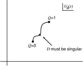
Figure 1: The overlap Dirac operator $D$ must be singular at a certain point on a path from $Q=0$ to $Q=1$.

To avoid these singularities, some restriction on gauge field configurations has to be imposed. For the overlap-Dirac operator, a sufficient condition for the well-defined-ness of $D$ is known as “admissibility”[6]

$$\|1-U_{\mu}(x)U_{\nu}(x+\hat{\mu})U_{\mu}(x+\hat{\nu})^{\dagger}U_{\nu}(x)^{\dagger}\|<\epsilon,$$ (6)

for all plaquettes, where $\|\mathcal{O}\|=\sup_{v\neq 0}\|\mathcal{O}v\|/\|v\|$. This condition divides (otherwise arcwise-connected) space of lattice gauge fields into many topological sectors (see Fig. 2).

Figure 2: After imposing the admissibility, topological sectors emerge.

With a lattice Dirac operator which obeys the Ginsparg-Wilson relation, the topological structure of gauge theory naturally emerges in this way. It is interesting that this picture works even with finite lattice sizes and with finite lattice spacings, namely for a system of finite degrees of freedom.

Furthermore, when the gauge group is $\mathop{\rm{}U}(1)$, the topological nature of the axial anomaly allows a non-perturbative cohomological analysis. Using the facts that $q(x)$ is a gauge invariant local pseudoscalar field which satisfies $\sum_{x\in\mathit{\Gamma}}\delta q(x)=0$, one can show that the most general form of $q(x)$ is given by[7]

$$q(x) = \gamma\epsilon_{\mu_{1}\nu_{1}\cdots\mu_{d/2}\nu_{d/2}}F_{\mu_{1}\nu_{1}}(x)F_{\mu_{2}\nu_{2}}(x+\hat{\mu}_{1}+\hat{\nu}_{1})\cdots$$ (7)

$$\quad\times F_{\mu_{d/2}\nu_{d/2}}(x+\hat{\mu}_{1}+\hat{\nu}_{1}+\cdots+\hat{\mu}_{d/2-1}+\hat{\nu}_{d/2-1})$$

$$+\partial_{\mu}^{*}k_{\mu}(x),$$

where $F_{\mu\nu}(x)={1\over i}\ln U_{\mu}(x)U_{\nu}(x+\hat{\mu})U_{\mu}(x+\hat{\nu})^{\dagger}U_{\nu}(x)^{\dagger}$ and $k_{\mu}(x)$ is a certain gauge invariant local periodic current on $\mathit{\Gamma}$. This is the first example (to my knowledge) that one can see an explicit structure of the axial anomaly in a system with finite UV and IR cutoffs. This non-perturbative information was fully utilized in a manifestly gauge invariant lattice formulation of $\mathop{\rm{}U}(1)$ chiral gauge theories.[8] The coefficient $\gamma$ can be obtained by a matching with the classical continuum limit as $\gamma=(-1)^{d/2}/[(4\pi)^{d/2}(d/2)!]$.[9]

The general argument (3) tells that $Q$ is an integer. One can see this fact more directly when the gauge group is $\mathop{\rm{}U}(1)$. In this case, gauge fields which satisfies the admissibility (6) can be completely classified as[8]

$$U_{\mu}(x)=\Lambda(x)V_{\mu}^{[m]}(x)U_{\mu}^{[w]}(x)e^{iA_{\mu}^{\rm T}}(x)\Lambda(x+\hat{\mu})^{-1},$$ (8)

where $\Lambda(x)$ is the gauge degrees of freedom and $U_{\mu}^{[w]}(x)$ carries the Polyakov line, $\prod_{s=0}^{L-1}U_{\mu}^{[w]}(s\hat{\mu})=w_{\mu}\in\mathop{\rm{}U}(1)$. The part $V_{\mu}^{[m]}(x)$ has a constant field strength $F_{\mu\nu}(x)=2\pi m_{\mu\nu}/L^{2}$, where $m_{\mu\nu}\in{\mathbb{Z}}$, and $A_{\mu}^{\rm T}(x)$ represents gauge invariant local fluctuations. Then, by using eqs. (3) and (7), we have

$$Q={(-1)^{d/2}\over 2^{d/2}(d/2)!}\,\epsilon_{\mu_{1}\nu_{1}\cdots\mu_{d/2}\nu_{d/2}}m_{\mu_{1}\nu_{1}}m_{\mu_{2}\nu_{2}}\cdots m_{\mu_{d/2}\nu_{d/2}},$$ (9)

for $\mathop{\rm{}U}(1)$ theories; this is manifestly an integer.

Here we present an application of above ideas to the reduced model.

3 Reduced model and the $\mathop{\rm{}U}(1)$ embedding

The $\mathop{\rm{}U}(N)$ reduced model is defined by a zero-volume limit of $\mathop{\rm{}U}(N)$ lattice gauge theory, $U_{\mu}(x)\in\mathop{\rm{}U}(N)\to U_{\mu}\in\mathop{\rm{}U}(N)$. This kind of reduction appears in the Eguchi-Kawai reduction of the large $N$ QCD[10] and in the compact version of IKKT IIB matrix model.[11] Here we concentrate on the fermion sector in the reduced model: $\psi(x)\to\psi\in\hbox{fundamental rep.\ of $\mathop{\rm{}U}(N)$}$. According to above prescriptions, the covariant derivative for the reduced fermion field would be read as

$$\nabla_{\mu}=U_{\mu}(x)T_{\mu}-1\to U_{\mu}-1.$$ (10)

In the reduced model, one would expect that there is no anomaly as $\mathop{\rm tr}\nolimits F\cdots F(x)\to\mathop{\rm tr}\nolimits A\cdots A\equiv 0$. We will show that in an appropriate framework there exists some remnant of chiral anomalies even in this zero-dimensional field theory.

To show this, we first assume $N=L^{d}$, where $L$ is an integer. Then we can identify an index of the fundamental representation $n$ and a site $x$ on a lattice $\mathit{\Gamma}$ of the size $L$, $x=(x_{1},\ldots,x_{d})$, by $n(x)=1+x_{d}+Lx_{d-1}+\cdots+L^{d-1}x_{1}$. With this identification, the $N\times N$ matrix $T_{\mu}=1\otimes\cdots\otimes 1\otimes X\otimes 1\otimes\cdots 1$, where the factor $X$

$$X=\pmatrix{0&1&&\cr&\ddots&\ddots&\cr&&\ddots&1\cr 1&&&0\cr},$$ (11)

appears in the $\mu$-th entry, realizes the shift on the lattice (while preserving the periodic boundary condition) as $T_{\mu}f_{n(x)}=f_{n(x+\hat{\mu})}$.

So next we assume that the reduced gauge field has the following particular form

$$U_{\mu}=u_{\mu}T_{\mu},$$ (12)

where $u_{\mu}$ is a diagonal matrix

$$u_{\mu}=\pmatrix{(u_{\mu})_{1}&&\cr&\ddots&\cr&&(u_{\mu})_{N}\cr}.$$ (13)

Note $(u_{\mu})_{n}\in\mathop{\rm{}U}(1)$. Then the covariant derivative in the reduced model takes the form

$$\nabla_{\mu}=U_{\mu}-1=u_{\mu}T_{\mu}-1.$$ (14)

By comparing this with eq. (5), we realize that the fermion sector of the reduced model with $U_{\mu}=u_{\mu}T_{\mu}$ is completely equivalent to that of the conventional $\mathop{\rm{}U}(1)$ lattice gauge theory. The $\mathop{\rm{}U}(1)$ gauge field in the latter is diagonal elements of the matrix $u_{\mu}$. In this sense, we call eq. (12) $\mathop{\rm{}U}(1)$ embedding.

An interesting property of the $\mathop{\rm{}U}(1)$ embedding is that the plaquette is identical for both pictures:

$$U_{\mu}U_{\nu}U_{\mu}^{\dagger}U_{\nu}^{\dagger} = u_{\mu}(T_{\mu}u_{\nu}T_{\mu}^{\dagger})(T_{\nu}u_{\mu}^{\dagger}T_{\nu}^{\dagger})u_{\nu}^{\dagger}$$ (15)

$$= u_{\mu}(x)u_{\nu}(x+\hat{\mu})u_{\mu}(x+\hat{\nu})^{*}u_{\nu}(x)^{*},$$

due to the relation $(T_{\mu}fT_{\mu}^{\dagger})_{m(x)n(y)}=f_{m(x+\hat{\mu})n(y+\hat{\mu})}$ which holds for a diagonal matrix $f$. Also the trace on the side of the reduced model is simply written by a lattice summation, $\mathop{\rm tr}\nolimits f=\sum_{x\in\mathit{\Gamma}}f(x,x)$. In this way, we can switch between matrix- and lattice-pictures.

4 Vector-like reduced model and the topological charge

Following the proposal of Kiskis, Narayanan and Neuberger,[13] we use the overlap-Dirac operator in the reduced model. It is defined by the construction (4) with the substitution (10) and $\nabla_{\mu}^{*}=1-U_{\mu}^{\dagger}$. As they demonstrated for $d=2$ and $4$ by using a somewhat different idea, this framework provides a well-defined topological charge for reduced gauge fields. To make the overlap-Dirac operator well-defined, one imposes the admissibility $\|1-U_{\mu}U_{\nu}U_{\mu}^{\dagger}U_{\nu}^{\dagger}\|<\epsilon$ on reduced gauge fields. Then the axial anomaly (or the topological charge) in the reduced model, $Q=\mathop{\rm tr}\nolimits\gamma_{d+1}(1-D/2)$, provides a well-defined topological characterization of the reduced gauge field. Recall Fig. 2.

By further using the $\mathop{\rm{}U}(1)$ embedding (12), we can use the above matrix-lattice correspondence. The crucial point is that the admissibility is common for both pictures as eq. (15) shows. So we can literally copy results in Sec. 2! In this way, we immediately find that $Q$ in the reduced model is given by eq. (9). Note that the integers $m_{\mu\nu}$ this time parameterize a form of matrices $U_{\mu}$. See ref. [1]. By this way, we see that there exist reduced gauge fields which have non-trivial topological charges.

5 Chiral gauge reduced model and an obstruction

By using Ginsparg-Wilson-type Dirac operator, one can formulate chiral gauge reduced model, along the line of ref. [8]. This formulation is equivalent to the overlap [14]. A complexity of this formulation is, however, the fermion integration measure has an ambiguity in its phase and one has to fix this ambiguity somehow. After imposing the admissibility, the space of gauge fields may have a complicated topology (see Fig. 2) and then it is not obvious whether the phase can be chosen as a single-valued function on this space. This problem can be formulated in terms of a $\mathop{\rm{}U}(1)$ fiber bundle associated to a phase of the fermion measure.[15, 8] If and only if this bundle is trivial, one can define a single-valued expectation value in the fermion sector. One of measures of a non-triviality of the bundle is the first Chern number (the monopole charge) $\mathcal{I}$ defined for closed 2 dimensional surfaces in the space of admissible gauge fields. If we have $\mathcal{I}\neq 0$ for a certain surface, the bundle cannot be trivial and a Weyl fermion cannot be consistently formulated.

By using the $\mathop{\rm{}U}(1)$ embedding and a cohomological analysis of Lüscher’s topological field in $d+2$ dim.,[8] we found there exists a 2-torus such that $\mathcal{I}\neq 0$. Space does not permit a detailed presentation. See ref. [1]. This shows that a Weyl fermion in the fundamental rep. of $\mathop{\rm{}U}(N)$ in the reduced model cannot be consistently formulated within this framework. We regard this as a remnant of the gauge anomaly of the original gauge theory. A generalization of this result to other gauge-group representations is under study.

References

- [1] Y. Kikukawa and H. Suzuki, J. High Energy Phys. 0209, 032 (2002) [hep-lat/0207009].
- [2] T. W. Chiu, these proceedings. Y. Kikukawa, these proceedings.
- [3] P. H. Ginsparg and K. G. Wilson, Phys. Rev. D25, 2649 (1982).
- [4] P. Hasenfratz, V. Laliena and F. Niedermayer, Phys. Lett. B427, 125 (1998) [hep-lat/9801021].
- [5] H. Neuberger, Phys. Lett. B417, 141 (1998) [hep-lat/9707022]; Phys. Lett. B427, 353 (1998) [hep-lat/9801031].
- [6] P. Hernández, K. Jansen and M. Lüscher, Nucl. Phys. B552, 363 (1999) [hep-lat/9808010]. H. Neuberger, Phys. Rev. D61, 085015 (2000) [hep-lat/9911004].
- [7] M. Lüscher, Nucl. Phys. B538, 515 (1999) [hep-lat/9808021]. T. Fujiwara, H. Suzuki and K. Wu, Nucl. Phys. B569, 643 (2000) [hep-lat/9906015]; Phys. Lett. B463, 63 (1999) [hep-lat/9906016]. H. Igarashi, K. Okuyama and H. Suzuki, Nucl. Phys. B644, 383 (2002) [hep-lat/0206003].
- [8] M. Lüscher, Nucl. Phys. B549, 295 (1999) [hep-lat/9811032]; Nucl. Phys. B568, 162 (2000) [hep-lat/9904009].
- [9] Y. Kikukawa and A. Yamada, Phys. Lett. B448, 265 (1999) [hep-lat/9806013]. K. Fujikawa, Nucl. Phys. B546, 480 (1999) [hep-th/9811235]. D. H. Adams, Annals Phys. 296, 131 (2002) [hep-lat/9812003]; J. Math. Phys. 42, 5522 (2001) [hep-lat/0009026]. H. Suzuki, Prog. Theor. Phys. 102, 141 (1999) [hep-th/9812019]. T.-W. Chiu and T.-H. Hsieh, hep-lat/9901011. T. Fujiwara, K. Nagao and H. Suzuki, J. High Energy Phys. 0209, 025 (2002) [hep-lat/0208057].
- [10] T. Eguchi and H. Kawai, Phys. Rev. Lett. 48, 1063 (1982). G. Bhanot, U. M. Heller and H. Neuberger, Phys. Lett. B113, 47 (1982).
- [11] N. Kitsunezaki and J. Nishimura, Nucl. Phys. B526, 351 (1998) [hep-th/9707162]. T. Tada and A. Tsuchiya, Prog. Theor. Phys. 103, 1069 (2000) [hep-th/9903037].
- [12] H. Levine and H. Neuberger, Phys. Lett. B119, 183 (1982).
- [13] J. Kiskis, R. Narayanan and H. Neuberger, Phys. Rev. D66, 025019 (2002) [hep-lat/0203005].
- [14] R. Narayanan and H. Neuberger, Phys. Lett. B302, 62 (1993) [hep-lat/9212019]; Nucl. Phys. B412, 574 (1994) [hep-lat/9307006]; Phys. Rev. Lett. 71, 5251 (1993) [hep-lat/9308011]; Nucl. Phys. B443, 305 (1995) [hep-th/9411108].
- [15] H. Neuberger, Phys. Rev. D59, 085006 (1999) [hep-lat/9802033].