World-Line Path Integral Study of
Supersymmetry Breaking in the Wess-Zumino Model

Abstract

We study supersymmetry breaking in the lattice N=1 Wess-Zumino model by the world-line path integral algorithm. The ground state energy and supersymmetric Ward identities are exploited to support the expected symmetry breaking in finite volume. Non-Gaussian fluctuations of the topological charge are discussed and related to the infinite volume transition.

PACS numbers: 11.30.Pb, 11.10.Ef, 11.10.Kk

An important issue in the study of lattice supersymmetry is the analysis of the phase transition associated to spontaneous supersymmetry breaking [1]. The problem is particularly difficult in 1+1 dimensions where non perturbative effects can be dominant [2]. In this Report, we address the determination of the phase diagram in the N=1 Wess-Zumino (${\rm WZ}_{1}$) model. The transition must be analyzed by accurate sampling of the ground state and, to this purpose, there exist well established specific numerical techniques, e.g. Green Function Monte Carlo (GFMC) [3]. In a recent series of papers [4], the model ${\rm WZ}_{1}$ has been studied by GFMC with adaptive trial wave function optimization. The main source of systematic error turns out to be the finite number $K$ of quantum states that represent stochastically the ground state. The $K\to\infty$ extrapolation is delicate because the analytical form of the asymptotic corrections is not known. For these reasons, it is worth exploring alternative methods like the so-called world-line path integral (WLPI) [5], more common in the study of high energy lattice models. In the framework of WLPI quantum expectation values are evaluated at finite temperature $T=1/\beta$ and the ground state projection ($\beta\to\infty$) is numerically estimated. In one spatial dimension, fermion configurations are sampled by local moves of the fermion lattice world lines. Previous WLPI studies of ${\rm WZ}_{1}$ considered small lattices at moderately low temperatures [6]. A signal for the transition was given in terms of a small ground state energy compatible with zero within the achieved precision. This interpretation is problematic since analytical arguments [7] as well as GFMC data [4] support SUSY breaking in finite volume for the considered model. A first aim of this Report is that of clarifying the results obtained with the WLPI method. We extend the analysis by including SUSY Ward identities and discussing the removal of systematic errors on larger lattices and lower temperatures. The topological charge is also measured and non-Gaussian fluctuations are found. Recently, the fluctuation spectra of global observables has been proposed as a monitor for criticality even relatively far away the transition [8]. Indeed, we shall motivate the conjecture that the topological charge plays this role in the ${\rm WZ}_{1}$ model.

The $(1,1)$ SUSY algebra in two dimensions has two fermionic generators $Q_{1,2}$ and three bosonic ones: the components of the two-momentum $(P^{0},P^{1})$ and a central charge $Z$. The non trivial algebra is

$$\{Q_{a},Q_{b}\}=2(P^{0}\ {\bf 1}+P^{1}\sigma^{1}+Z\sigma^{3})_{ab},$$ (1)

where $\sigma^{i}$ are Pauli matrices. The ${\rm WZ}_{1}$ model realizes the above algebra on a real chiral multiplet with a real scalar component $\varphi$ and a Majorana fermion with components $\psi_{1,2}$. The supercharges are

$$Q_{1,2}=\int dx\left[p\ \psi_{1,2}-\left(\frac{\partial\varphi}{\partial x}\pm V(\varphi)\right)\psi_{2,1}\right],$$ (2)

where $p(x)$ is the momentum operator conjugate to $\varphi(x)$ and $V(\varphi)$ is an arbitrary function called prepotential in the following. The central charge is a topological quantum number [9] related to the existence of soliton sectors. On the lattice there are no continuous translation and we preserve a SUSY subalgebra [10]. We choose one of the supercharges, say $Q_{1}$, build a discretized version $Q$ and define the lattice Hamiltonian to be $H=Q^{2}$. By Monte Carlo, we look for the eigenspace of $Q^{2}$ with lowest eigenvalue. The simulation explores all the topological sectors: the $Q$-invariant states with $Z=0$ are expected to be lattice versions of fully supersymmetric ground states. In principle, there are also $Q$-invariant states with $Z\neq 0$, i.e. BPS states [9]. The transition between an empty $Q^{2}=0$ eigenspace and a non trivial one is a weak (actually halved) definition of SUSY breaking that we shall adopt in this Report [4].

The explicit lattice model is built by considering a spatial lattice with $L$ sites and open boundary conditions. On each site we assign a real scalar field $\varphi_{n}$ with its conjugate momentum $p_{n}$ such that $[p_{n},\varphi_{m}]=-i\delta_{n,m}$. The associated fermion is a Majorana fermion $\psi_{a,n}$ with $a=1,2$ and $\{\psi_{a,n},\psi_{b,m}\}=\delta_{a,b}\delta_{n,m}$ , $\psi_{a,n}^{\dagger}=\psi_{a,n}$. The discretized fermionic charge and lattice (central) topological charge are

$$Q = \sum_{n=1}^{L}\left[p_{n}\psi_{1,n}-\left(\frac{\varphi_{n+1}-\varphi_{n-1}}{2}+V(\varphi_{n})\right)\psi_{2,n}\right],$$ (3)

$$Z=\sum_{n=1}^{L}\left[\frac{\varphi_{n+1}-\varphi_{n-1}}{2}\ V(\varphi_{n})\right].$$ (4)

For a smooth configuration the continuum limit of $Z$ is a surface term. Following [6] we replace the two Majorana fermion operators with a single Dirac operator $c$ satisfying canonical anticommutation rules, i.e., $\{c_{n},c_{m}\}=0$, $\{c^{\dagger}_{n},c^{\dagger}_{m}\}=0$, $\{c_{n},c_{m}^{\dagger}\}=\delta_{n,m}$:

$$\psi_{\{1,2\},n}=\frac{(-1)^{n}\mp i}{2i^{n}}(c_{n}^{\dagger}\pm ic_{n}).$$ (5)

The Hamiltonian is $H\equiv Q^{2}=H_{B}+H_{F}$ with

$$H_{B} = \sum_{n=1}^{L}\left\{\frac{1}{2}\ p_{n}^{2}+\frac{1}{2}\left(\frac{\varphi_{n+1}-\varphi_{n-1}}{2}+V(\varphi_{n})\right)^{2}\right\},$$ (6)

$$H_{F} = \sum_{n=1}^{L}\left\{-\frac{1}{2}\ (c^{\dagger}_{n}c_{n+1}+c^{\dagger}_{n+1}c_{n})+\right.$$ (8)

$$\qquad\qquad\qquad\left.+(-1)^{n}V^{\prime}(\varphi_{n})\left(c^{\dagger}_{n}c_{n}-\frac{1}{2}\right)\right\}.$$

$H$ conserves the total fermion number

$$N_{f}=\sum_{n=1}^{L}N_{n},\qquad N_{n}=c^{\dagger}_{n}c_{n},$$ (9)

and can be examined separately in each sector with fixed $N_{f}$. The simplest observable that we consider is the lattice ground state energy $E_{0}=\min\mbox{spec}(Q^{2})\geq 0$. Additional quantities are related to global supersymmetric Ward identities as follows. If the vacuum $|\Omega\rangle$ obeys $Q|\Omega\rangle=0$, for any operator $A$ we have $\langle\Omega|\ \{Q,A\}\ |\Omega\rangle=0$. In particular, taking $A=\sum_{n=1}^{L}F(\varphi_{n})\ \psi_{2,n}$, we obtain

$$W=\langle 0|\sum_{n=1}^{L}\left\{\right. \left.F(\varphi_{n})\left[\frac{\varphi_{n+1}-\varphi_{n-1}}{2}+V(\varphi_{n})\right]+\right.$$ (11)

$$\left.+F^{\prime}(\varphi_{n})(-1)^{n}(c_{n}^{\dagger}c_{n}-1/2)\right\}|0\rangle=0.$$

A set of independent Ward Identities is obtained by considering $F(\varphi)=\varphi^{k}$. We shall call $W_{k}$ the corresponding quantities. In summary, $Q|\Omega\rangle=0\leftrightarrow E_{0}=0$ and also $Q|\Omega\rangle=0\rightarrow W_{k}=0$. The world-line path integral computes the expectation value of an operator $A$ at inverse temperature $\beta$ as $\mbox{Tr}\ (A\ e^{-\beta H})/\mbox{Tr}\ e^{-\beta H}$. As usual the trace is computed by Trotter splitting of $e^{-\beta H}$ with time spacing $\varepsilon=\beta/T$

$$e^{-\beta H}=(e^{-\varepsilon H_{B}}e^{-\varepsilon H_{F}^{e}}e^{-\varepsilon\ H_{F}^{o}})^{T}+{\cal O}(\varepsilon^{2})$$ (12)

where $H_{F}^{e(o)}=\sum_{n\ \mbox{even}(\mbox{odd})}H_{F,n}$,

$$H_{F,n} = -\frac{1}{2}(c^{\dagger}_{n}c_{n+1}+{\rm h.c.})+\zeta_{n}(-1)^{n}V^{\prime}(\varphi_{n})\left(N_{n}-\frac{1}{2}\right)$$ (14)

$$+\zeta_{n+1}(-1)^{n+1}V^{\prime}(\varphi_{n+1})\left(N_{n+1}-\frac{1}{2}\right),$$

with $\zeta_{n}=1$ on sites $0$ and $L-1$ and $1/2$ elsewhere. The terms $H_{F,n}$ with even $n$ commute among themselves as well as the terms with odd $n$. Complete sets of intermediate states are inserted between the various factors in Eq. (12). The space-time lattice is shown in Fig. (1). The weight of a fermion configuration is computed by multiplying the weights associated to the shaded squared plaquettes.

FIG. 1.: Space time lattice. A world-line configuration with 4 fermions is shown.

The finite temperature expectation values of the energy, $Z$ and the Ward identities can be readily measured. We choose to evaluate the kinetic bosonic energy by the Virial theorem. A full sweep is a heat bath on the unshaded plaquettes with the elementary moves shown in Fig. (1) followed by a multi-hit Metropolis update on the field $\varphi$ configuration. A detailed discussion of such algorithms can be found, e.g., in [5].

For the numerical analysis, we focus on the specific prepotential $V(\varphi)=\lambda\varphi^{2}+c$ that despite its simplicity already shows all the interesting features of the symmetry breaking. At the classical level, SUSY is broken for $c>0$. For negative $c$, the zeroes of $V$ are associated to classical SUSY vacua and their fate after radiative corrections must be investigated. For this particular $V$, the analysis of the quantum model in the continuum can be pursued in full details and leads to the following conclusions [7]. In finite volume, tunneling effects lift the ground state energy to a positive value for all (positive and negative) $c$. In infinite volume and sufficiently large $c<0$, there can be inequivalent vacua with $\langle\varphi\rangle\neq 0$. The fermion acquires a mass and the Goldstino required for spontaneous breaking is absent. The phase diagram of the lattice model is studied in the plane $(\lambda,c)$ of adimensional couplings. The continuum limit is obtained when $\lambda\to 0$. The Renormalization Group trajectories with constant Physics are:

$$c-\frac{1}{2\pi}\lambda\log\lambda=\mbox{constant}.$$ (15)

In the scaling region, SUSY is expected to be restored below a certain critical $c$. If the physical volume is not large enough, the transition is smoothened and a residual positive energy remains (even for quite negative $c$) as a consequence of the above mentioned SUSY breaking in finite volume. The data analysis must be done after the removal of the systematic errors associated to $\varepsilon$ and $\beta$. Expectation values are obtained only after the combined limit $\varepsilon\to 0$ followed by $\beta\to\infty$. This extrapolation makes the determination of the transition a rather expensive problem. In the first part of our analysis, we consider the $\varepsilon$ and $\beta$ dependence of the various observables. To this aim, we perform explicit simulations with $L=22$ and the two values $\lambda=0.35,0.5$ that are reasonably in the scaling region [4]. We take measures at $T=50,100$ with $2\leq\beta\leq 8$. The number of full updates is typically $10^{6}$. We apply an high number of Metropolis hits ($\sim 50$) in order to match the accuracy of the fermionic heat bath sampling. We always look at the sector with $N_{f}=L/2$ where the ground state is expected to lie [4]. In Fig. (2) we show $E_{0}$ at various $\varepsilon=\beta/T$ and $\beta$; we also show the results of a quadratic extrapolation to $\epsilon\to 0$ followed by an exponential (plus constant) one to estimate the $\beta\to\infty$ limit.

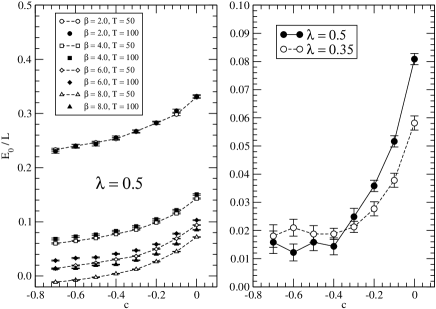
FIG. 2.: Ground state energy per site $E_{0}/L$. The left graph shows the intermediate results at variable $\varepsilon$ and $\beta$. The right graph shows the extrapolation to $\epsilon\to 0$ followed by $\beta\to\infty$.

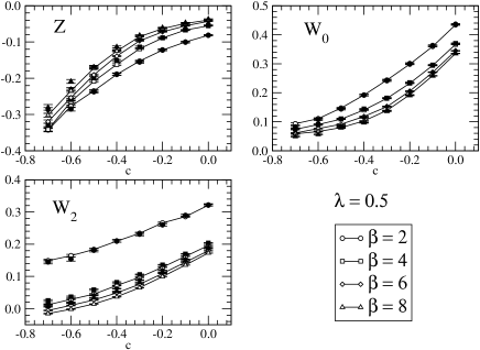
FIG. 3.: Intermediate results for $Z$ and $W_{0,2,4}$. Empty (full) symbols are obtained on the $22\times 50$ ($22\times 100$) lattice.

The systematic error due to $\varepsilon$ increases with $\beta$ at fixed $T$ simply because the corresponding $\varepsilon$ is bigger. The limit $\varepsilon\to 0$ is absolutely necessary and, in particular, restores positivity of $E_{0}$ at large $\beta$. As $c$ is decreased, the extrapolated $E_{0}$ reaches a positive plateaux. This residual value is slightly higher at $\lambda=0.35$, due to the larger finite volume effects. The beginning of the flat region is at $c(0.5)\simeq-0.4$ and $c(0.35)\simeq-0.3$, in agreement with Eq. (15). In Fig. (3) we show the intermediate data for $Z$ and $W_{0,2}$. It is interesting to note that $W_{0}$ is quite independent on $\varepsilon$ at the explored values and is thus the most safe quantity to be analyzed. Fig. (4) collects the extrapolated data.

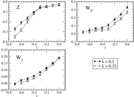
FIG. 4.: Extrapolated results for $Z$, $W_{0,2,4}$ obtained from the data shown in Fig. (3).

The central charge $Z$ is definitely negative with a sharp variation around $c\simeq-0.3$. If SUSY is to be recovered in the $L\to\infty$ limit, we expect BPS states to be present together with eventual $Q=Z=0$ states. The sign of $Z$ is easily checked: in the ${\rm WZ}_{1}$ model we have $Q_{1}^{2}=P^{0}+Z$ and $P^{0}=Q_{1}^{2}+Q_{2}^{2}$ is a positive operator. Hence, states in the lowest $Q_{1}^{2}$ eigenspace prefer $Z<0$ and states with $Q_{1}=0$ have rigorously $Z\leq 0$. The Ward identities are all non zero although $W_{0}$ and $W_{2}$ approach smaller values as $c$ decreases. Again $W_{0}$ flattens below $c\simeq-0.3$. We conclude that SUSY is broken (at $L=22$) for all $c$ in agreement with the GFMC analysis of [4] and the analytical arguments [7]. The SUSY restoration observed in [6] must be explained in terms of the moderate statistical errors. Indeed, as we have shown, the absolute values of $E_{0}$ are quite small and arise from large cancellations between contributions from $H_{B}$ and $H_{F}$. The search for SUSY restoration requires a suitable finite size scaling analysis of data at rather larger $L$. The critical point is to be searched around $c=-0.4(-0.3)$ for the considered $\lambda=0.5(0.35)$. Indeed, the presented results suggest some kind of transition there.

In the final part of this Report we want to show how a consistent additional information is provided by the fluctuations of the central charge $Z$. In the continuum, $Z$ is a global quantity depending on the boundary conditions. On the lattice, its geometrical meaning is not clear due to the quantum roughness of the configurations. An histogram analysis of $Z$ reveals that definite non-Gaussian fluctuations are present. The density of the normalized variable $\zeta=(Z-\langle Z\rangle)/(\langle Z^{2}\rangle-\langle Z\rangle^{2})^{1/2}$ turns out to be consistent with the generalized Gumbel one [11]

$$P(\zeta)={\cal N}\exp[\alpha\ (\mu\zeta+\nu-e^{\mu\zeta+\nu})],$$ (16)

where ${\cal N}$, $\mu$ and $\nu$ are functions of $\alpha$ fixed by normalization, zero mean and unit variance. Fig. (5) shows the best fit coefficient $\alpha(c)$ and two sample spectra.

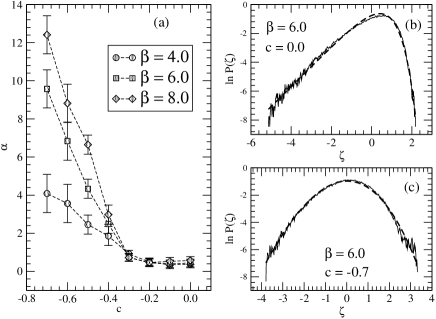
FIG. 5.: Analysis of $Z$ ($\lambda=0.35$). The graph (a) shows the coefficient $\alpha$ (defined in the text) as a function of $c$. The graphs (b,c) show two sample fluctuation spectra together with the best fit with Eq. (16).

In Fig. (5, a) a change of behaviour occurs around $c^{*}\simeq-0.3$. When $c\geq c^{*}$, $\alpha(c)$ is small and weakly dependent on both $c$ and $\beta$. Below $c^{*}$, $\alpha(c)$ increases rapidly as $c$ is decreased and the slope is larger as $\beta$ increases. The values of the fitted $\mu$, $\nu$ for large $\alpha$ are such that $\sqrt{\alpha}\mu\to 1$ and $\sqrt{\alpha}\nu\to 0$. For $\alpha\to\infty$, the limiting form of Eq. (16) converge to a normal Gaussian. Indeed the spectrum asymmetry decreases as $c$ crosses $c^{*}$. For instance, Fig. (5, c) is almost consistent with a simpler Gaussian fit. Similar features are discussed in [8] where the particular value $\alpha=\pi/2$ is observed and related to the joint effect of finite-size, strong correlation and self-similarity. In the ${\rm WZ}_{1}$ model, the quantum symmetry breaking is not explained in terms of self-similar structures and $\alpha$ is just a measure of the deviation from Gaussian statistics. It is tempting to interpret Fig. (5) as another signal for a finite size critical $c^{*}(L)$ with SUSY restoration in infinite volume at $c=c^{*}(\infty)$. At a qualitative level, in the symmetric phase soliton states appear with a definite $Z$ and the MC measures fluctuate with a normal distribution. In the broken phase $Z$ is expected to vanish, but an inspection of the MC histories shows that rare configurations appear with unphysical kinks responsible for the tail of $P(\zeta)$ at negative $\zeta<0$. Further analysis is needed to determine the precise functional form of $Z$, particularly at large $|\zeta|$, and to clarify its relation with the $L=\infty$ SUSY transition. However, Fig. (5, a) demonstrates clearly that the study of $P(\zeta)$ is in principle rich of information. It is a pleasure to thank M. Campostrini and A. Feo for discussions about the ${\rm WZ}_{1}$ model and E. Alfinito for bringing the role of extremal statistics to our attention. Financial support from INFN, IS-RM42 is acknowledged.

REFERENCES

- [1] A. Feo, Supersymmetry on the lattice, Plenary talk at 20th Int. Symposium on Lattice Field Theory (LATTICE 2002), Boston, Massachusetts, hep-lat/0210015. For WZ models in 1+1 see also [6] below and M. Beccaria, E. D’Ambrosio, G. Curci, Phys. Rev. D 58, 065009 (1998); S. Catterall, E. Gregory, Phys. Lett. B 487, 349 (2000); S. Catterall, S. Karamov, Phys. Rev. D 65, 094501 (2002); K. Fujikawa, ibid. 66, 074510 (2002).
- [2] L. Alvarez-Gaume, D. Z. Freedman, M. T. Grisaru, Spontaneous breakdown of supersymmetry in two-dimensions, Brandeis U. preprint HUTMP 81/B111, unpublished.
- [3] Recent papers exploiting GFMC methods in lattice models with no supersymmetry are: M. Beccaria and A. Moro, Phys. Rev. D 64, 077502 (2001); M. Beccaria, ibid. 62, 034510 (2000); 61, 114503 (2000); Eur. Phys. J. C 13,357 (2000); C.J. Hamer, M. Samaras, R.J. Bursill, Phys. Rev. D 62, 074506 (2000); 62, 054511 (2000);
- [4] M. Beccaria, M. Campostrini, A. Feo, Nucl. Phys. B (Proc. Suppl.) 106, 944 (2002); M. Beccaria, M. Campostrini, A. Feo, 20th Int. Symposium on Lattice Field Theory (LATTICE 2002), Boston, Massachusetts, hep-lat/0209010 to appear on Nucl. Phys. B (Proc. Suppl.); M. Beccaria, M. Campostrini and A. Feo, in preparation.
- [5] The first reference to WLPI is J. E. Hirsch, R. L. Sugar, D. J. Scalapino, R. Blanckenbecler, Phys. Rev. B 26, 5033 (1982).
- [6] J. Ranft, A. Schiller, Phys. Lett. B 138, 166 (1984); J. Phys. G 12, 935 (1986).
- [7] E. Witten, Nucl. Phys. B 202, 253 (1982).
- [8] S. T. Bramwell et al., Phys. Rev. E 63, 041106 (2001); S. T. Bramwell et al., Phys. Rev. Lett. 84, 3744 (2000); S. T. Bramwell, P. C. W. Holdsworth and J.-F. Pinton, Nature 396, 552 (1998);
- [9] E. Witten and D. Olive, Phys. Lett. 78 B, 97 (1978).
- [10] S. Elitzur, E. Rabinovici, A. Schwimmer, Phys. Lett. B 119, 165 (1982); S. Elitzur and A. Schwimmer, Nucl. Phys. B 226, 109 (1983).
- [11] E. J. Gumbel, Statistics of Extremes, Columbia University Press, New York, (1958). Phys. Rev. D Server