An Application of Feynman-Kleinert Approximants to the Massive Schwinger Model on a Lattice

Abstract

A trial application of the method of Feynman-Kleinert approximants is made to perturbation series arising in connection with the lattice Schwinger model. In extrapolating the lattice strong-coupling series to the weak-coupling continuum limit, the approximants do not converge well. In interpolating between the continuum perturbation series at large fermion mass and small fermion mass, however, the approximants do give good results. In the course of the calculations, we picked up and rectified an error in an earlier derivation of the continuum series coefficients.

I INTRODUCTION

The analytic continuation of a function, whose perturbation series expansion about a given point is known, is an important and long-standing problem. Some standard methods are the use of Padé approximants, or integrated differential approximants, as reviewed for instance by Guttmann[1]. In some circumstances, these techniques can work extremely well; but in others they fail. A well known difficult case is that of a function whose series expansion about the origin in a variable $x$, say, is known up to a given order, and we want to extrapolate to $x\rightarrow\infty$. If there is a cut or an essential singularity at infinity, the standard methods do not work well. This is a common situation in lattice gauge theory, for instance.

In recent years, a new method has been developed, involving “Feynman-Kleinert approximants”[2]. This is a variational technique, arising originally from a Gaussian approximation to the path integral[3]. It has been used with great success on a number of problems, such as extrapolation of the weak-coupling series for the anharmonic oscillator[4], where the asymptotic strong-coupling behaviour was obtained with extraordinary accuracy, up to 20 significant digits. For a discussion and further references, see the recent paper by Kleinert[5].

Here we attempt to apply the new method to a lattice gauge theory, namely the Schwinger model in (1+1) dimensions. In the series approach to lattice gauge theory, one generates strong-coupling series expansions for the physical quantities of interest, and then tries to extrapolate to the continuum, weak-coupling limit. It would be an important breakthrough if a better technique could be found for performing this extrapolation. In the report we set out to test whether Feynman-Kleinert approximants can fulfill this need. Unfortunately, we find that the technique is not very successful in this context.

Another common problem is that of interpolation of a function, where a number of series coefficients are known of both the weak-coupling and the strong-coupling expansions. An example of this arises for the low-lying energy eigenvalues in the continuum Schwinger model, as functions of $m/g$, where $m$ is the fermion mass and $g$ is the electric coupling. We show that Feynman-Kleinert approximants can provide an effective interpolation between these two limits.

II THEORY

For reference, let us briefly recapitulate the algorithm set out by Kleinert[2] using his notation. Consider a quantity $E$ whose perturbation series expansion in some parameter $\alpha$ is known to order $N$:

$$E_{N}=\sum_{n=0}^{N}a_{n}\alpha^{n}.$$ (1)

Write

$$E_{N}^{\omega}=\omega^{p}\sum_{n=0}^{N}a_{n}\left(\frac{\alpha}{\omega^{q}}\right)^{n},$$ (2)

where $\omega$ is an auxiliary parameter whose value will eventually be set equal to 1, and $p,q$ are indices which will be chosen later to suit the problem at hand. Now set $\omega\equiv\sqrt{\Omega^{2}+\omega^{2}-\Omega^{2}}$, and re-expand $E_{N}^{\omega}$ in powers of $\lambda=1-\omega^{2}/\Omega^{2}$, treating $\lambda$ as a quantity of order $\alpha$, and truncating the re-expanded series at order $N$. The result is a function

$$W_{N}(\alpha,\Omega)=\Omega^{p}\sum_{n=0}^{N}a_{n}f_{n}(\Omega)\left(\frac{\alpha}{\Omega^{q}}\right)^{n},$$ (3)

where

$$f_{n}(\Omega)=\sum_{j=0}^{N-n}\left(\begin{array}[]{c}(p-qn)/2\\ j\end{array}\right)(-1)^{j}\left(1-\frac{\omega^{2}}{\Omega^{2}}\right)^{j}.$$ (4)

Forming the first and second derivatives of $W_{N}(\alpha,\Omega)$ with respect to $\Omega$ (and setting $\omega=1$), we find the positions of the turning points. The smallest among these is denoted $\Omega_{N}$. The resulting $W_{N}(\alpha)\equiv W_{N}(\alpha,\Omega_{N})$ gives the desired approximation to the function $E$ at finite $\alpha$, an extrapolation of the function $E_{N}$ to finite $\alpha$.

Now consider the limit $\alpha\rightarrow\infty$. At large $\alpha$, $\Omega_{N}$ will scale with $\alpha$ like

$$\Omega_{N}\sim\alpha^{1/q}c,$$ (5)

so that

$$W_{N}(\alpha,\Omega_{N})\sim\alpha^{p/q}.$$ (6)

The full ‘strong-coupling’ (large $\alpha$) expression can now be obtained by writing

$$W_{N}(\alpha,\Omega)=\Omega^{p}w_{N}(\hat{\alpha},\omega^{2}/\Omega^{2}),$$ (7)

with $\hat{\alpha}=\alpha/\Omega^{q}$, and expanding $w_{N}$ in powers of $\omega^{2}/\Omega^{2}$, which for $\alpha\rightarrow\infty$ behaves like $(1/c^{2})(\alpha/\omega^{q})^{-2/q}$. The result is

$$W_{n}(\alpha)=\alpha^{p/q}\left[b_{0}(c)+b_{1}(c)\left(\frac{\alpha}{\omega^{q}}\right)^{-2/q}+b_{2}(c)\left(\frac{\alpha}{\omega^{q}}\right)^{-4/q}+\dots\right]$$ (8)

with

$$b_{n}(c) = \frac{1}{n!}w_{N}^{(n)}(\hat{\alpha},0)\left.\hat{\alpha}^{(2n-p)/q}\right|_{\hat{\alpha}=1/c^{q}}$$ (9)

$$= \sum_{l=0}^{N}a_{l}\sum_{j=n}^{N-l}\left(\begin{array}[]{c}(p-lq)/2\\ j\end{array}\right)\left(\begin{array}[]{c}j\\ n\end{array}\right)(-1)^{j-n}c^{p-lq-2n}.$$ (14)

The indices $p$ and $q$ in the expansion (2) are now chosen so as to give the correct asymptotic behaviour (i.e. the correct powers of $\alpha$) in the strong-coupling expansion (8), which we assume is known a priori. The leading coefficient $c$ in (5) is found by searching for the extrema of the leading coefficient $b_{0}(c)$ as a function of $c$ and choosing the smallest of them.

Finally, we have to account for the fact that $\Omega_{N}$ will have corrections to the leading behaviour $\alpha^{1/q}c$. We can allow for this by replacing $c$ by

$$c(\alpha)=c_{0}+c_{1}\left(\frac{\alpha}{\omega^{q}}\right)^{-2/q}+c_{2}\left(\frac{\alpha}{\omega^{q}}\right)^{-4/q}+\dots$$ (15)

requiring a re-expansion of the coefficients $b_{n}(c)$ in (14). The expansion coefficients $c_{n}$ are determined by looking for the turning points of $b_{2n}(c)$, successively.

The equations

$$\frac{db_{2n}(c)}{dc_{n}}=0,$$ (16)

together with knowledge of the coefficients $\{a_{n},n=0,\dots,N\}$, can in principle be used to determine a set of parameters $\{c_{n},n=0,\dots,N\}$, and hence estimate the leading strong-coupling coefficients $b_{n}(c)$. This provides estimates of the asymptotic behaviour of the function $E$. In the case of the strong-coupling anharmonic oscillator, it has been shown[4] that the resulting estimates converge exponentially fast, and have been used to estimate the energy eigenvalue in the strong-coupling limit accurate to 20 decimal places!

Alternatively, any knowledge of the strong-coupling coefficients $b_{0},b_{1},\dots$ can be fed back into the set of equations (14) and (16) to obtain estimates of further weak-coupling coefficients $a_{N+1},a_{N+2},\dots$, and thus carry the extrapolation $W_{N}(\alpha)$ to higher orders. This is the basis of the interpolation algorithm between weak and strong-coupling for the function $E$.

III RESULTS

A Extrapolation to the Continuum Limit

We have applied the Feynman-Kleinert approximation method to the lattice Schwinger model, as formulated by Banks et al. [6]. The rescaled lattice Hamiltonian is

$$W=\frac{2}{ag^{2}}H=W_{0}+xV,$$ (17)

where

$$W_{0}=\sum_{n}L^{2}(n)+\mu\sum_{n}(-1)^{n}\phi^{\dagger}(n)\phi(n),$$ (18)

$$V=-i\sum_{n}\left[\phi^{\dagger}(n)e^{i\theta(n)}\phi(n+1)-\mbox{h.c.}\right],$$ (19)

and

$$\mu=\frac{2m}{g^{2}a},\hskip 28.45274ptx=\frac{1}{g^{2}a^{2}}.$$ (20)

Here $m$ is the electron mass, $g$ is the electric coupling constant, and $a$ is the lattice spacing. The field $\phi(n)$ is the lattice fermion field defined on sites $n$,

$$\{\phi(n),\phi^{\dagger}(m)\}=\delta_{nm},$$ (21)

while $L(n)$ is the electric field on link $n$, which takes only integer eigenvalues.

Expansions of the energy eigenvalues of the operator $W$ have been calculated to high orders in the perturbation parameter $x$, using efficient linked cluster methods[7]. Our object now is to see whether these series can be accurately extrapolated to the continuum limit, which corresponds to $a\rightarrow 0$ or $x\rightarrow\infty$, using the Feynman-Kleinert approach.

1 Ground State Energy

For the ground state energy per site $\omega_{0}/M$, where $M$ is the number of states, the series expansion is of the form

$$\omega_{0}/M=\sum_{n}a_{n}\left(x^{2}\right)^{n},$$ (22)

where $a_{0}=0$; and the asymptotic behaviour as $x\rightarrow\infty$ is known[6]

$$\omega_{0}/M\sim-\frac{2x}{\pi}.$$ (23)

The coefficients $a_{n}$ have been calculated up to order $n=15$ [7]. In this case, we can apply the formalism of section II, taking $E=\omega_{0}/M$, $\alpha=x^{2}$, $p=2$, $q=4$, which implies the asymptotic behaviour as $x\rightarrow\infty$

$$\omega_{0}/M\sim b_{0}x+b_{1}+O(x^{-1}).$$ (24)

Fig. 1 shows the resulting approximants to the ground-state energy at $m/g=0$ compared with numerical results obtained by other methods, and the known continuum limit, Eq. (23). It can be seen that the approximants do seem to converge to the correct limit, but only rather slowly.

2 Energy Gap

The energy gap to the lowest-lying positronium state has an expansion

$$\omega_{1}-\omega_{0}=\sum_{n}a_{n}\left(x^{2}\right)^{n}$$ (25)

and the expected asymptotic behaviour as $x\rightarrow\infty$ is

$$\omega_{1}-\omega_{0}\sim b_{0}x^{1/2}.$$ (26)

The coefficients $a_{n}$ for this series have been calculated up to order $n=14$ [7]. Here, we take $\alpha=x^{2}$, $p=2$, $q=8$, assuming the asymptotic behaviour as $x\rightarrow\infty$

$$\omega_{1}-\omega_{0}\sim b_{0}x^{1/2}+b_{1}+O(x^{-1/2})$$ (27)

which accords with previous studies[7, 8]. In this case, however, the Feynman-Kleinert approximants do not converge at all at large $x$. Fig. 2 shows the dependence of the estimated value of $b_{0}$ as a function of the parameter $c_{0}$, for the case $m/g=0$, at various orders $N$. It can be seen that as $c_{0}$ increases, the estimate of $b_{0}$ comes in from infinity, oscillates around the correct value (marked by a solid line ), and then slowly drifts away again. Unfortunately, the oscillations increase with order $N$, and the values at the lowest turning point correspondingly diverge away from the correct value as $N$ increases. The same is true of the values at the lowest point of inflection. It seems that the Feynman-Kleinert approximant method fails in this case.

B Interpolation of Continuum Series

Another problem connected with series expansions for the Schwinger model arises in connection with the continuum field theory, rather than the lattice model. A few coefficients are known of the series expansions for the lowest-lying excited states of the model, the “vector” and “scalar” positronium states, in both the strong-coupling and weak-coupling regimes. At strong coupling, $m/g\rightarrow 0$, the first three coefficients have been computed by Adam[9], using the bosonic form of the theory:

$$\frac{E}{g}=\left(\frac{M-2m}{g}\right)=\sum_{n}a_{n}\left(m/g\right)^{n}.$$ (28)

At weak coupling, $m/g\rightarrow\infty$, the first three coefficients have been calculated by Sriganesh et al. [11], following a treatment of Coleman [10]:

$$\frac{E}{g}\sim\left(\frac{g}{m}\right)^{1/3}\sum_{n}b_{n}\left[\left(\frac{g}{m}\right)^{2/3}\right]^{n}.$$ (29)

The problem now is, how can one compute a sensible interpolation between these two series to obtain accurate estimates of the energy eigenvalues at finite $m/g$? One possibility is to use “2-point” Padé approximants: but they involve only integer powers of the variable, $(m/g)$ in this case. By fitting an appropriate power of the function $E/g$ one can mimic the leading behaviour as $m/g\rightarrow\infty$, but cannot reproduce the sub-leading powers. Furthermore, experience shows that 2-point Padé approximants are prone to exhibit spurious ‘wiggles’ at intermediate couplings between the two limits. Here we set out to apply Feynman-Kleinert approximants to the problem.

Setting $\alpha=m/g$, $p=1$, $q=3$, we have computed Feynman-Kleinert approximants for the energy eigenvalues using known values for the coefficients $\{a_{n},b_{n},n=0,N-1\}$ for $N=1,2,3$. Now knowing $2N$ coefficients in total allows us to estimate the next $N$ coefficients for either the $a_{n}$ or $b_{n}$ series. Table I shows the ‘predicted’ values versus the known values for $N=1$. For the vector state with $N=1$, the predicted values are in quite good agreement with the known values, to within a few percent. At $N=2$ (see Table II), however, a large discrepancy becomes evident between the predicted and ‘known’ values for the coefficient $b_{2}$ - even the sign is different. This prompted us to re-examine the calculation of the weak-coupling coefficients $b_{n}$ by Sriganesh et al.[11]; and indeed we discovered some errors in those calculations. A corrected version of the calculations is given in the Appendix; the corrected series coefficients are also shown in Table II.

For the scalar state, the ‘predicted’ series coefficients disagree with the known ones even at $N=1$ - but this is easily understood, in that the simplest interpolation between the zeroth order series at either end would have no ‘hump’ in the middle such as is shown in Fig. 4. The predicted values at $N=2$ agree qualitatively with the (corrected) known values.

The Feynman-Kleinert approximants were found to give smooth and apparently accurate interpolations of the energy eigenvalues at finite $m/g$, up to order $N=2$. At order $N=3$, no solution was found to the system of simultaneous equations - we have not explored in detail why this occurred. Figures 3 and 4 show the results for the vector and scalar state interpolations. For the vector state energies, our interpolation is compared to data obtained from the density matrix renormalization group (DMRG) method [8], the “fast moving frame” estimates of Kröger and Scheu [12], and the “renormal-ordered” mass perturbation series results of Adam [14]. The scalar state interpolations are compared to the finite lattice calculations of Sriganesh et al. [11], and again results of Kröger and Scheu, and Adam. Both plots show excellent agreement between the interpolation and the numerical data, within errors. We also plot the second order strong and weak coupling series used to generate the interpolation on the same plots, which diverge away for large and small masses respectively. The “renormal-ordered” expansion [14] about $m/g=0$, extends the region of validity of the perturbation theory, and agrees fairly well with our interpolation for small masses.

The interpolation performs particularly well for the scalar state, where for small $m/g$, the original strong coupling series disagrees significantly with the numerical data. The interpolation on the other hand agrees extremely well with existing results, despite the large gap that must be bridged between the two series. Tables III and IV list numerical values for specific values of $m/g$ for the interpolation compared to previous works. We estimate the error on our interpolations based on the difference between our quoted $N=2$ calculation and the corresponding $N=1$ calculation. Error estimates have probably been overestimated somewhat using this method, as can be seen from the good agreement with the numerical data in Figure 4. We have not however found a better way of estimating these errors.

IV CONCLUSIONS

The Feynman-Kleinert approximants have earned a mixed scorecard in the applications we have discussed. For the extrapolation of lattice strong-coupling series to the weak-coupling continuum limit, the approximants have basically failed. They converged for the ground-state eigenvalue, but only slowly; and for the first excited state eigenvalue, they did not converge at all. This is probably due to the presence of exponentially decaying terms corresponding to essential singularities in the weak-coupling limit, which are not accounted for in the Feynman-Kleinert approach. The upshot is, unfortunately, that this approach does not seem to have any advantage over previous techniques[7], which used Padé or integral approximants to extrapolate to intermediate couplings, and then ‘matched’ the results onto a weak coupling form to reach the continuum limit.

For the continuum field theory, however, the Feynman-Kleinert approximants have proved useful in providing a sensible and apparently accurate interpolation between the known weak coupling and strong coupling series. The fact that we were able to pick up a mistake in the series coefficients by this approach adds confidence in the technique. No doubt many applications of a similar nature are possible.

A WEAK COUPLING EXPANSION OF THE MASSIVE SCHWINGER MODEL

Our starting point is the Hamiltonian as derived by Coleman in the two-particle subspace (see Eq. (4.18) of Ref. [10]). We set the background field $\theta=0$. Expanding this Hamiltonian for large mass $m$, and keeping terms to order $O(m^{-3})$ we obtain a Schrödinger equation

$$(H_{0}+H_{1})\psi(x)=E\psi(x),$$ (A1)

where

$$H_{0} = -\frac{1}{m}\frac{\partial^{2}}{\partial x^{2}}+\frac{g^{2}}{2}|x|$$ (A2)

$$H_{1} = -\frac{g^{2}}{m\pi}-\frac{1}{4m^{3}}\frac{\partial^{4}}{\partial x^{4}}+\frac{g^{2}}{4m^{2}}\delta(x)-\frac{g^{2}}{2\pi m^{3}}\frac{\partial^{2}}{\partial x^{2}}.$$ (A3)

Rescale to dimensionless variables as follows:

$$x=\left(\frac{2}{mg^{2}}\right)^{1/3}z\hskip 28.45274ptE=\left(\frac{g^{4}}{4m}\right)^{1/3}\epsilon.$$ (A4)

Then (A1) becomes

$$(H^{\prime}_{0}+H^{\prime}_{1})\psi(z)=\epsilon\psi(z),$$ (A5)

where

$$H^{\prime}_{0} = -\frac{\partial^{2}}{\partial z^{2}}+|z|$$ (A6)

$$H^{\prime}_{1} = -\frac{1}{\pi}\left(\frac{2g}{m}\right)^{2/3}-\left(\frac{g}{4m}\right)^{4/3}[\frac{\partial^{4}}{\partial z^{4}}-2\delta(z)].$$ (A7)

The last term in (A2) has now been dropped as it is now clear it is of order $\sim(g/m)^{2}$. The solution of the leading-order Schrödinger equation

$$\left(\frac{d^{2}}{dz^{2}}-|z|\right)\psi(z)=-\epsilon\psi(z),$$ (A8)

was discussed by Hamer[13]. The solution of (A8) is a symmetric or antisymmetric Airy function which obeys the condition

$$\mbox{Ai}^{\prime}(-\epsilon_{n})=0$$ (symmetric) (A9)

$$\mbox{Ai}(-\epsilon_{n})=0 \hskip 28.45274pt\mbox{(antisymmetric)}.$$ (A10)

The lowest symmetric (antisymmetric) wavefunction gives the energy for the vector (scalar) state.

The higher order terms contained in $H^{\prime}_{1}$ may be taken into account by calculating the correction term $\Delta\epsilon=\langle\psi|H^{\prime}_{1}|\psi\rangle$ using numerical integration (the results are shown in Table V). Rescaling back to our original variables gives us

$$\frac{E_{1}}{g}=0.6418\left(\frac{g}{m}\right)^{1/3}-\frac{1}{\pi}\left(\frac{g}{m}\right)+0.1547\left(\frac{g}{m}\right)^{5/3},$$ (A11)

for the vector state binding energy, and

$$\frac{E_{2}}{g}=1.473\left(\frac{g}{m}\right)^{1/3}-\frac{1}{\pi}\left(\frac{g}{m}\right)-0.1093\left(\frac{g}{m}\right)^{5/3}.$$ (A12)

for the scalar state binding energy.

TABLE I.: Comparison of known coefficients in weak [11] and strong [9] coupling series, versus the Feynman-Kleinert estimates (labeled as “Predicted”). Feynman-Kleinert estimates are obtained by starting with zeroth order coefficients $a_{0}$ and $b_{0}$ (i.e. $N=1$), for each of the vector and scalar particle states.

Coefficient	Vector State		Scalar State
	Predicted	Known	Predicted	Known
$a_{1}$	-0.2046	-0.2189	-0.2709	1.562
$b_{1}$	-0.2917	-0.3183	-0.8813	-0.3183

TABLE II.: As for Table I, but with $N=2$. The “known” coefficients for $b_{2}$ contain both the result obtained in Ref. [11] (in square brackets), and our recalculation (unbracketed).

Coefficient	Vector State		Scalar State
	Predicted	Known	Predicted	Known
$a_{2}$	0.2298	0.1907	-10.13	-13.51
$a_{3}$	-0.3148		49.01
$b_{2}$	0.2159	0.1547 [-0.2521]	-0.1854	-0.1093 [0.1085]
$b_{3}$	-0.1669		0.2794

TABLE III.: Comparison of interpolation results for the vector state with numerical results obtained by Byrnes et al. [8], Kröger and Scheu [12], and Adam [14].

$m/g$	This work	Byrnes	Kröger and	Adam [14]
		et al. [8]	Scheu [12]
0.125	0.540(2)	0.53950(7)	0.528	0.539
0.25	0.520(3)	0.51918(5)	0.511	0.516
0.5	0.490(4)	0.48747(2)	0.489	0.474
1	0.448(4)	0.4444(1)	0.455	0.43
2	0.396(4)	0.398(1)	0.394	0.49
4	0.341(3)	0.340(1)	0.339	0.76
8	0.287(2)	0.287(8)	0.285	1.40
16	0.237(2)	0.238(5)	0.235	2.75

TABLE IV.: Comparison of interpolation results for the scalar state with numerical results obtained by Sriganesh et al. [11], Kröger and Scheu [12], and Adam [14].

$m/g$	This work	Sriganesh	Kröger and	Adam [14]
		et al. [11]	Scheu [12]
0.125	1.23(13)	1.22(2)	1.314	1.220
0.25	1.24(17)	1.24(3)	1.279	1.230
0.5	1.21(19)	1.20(3)	1.227	1.165
1	1.12(17)	1.12(3)	1.128	0.99
2	0.99(13)	1.00(2)	0.991	0.88
4	0.84(8)	0.85(2)	0.837	1.07
8	0.69(5)	0.68(1)	0.690	1.78
16	0.56(3)	0.56(1)	0.559	3.41

TABLE V.: Results of numerical integration over symmetric and antisymmetric states for two operators.

Integral	Symmetric	Antisymmetric
$\langle\frac{\partial^{4}}{\partial z^{4}}\rangle_{0}$	-0.577655	1.093349
$\langle\delta(z)\rangle_{0}$	0.490777	0.0

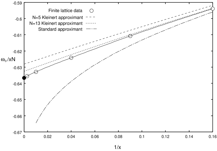
FIG. 1.: Ground state energy per site of the lattice Schwinger model at $m/g=0$, as obtained by the Kleinert approximants with $N=5$ and $N=13$. Open circles denote finite lattice calculations, the closed circle shows the position of the exact result in the continuum limit, $\omega_{0}/xN=-2/\pi$. We also show an extrapolation using a standard Padé approximant for comparison.

FIG. 2.: Dependence of the value $b_{0}$ as a function of $c_{0}$ for the case $m/g=0$, at four orders in $N$. The exact result is shown as a solid line at $b_{0}=2/\sqrt{\pi}\approx 1.128$.

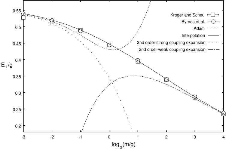
FIG. 3.: A comparison of the Feynman-Kleinert interpolation for the vector state with numerical DMRG data of Byrnes et al. [8], “fast moving frame” estimates of Kröger and Scheu [12], and the “renormal-ordered” mass perturbation theory results of Adam [14]. The 2nd order ($N=2$) weak and strong coupling series, which are used to generate the interpolation, are also shown for comparison.

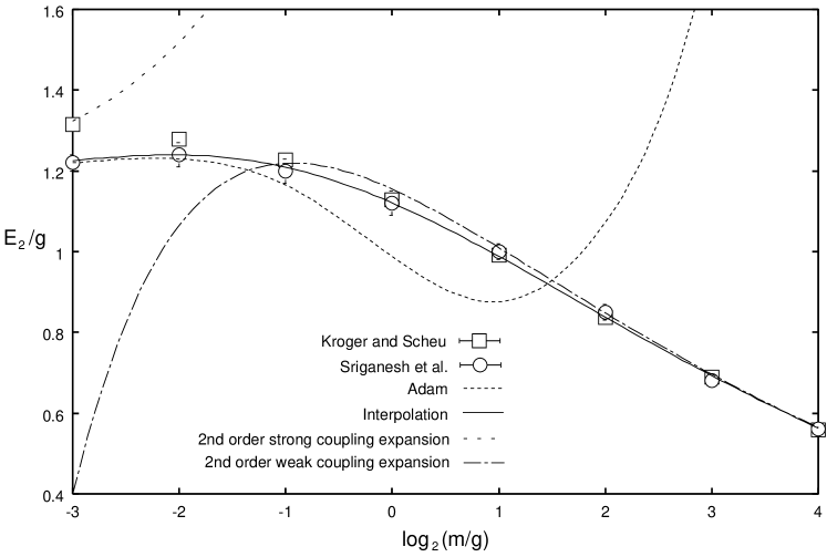
FIG. 4.: A comparison of the Feynman-Kleinert interpolation for the scalar state to finite lattice estimates of Sriganesh et al. [11], “fast moving frame” estimates of Kröger and Scheu [12], and the “renormal-ordered” mass perturbation theory results of Adam [14]. The 2nd order ($N=2$) weak and strong coupling series, which are used to generate the interpolation, are also shown for comparison.

REFERENCES

- [1] A.J. Guttmann, in Phase Transitions and Critical Phenomena, ed. C. Domb and J.L. Lebowitz (Academic, New York, 1989), Vol. 13.
- [2] H. Kleinert, Phys. Letts. A207, 133 (1995).
- [3] R.P. Feynman and H. Kleinert, Phys. Rev. A34, 5080 (1986).
- [4] W. Janke and H. Kleinert, Phys. Rev. Letts. 75, 2787 (1995).
- [5] H. Kleinert, Phys. Rev. D57, 2264 (1998).
- [6] T. Banks, L. Susskind, and J. Kogut, Phys. Rev. D 13, 1043 (1976).
- [7] C.J. Hamer, Zheng W-H. and J. Oimaa, Phys. Rev. D56, 55 (1997).
- [8] T.M.R. Byrnes, P. Sriganesh, R.J. Bursill, and C.J. Hamer, Phys. Rev D 66, 013002 (2002).
- [9] C. Adam, Phys. Lett. B 382, 383 (1996); Ann. Phys. (N.Y.) 259, 1 (1997).
- [10] S. Coleman, Ann. Phys. (N.Y.) 101, 239 (1976).
- [11] P. Sriganesh, C. J. Hamer, and R. J. Bursill, Phys. Rev. D 62, 034508 (2000).
- [12] H. Kröger and N. Scheu, Phys. Lett. B 429, 58 (1998).
- [13] C.J. Hamer, Nucl. Phys. B 121, 159 (1977).
- [14] C. Adam, hep-th/0212171.