Chiral Limit of Strongly Coupled Lattice Gauge Theories

Abstract

We construct a new and efficient cluster algorithm for updating strongly coupled $U(N)$ lattice gauge theories with staggered fermions in the chiral limit. The algorithm uses the constrained monomer-dimer representation of the theory and should also be of interest to researchers working on other models with similar constraints. Using the new algorithm we address questions related to the chiral limit of strongly coupled $U(N)$ gauge theories beyond the mean field approximation. We show that the infinite volume chiral condensate is non-zero in three and four dimensions. However, on a square lattice of size $L$ we find $\sum_{x}\ \langle\bar{\psi}\psi(x)\ \bar{\psi}\psi(0)\rangle\sim L^{2-\eta}$ for large $L$ where $\eta=0.420(3)/N+0.078(4)/N^{2}$. These results differ from an earlier conclusion obtained using a different algorithm. Here we argue that the earlier calculations were misleading due to uncontrolled autocorrelation times encountered by the previous algorithm.

I INTRODUCTION

One of the challenges in the study of strong interactions is to compute physical quantities with in the framework of QCD with controlled errors. Although lattice QCD can in principle accomplish this task, most known algorithms encounter problems related to critical slowing down as the quark masses become small Ber02 . It is impossible to compute quantities reliably for realistic “up” and “down” quark masses with current algorithms. At present, one usually computes quantities at an unphysically large quark mass and uses chiral extrapolations to obtain the final answer Ber102 . For sufficiently light quarks this is a reliable technique. However, for the quark masses that are currently used, such extrapolations are questionable. Furthermore, most calculations with light quarks are obtained in the quenched approximation where the internal dynamics of fermions are ignored. There also exist some interesting quantities which cannot be computed when the quarks are heavy. For example, in the real world the rho meson can decay into two pions. Unfortunately, for most values of the quark masses that are currently used, this decay is forbidden. If lattice simulations were possible with sufficiently light quarks, the resonant nature of the rho meson can be studied with lattice techniques Lus91 .

There are two main problems in constructing efficient algorithms for lattice QCD. The first is that the fundamental variables, namely the quark and gluon fields, are unphysical since they are gauge dependent. Secondly, the quarks are fermions and due to the Pauli principle introduce sign problems which are typically very difficult to solve. Fortunately, with a good lattice fermion formulation and at zero baryon chemical potential, the second problem can be avoided. The quarks can be integrated out and their effects can be encoded in terms of a determinant which is a positive non-local function of the gauge fields. However, one is still left with the problem of updating the unphysical gauge fields. Previous experience suggests that in order to find an efficient algorithm it is often useful to understand and isolate the physical modes of the theory. Unfortunately, for gauge theories, especially with the non-local fermion determinant this problem looks formidable.

Interestingly, there is a limit of lattice QCD with staggered fermions where most of the above mentioned complications can be eliminated. This is the so called strong coupling limit Dro83 . Although this limit has the worst lattice artifacts and could describe the wrong phase, the resulting theory is still an interesting toy model for QCD. It contains the physics of confinement and chiral symmetry breaking. In the chiral limit one finds massless Goldstone bosons in addition to other massive mesonic and baryonic excitations. The strong coupling theory can be solved analytically only in the large $N$ Kaw81 and large $d$ Klu83 limits. One needs a numerical approach to study it without these approximations.

The luxury of the strong coupling limit is that it is possible to integrate out the gauge fields analytically and write the problem entirely in terms of gauge invariant objects. It was pointed out in Wol84 that with $U(N)$ gauge fields the strong coupling model with staggered fermions is equivalent to a system of monomers and dimers with positive Boltzmann weights. Later a monomer-dimer-polymer representation was discovered for $SU(3)$ gauge fields Kar89 . Is it possible to use these simplified representations that arise at strong couplings to construct an efficient algorithm in the chiral limit? In Wol84 ; Kar89 simple local algorithms were proposed. However, as far as we know, all these algorithms break down in the chiral limit. In fact there is evidence that the proposed algorithms may also have other problems away from the chiral limit Alo00 . Recently, a cluster based algorithm was proposed to update the monomer-dimer system which works very well in the chiral limit on small lattices Cha01 ; Cha02 . However, even this algorithm becomes inefficient for large lattice sizes due to long auto correlation times.

In this paper we propose a new and efficient algorithm to study the chiral limit of strongly coupled $U(N)$ gauge theories with staggered fermions in any dimension. It should be possible to extend it to $SU(N)$ gauge theories with minor modifications. We then use this algorithm to study questions related to chiral symmetry in two, three and four dimensions. Our study shows that this algorithm has the potential to address many unresolved questions about the chiral limit of gauge theories at least in the strong coupling limit. Our paper is organized as follows. In section 2 we review the monomer-dimer representation of strong coupling $U(N)$ gauge theories with staggered fermions and discuss the consequences of chiral symmetry in this language. We then show how a finite size scaling formula for the chiral susceptibility can be used to compute the chiral condensate from finite volume lattice calculations in the chiral limit. In section 3 we construct a new type of cluster algorithm, which we call the “directed path” cluster algorithm, to update the monomer-dimer model. We show that it obeys detailed balance and is ergodic. Section 4 contains explicit expressions that can be used to compute observables like the condensate and the susceptibility with the new algorithm. In section 5 we test the algorithm by comparing exact results on small lattices with the results obtained using the algorithm. We also present an exact large L result on the 2 x L lattice and compare with the result from the algorithm. In section 6 we discuss the performance of the new algorithm and compare it with an earlier algorithm proposed in Cha01 ; Cha02 . We argue why the results obtained earlier were incorrect at large volumes. In this context we also briefly study the autocorrelations of the new algorithm. In section 7, using our new algorithm we study the issue of chiral symmetry breaking in two, three and four dimensions for different values of $N$. Section 8 contains our conclusions.

II MONOMER-DIMER REPRESENTATION

Let us review the monomer-dimer representation of the strongly coupled $U(N)$ lattice gauge theory with staggered fermions. The Euclidean space action of the model we consider is given by

$$S\ =\ -\sum_{x,\mu}\eta_{\mu}(x)\Big{[}\bar{\psi}(x)U_{\mu}(x)\psi(x+\hat{\mu})-\bar{\psi}(x+\hat{\mu})U^{\dagger}_{\mu}(x)\psi(x)\Big{]}-m\sum_{x}\bar{\psi}(x)\psi(x)$$ (1)

where $x\equiv(x_{1},x_{2},...,x_{d})$ labels the sites on a d-dimensional periodic, hyper-cubic lattice and $\mu=1,2,..,d$ labels the various directions. For concreteness we assume $x_{\mu}\in 0,1,2,...,L_{\mu}-1$ such that $L_{\mu}$ is the length of the hyper-cubical box in the $\mu$ direction. We will use $V=L_{1}L_{2}\cdot\cdot L_{d}$ to denote the volume of the lattice. The site next to $x$ in the positive $\mu$ direction is labeled $x+\hat{\mu}$. The link variables connecting the sites $x$ and $x+\hat{\mu}$, represented by $U_{\mu}(x)$, are $N\times N$ unitary matrices. $\psi(x)$ is an $N$ component column vector and $\bar{\psi}(x)$ is an $N$ component row vector. Both these vectors are made with Grassmann variables and represent the staggered fermion fields at the site $x$. We will assume that the gauge links satisfy periodic boundary conditions while the fermion fields satisfy either periodic or anti-periodic boundary conditions. The factors $\eta_{\mu}(x)$ are the well known staggered fermion phase factors. However, we will choose them to be $\eta_{1}(x)=t$ and $\eta_{\mu}(x)=\exp[i\pi(x_{1}+..+x_{\mu-1})],\mu=2,3,...d$, where $t$ is a real-valued parameter incorporating the effects of temperature. By working on asymmetric lattices with $L_{1}<<L_{\mu},\mu=2,3..d$ and allowing $t$ to vary continuously, we can study finite temperature phase transitions Boy92 . When $t=1$, the $\eta_{\mu}(t)$ turn into the usual phase factors. The parameter $m$ controls the fermion mass. Our definition of the action, (eq.(1)), differs from the conventional definition since we have dropped a factor of half in front of the kinetic (hopping) term. This only changes the normalization of the fermion fields and the definition of the fermion mass $m$ up to a factor of $2$, but helps in avoiding extra powers of two in many expressions we write below.

The partition function of the model is given by

$$Z=\int\ \prod_{(x,\mu)}\ [dU_{\mu}(x)]\ \prod_{x}\ [d\psi(x)\ d\bar{\psi}(x)]\ \exp(-S),$$ (2)

where $[dU]$ is the Haar measure on the $U(N)$ group, $[d\psi(x)d\bar{\psi}(x)]$ represent Grassmann integration. The model with $t=1$ was considered earlier in Wol84 , where it was shown that the integrals in eq.(2) can be performed analytically and the partition function can be rewritten as a sum over positive definite Boltzmann weights associated to monomer-dimer configurations. Let us see this explicitly by setting $t=1$. First note that the integral over the gauge fields can be done one link at a time in the background of the Grassmann fields. In Wol84 it was shown that

$$\int\ [dU_{\mu}(x)]\ \ \exp\Big{[}\bar{\psi}(x)U_{\mu}(x)\psi(x+\hat{\mu}) - \bar{\psi}(x+\hat{\mu})(U_{\mu}(x))^{\dagger}\psi(x)\Big{]}$$

$$=\ \ \sum_{b=0}^{N}\ \ \frac{(N-b)!}{N!b!} \left[\bar{\psi}(x)\psi(x)\bar{\psi}(x+\hat{\mu})\psi(x+\hat{\mu})\right]^{b}$$ (3)

and

$$\int\ [d\psi(x)\ d\bar{\psi}(x)]\ \exp(m\bar{\psi}(x)\psi(x))\left[\bar{\psi}(x)\psi(x)\right]^{(N-n)}\ =\ \frac{N!}{n!}m^{n}.$$ (4)

Using these relations we can rewrite the partition function as

$$Z\;=\;\sum_{[n,b]}\;\;\;\;\;\prod_{x,\mu}\;\frac{(N-b_{\mu}(x))!}{b_{\mu}(x)!N!}\;\;\;\prod_{x}\frac{N!}{n_{x}!}\;m^{n_{x}}$$ (5)

where $n_{x}=0,1,...,N$ is the number of monomers located at the site $x$ and $b_{\mu}(x)=0,1,2,...,N$ is the number of dimers located on the bond connecting the sites $x$ and $x+\hat{\mu}$. The configurations $[n,b]$ denote the sets of monomer values $n=\{n_{x}\}$ on all sites and bond values $b=\{b_{\mu}(x)\}$ on all links which satisfy the constraint

$$n_{x}+\sum_{\mu}\;b_{\mu}(x)+b_{-\mu}(x)\ =\ N$$ (6)

on each site $x$. We use the definition $b_{-\mu}(x)\equiv b_{\mu}(x-\hat{\mu})$. In other words the total number of monomers and dimers associated to a site must always be $N$. The only effect of a general $t$ is that every dimer along the $\mu=1$ link is weighted by an extra factor of $t^{2}$. For illustration, an $N=3$ monomer-dimer configuration is shown in figure 1.

Figure 1: An example of $N=3$ monomer-dimer configuration on a $4\times 4$ lattice.

When $m=0$ the action given in eq. (1) is invariant under $U(1)$ chiral transformations,

$$\psi(x)\rightarrow\mathrm{e}^{i\theta}\psi(x), \bar{\psi}(x)\rightarrow\bar{\psi}(x)\mathrm{e}^{i\theta}, x$$ for even

$$\psi(x)\rightarrow\mathrm{e}^{-i\theta}\psi(x), \bar{\psi}(x)\rightarrow\bar{\psi}(x)\mathrm{e}^{-i\theta}, \mbox{for $x$ odd}.$$ (7)

A site $x$ is defined to be even (odd) if $x_{1}+x_{2}+...+x_{d}$ is even (odd). To study the properties of the vacuum under chiral transformations one usually defines the chiral condensate,

$$\langle\bar{\psi}\psi\rangle\ \equiv\ \frac{1}{V}\sum_{x}\langle\bar{\psi}\psi(x)\ \rangle=\frac{1}{Z}\int\ [dUd\psi d\bar{\psi}]\left\{\frac{1}{V}\sum_{x}\bar{\psi}(x)\psi(x)\right\}\ \mathrm{e}^{-S}.$$ (8)

In a finite volume the vacuum is chirally symmetric in the chiral limit. A consequence of this symmetry is that

$$\lim_{m\rightarrow 0}\langle\bar{\psi}\psi\rangle=0.$$ (9)

In the monomer-dimer model

$$\langle\bar{\psi}\psi\rangle\ =\ \frac{1}{mV}\sum_{x}\langle n_{x}\rangle$$ (10)

where $\langle n_{x}\rangle$ is the average number of monomers on the site $x$. In the chiral limit at finite volumes this average goes to zero as $m^{2}$, which again means the chiral condensate vanishes. Mean field calculations on the other hand suggest that the strong coupling vacuum breaks the chiral symmetry spontaneously Kaw81 ; Klu83 . This means

$$\lim_{m\rightarrow 0}\lim_{V\rightarrow\infty}\langle\bar{\psi}\psi\rangle\neq 0$$ (11)

We will call this non-vanishing quantity the infinite volume chiral condensate. It would be interesting to calculate this condensate using the new algorithm. However, using eq.(11) to extract it is difficult since one needs to add a small fermion mass term to the action and then perform a careful scaling analysis of the chiral condensate with respect to both the volume and the mass. Since our algorithm can work efficiently at $m=0$ in a finite volume we will instead calculate the chiral susceptibility, defined by

$$\chi\equiv\frac{1}{V}\sum_{x,y}\langle\bar{\psi}\psi(x)\ \bar{\psi}\psi(y)\rangle=\frac{1}{Z}\int\ [dUd\psi d\bar{\psi}]\left\{\frac{1}{V}\sum_{x,y}\ \bar{\psi}(x)\psi(x)\ \bar{\psi}(y)\psi(y)\right\}\ \mathrm{e}^{-S}.$$ (12)

It is easy to show that

$$\chi=V\Big{(}\langle\bar{\psi}\psi\rangle\Big{)}^{2}+\frac{\partial\langle\bar{\psi}\psi\rangle}{\partial m}$$ (13)

Usually, the chiral susceptibility is defined as the first derivative of the chiral condensate with respect to the mass. However, our definition includes the disconnected term proportional to the square of the infinite volume chiral condensate. With this definition, in a cubical box $V\equiv L^{d}$, we can argue that

$$\chi=\left\{\begin{array}[]{cl}\mbox{const.}L^{d}&\mbox{in a phase with broken chiral symmetry}\cr\mbox{const.}L^{2-\eta}&\mbox{at a chirally symmetric critical point}\cr\mbox{const}.&\mbox{in the chirally symmetric massive phase}\end{array}\right.$$ (14)

in the large volume limit. In the phase with broken chiral symmetry the coefficient of $L^{d}$ is the square of the infinite volume chiral condensate which can be extracted by studying the large volume behavior of $\chi$ and fitting the data to the above form. With conventional algorithms $\chi$ is very difficult to compute since it is a noisy observable. Our new approach on the other hand allows us to measure it very accurately even in large volumes. Although we have written eq.(14) for a general $d$, the Mermin-Wagner-Coleman theorem Mer66 ; Col73 forbids a phase with broken chiral symmetry in two dimensions. In that case only the critical or the massive phases are possible.

III DIRECTED PATH ALGORITHM

The constraints imposed by eq.(6) make it difficult to design algorithms for the monomer-dimer systems near the chiral limit. When $m=0$, configurations with monomers have vanishing weight in the partition function and local algorithms find it difficult to update the remaining constrained dimer configurations efficiently. Cluster algorithms on the other hand can deal with constraints very efficiently. An analogue of this problem in a well-known setting is the following: Consider for example a quantum spin-half system where the number of “up” spins and “down” spins are individually conserved. A typical configuration of such a system is represented by a world-line of spins. While local algorithms find it extremely difficult to update such configurations, the loop cluster algorithm is very efficient Eve93 . In Cha01 ; Cha02 we discovered that the monomer-dimer model can also be rewritten in terms of loop variables and found them to be convenient tools to update the system when $m=0$. Unfortunately, the Metropolis algorithm that was designed to update the loops turns out to be inefficient. Certain large clusters can only be updated with small probabilities and the algorithm develops long autocorrelation times as the lattice size grows. This problem is similar to the problem encountered in an anti-ferromagnetic quantum spin-half model in the presence of a uniform magnetic field. The loop cluster algorithm which works efficiently in updating the model in the absence of magnetic fields, becomes exponentially inefficient in their presence. Again, some large clusters get frozen and cannot be updated.

Recently, a new algorithm called the “directed loop” algorithm was proposed for the antiferromagnetic model in a magnetic field San02 . This algorithm is extremely efficient even for large magnetic fields. Here we extend this algorithm to study strong coupling gauge theories. In this section we construct a “directed path cluster algorithm” to update the monomer-dimer configurations. Our construction is such that the algorithm does not change the number of monomers in a given configuration. Hence, it is only ergodic in the chiral limit where the number of monomers is strictly zero and does not change. When $m\neq 0$ it is necessary to supplement it with an update that changes the number of monomers. For this we can use any local algorithm. We will briefly review one such algorithm at the end of this section for completeness.

The basic idea behind our algorithm is to create a monomer at a site. However, in order to do this while satisfying the constraints it is necessary to remove a dimer from one of the links connected to the site and create another monomer on the other end of the bond. This neighboring monomer is then moved along a directed path, while satisfying detailed balance at each step until it encounters a partner such that both monomers can be removed by creating a dimer. Thus, at the end of a directed path update, the number of monomers remains fixed. It is interesting to note that at every stage, between the start and the end of the path, we sample configurations that are relevant in the computation of two point correlation function of monomers. Hence, these intermediate configurations can be used to measure certain observables. We will discuss this feature of the algorithm in the next section.

In order to explain the algorithm better and show that it obeys detailed balance it is useful to develop some notation. We begin by dividing the sites of the lattice into active and passive sites. If the first site we pick during the update is even then all even sites are defined to be active and all odd sites become passive. On the other hand if the first site happens to be odd, then all odd sites become active and even sites become passive. Each active (passive) site is associated with an active (passive) block which includes the site with the information $n$ about number of monomers on it and the $2d$ bonds connected to the site with the information $b_{1},b_{-1},...b_{d},b_{-d}$ of their dimer content. Due to the constraint eq.(6) we must have

$$n+b_{1}+b_{-1}++...+b_{d}+b_{-d}=N.$$ (15)

We will represent the block symbolically by $(n,b_{1},b_{-1},...,b_{d},b_{-d})$. Its Boltzmann weight is defined to be

$$W_{\rm active}=\frac{N!}{n!}\prod_{\mu=1}^{d}\frac{(N-b_{\mu})!(N-b_{-\mu})!}{b_{\mu}!b_{-\mu}!(N!)^{2}}$$ (16)

if it is an active block and

$$W_{\rm passive}=\frac{N!}{n!}\ (t^{2})^{(b_{1}+b_{-1})}$$ (17)

if it is a passive block. We have dropped factors of the mass because our objective is not to change the total number of monomers in the configuration. It is easy to verify that the product of the weights of all the active and passive blocks in a configuration is equal to the Boltzmann weight of the configuration up to some power of the mass.

A directed path update begins by entering a site at random. By definition that site belongs to an active block and the path enters the block through the site. Given an in-coming path the algorithm works on finding an outgoing path with a probability that satisfies detailed balance. The out-going path can either be one of the $2d$ bonds or the starting site itself. As we will see shortly, the correct probability to choose the outgoing path to be the starting site is

$$P_{ss}=\frac{n}{N}$$ (18)

and the probability to choose the bond in the $\mu=1,-1,2,-2,..,d,-d$ direction is

$$P_{s\mu}=\frac{b_{\mu}}{N}.$$ (19)

If the out-going path is chosen to be the starting site then the directed path update already ends. The configuration is returned without being updated. Otherwise the path goes out through the chosen bond. As it leaves the active block it updates it by adding a monomer on the incoming site and then removing the monomer again if the path terminates immediately, or reducing the bond number on the outgoing link if the path continues. Let us invent a notation to describe this process. We use the symbol $\otimes$ next to a bond or a site to indicate in-coming path into the block and use $\odot$ to indicate the out-going path. For example $(n\otimes,b_{1},b_{-1}\odot,...,b_{d},b_{-d})$ means that the path came into the block through the site and left the block through the $\mu=-1$ bond. When the path leaves the (active) block, the updated block is given by $(n+1,b_{1},b_{-1}-1,...,b_{d},b_{-d})$. Figure 2 shows a typical directed path through a three dimensional block.

Figure 2: A typical directed path passing through a 3d block. The path enters the block through the $\mu=3$ bond and leaves through the $\mu=1$ bond. The block and the path are represented by $(n,b_{1}\odot,b_{-1},b_{2},b_{-2},b_{3}\otimes,b_{-3})$.

When the path leaves an active block through a bond it enters the neighboring passive block through the same bond. It is then forced to leave through one of the remaining $2d-1$ bonds with probabilities given below. Since now the value of $t^{2}$ is important, we distinguish two cases: $t^{2}\leq 1$ and $t^{2}\geq 1$. If the incoming path is through the $\mu=1$ ($\mu=-1$) bond, the outgoing path can either be the $\mu=-1$ ($\mu=1$) bond or any one of $\mu\neq\pm 1$ bonds. The probability to pick $\mu=-1$ ($\mu=1$) is given by

$$P_{1,-1}=P_{-1,1}=\left\{\begin{array}[]{cc}\frac{t^{2}}{2d-2+t^{2}}&t^{2}\leq 1\cr\cr\frac{2t^{2}-1}{2d-3+2t^{2}}&t^{2}\geq 1\end{array}\right.,$$ (20)

while the probability to choose any one of the $\mu\neq\pm 1$ is given by

$$P_{1,\mu}=P_{-1,\mu}=\left\{\begin{array}[]{cc}\frac{1}{2d-2+t^{2}}&t^{2}\leq 1\cr\cr\frac{1}{2d-3+2t^{2}}&t^{2}\geq 1\end{array}\right..$$ (21)

However, if the path comes into the block through one of the $\mu\neq\pm 1$ bonds, then the outgoing path is chosen to be the $\mu=1$ or $\mu=-1$ bond with probability

$$P_{\mu,1}=P_{\mu,-1}=\left\{\begin{array}[]{cc}\frac{t^{2}}{2d-2+t^{2}}&t^{2}\leq 1\cr\cr\frac{t^{2}}{2d-3+2t^{2}}&t^{2}\geq 1\end{array}\right.$$ (22)

and is chosen to be one of the $\nu\neq\pm 1,\mu$ bonds with probability

$$P_{\mu,\nu}=\left\{\begin{array}[]{cc}\frac{2d-2-t^{2}}{(2d-2+t^{2})(2d-3)}&t^{2}\leq 1\cr\cr\frac{1}{2d-3+2t^{2}}&t^{2}\geq 1\end{array}\right.$$ (23)

As the path leaves a passive block, the block itself is updated by lowering the dimer number on the incoming bond and raising the dimer number on the outgoing bond. We note that in eqs.(20-23) the probability definitions for $t\leq 1$ and $t\geq 1$ can be extended to the range $t^{2}<2d-2$ and $t^{2}>1/2$, respectively. This is a reflection of the fact that the requirement of detailed balance does not determine all the probabilities uniquely.

When the path leaves the passive block it enters the adjacent active block through an in-coming bond. In this case it can now leave through one of the remaining $2d-1$ bonds or the site. Given the in-coming path to be through the bond $\nu$, the probability to choose the bond $\mu$ as the out-going path is

$$P_{\nu\mu}=\frac{b_{\mu}}{N-b_{\nu}}$$ (24)

and the probability to choose the site as the outgoing path is

$$P_{\nu s}=\frac{n}{N-b_{\nu}}.$$ (25)

If the path leaves through a bond then it continues into another passive block and goes forward as already discussed above. However, if it exits through the site then the path ends. In either case the active block is again updated by increasing the dimer content of the incoming bond by one and decreasing the dimer content of the outgoing bond or decreasing the monomer content of the outgoing site by one.

Thus, we see that the algorithm always enters and exits through the sites of active blocks. It increases the monomer number on the incoming site by one and decreases the monomer number at the exiting site by one, and thus preserving the total number of monomers. Of course, the site at which the directed path enters may or may not be the site in which it leaves, although for $m=0$ these two sites are forced to be the same since the weight of a configuration which contains monomers vanishes. Thus, in the chiral limit, the directed path is always a closed loop. An important difference between active and passive blocks is that the paths always enter and leave a passive block through a bond. Hence the monomer content of sites belonging to passive blocks never change during a single directed path update. The paths always enter a passive block on a bond which has at least one dimer on it.

It remains to be shown that eqs.(18-25) satisfy detailed balance with respect to the Boltzmann weights given in eqs. (16) and (17). First consider the active block represented by $(n,b_{1},b_{-1},..,b_{\mu},..,b_{\nu}\otimes,...b_{d},b_{-d})$ with the in-coming path specified to be the bond $\nu$. The probability to choose the bond $\mu$ as the out-going bond is given by eq.(24). After the update the active block is changed to $(n,b_{1},b_{-1},..,b_{\mu}-1,..,b_{\nu}+1,...b_{d},b_{-d})$. In order to prove detailed balance one is interested in the reverse process. For this, one should start with the configuration $(n,b_{1},b_{-1},..,b_{\mu}-1\otimes,..,b_{\nu}+1,...b_{d},b_{-d})$, where now the in-coming path is the bond $\mu$, and figure out the probability of choosing $\nu$ as the out-going path. This turns out to be

$$P^{\prime}_{\mu\nu}=\frac{b_{\nu}+1}{N-b_{\mu}+1}$$ (26)

We see that these probabilities and the weights given in eq.(16) satisfy detailed balance:

$$\frac{b_{\mu}}{(N-b_{\nu})}\frac{(N-b_{\mu})!}{b_{\mu}!}\frac{(N-b_{\nu})!}{b_{\nu}!}=\frac{b_{\nu}+1}{(N-b_{\mu}+1)}\frac{(N-b_{\mu}+1)!}{(b_{\mu}-1)!}\frac{(N-b_{\nu}-1)!}{(b_{\nu}+1)!}.$$ (27)

In the above detailed balance equation we have only considered factors of the Boltzmann weight that change during the update.

In the case of the passive block it is again easy to show detailed balance. For example consider the case when the incoming path is through the $\nu=1$ bond and the outgoing bond is through the $\mu\neq\pm 1$ bond. We can represent this path by $(n,b_{1}\otimes,b_{-1},..,b_{\mu}\odot,...b_{d},b_{-d})$. After the update the new weight of the block is equal to the old weight divided by $t^{2}$. The reverse process, starting from the updated block looks like $(n,b_{1}-1\odot,b_{-1},..,b_{\mu}+1\otimes,...b_{d},b_{-d})$. The detailed balance requires

$$P_{1,\mu}t^{2}=P_{\mu,1}$$ (28)

which is indeed true when we use eqs.(21,22). Using a similar method one can show that other choices of incoming and outgoing paths on both active and passive blocks obey detailed balance locally at each update. There is one exception which we discuss below.

Consider the case when the in-coming path is a site and the out-going path is a bond and its reverse process. We represent this case by $(n\otimes,b_{1},b_{-1},..,b_{\mu}\odot,..,b_{\nu},...b_{d},b_{-d})$, for which the probability is given by eq.(19). The reverse process on the other hand can be represented by $(n+1\odot,b_{1},b_{-1},..,(b_{\mu}-1)\otimes,..,b_{\nu},...b_{d},b_{-d})$, which has the probability

$$P^{\prime\prime}_{\mu\nu}=\frac{n+1}{N-b_{\mu}+1}$$ (29)

We now see that the detailed balance is not quite satisfied locally, since

$$\frac{b_{\mu}}{N}\frac{(N-b_{\mu})!}{b_{\mu}!}\frac{N!}{n!}\neq\frac{n+1}{(N-b_{\mu}+1)}\frac{(N-b_{\mu}+1)!}{(b_{\mu}-1)!}\frac{N!}{(n+1)!}$$ (30)

There is a extra factor $1/N$ that remains uncanceled while we go from the site to the bond. However, since the complete “directed path” update starts and ends on an active site, this extra factor must appear in each direction after a complete path update. This then guarantees that the complete forward and reverse directed paths indeed satisfy detailed balance.

Before we end this section let us briefly comment on the ergodicity of the algorithm. When $m=0$ the “directed path” update is ergodic by itself. In order to see this, let us assume that $N=1$. In this case, any configuration can be transformed into any other configuration by a series of disconnected directed loop updates. The loops themselves can be identified by superimposing one configuration over the other. All dimers that differ in the two configurations connect the sites into disconnected loops. Clearly, there is a non-zero probability for performing this specific series of directed loop updates and hence to go from any configuration to any other. For $N>1$, one can easily extend this argument and prove ergodicity.

Since the directed path algorithm does not change the number of monomers, we need to supplement it with another algorithm that can change the number of monomers in a configuration when $m$ is nonzero, in order to make the algorithm ergodic. Many options are available. One can choose a local algorithm based on either a Metropolis or a Heat Bath update. In the case of a Metropolis update for example, a simple algorithm would be to pick a bond at random and propose to either break the dimer into two monomers or create a dimer from two monomers. This proposal is then accepted with a Metropolis accept reject step. We find that this combined algorithm is reasonably efficient. We are currently exploring a more natural extension of the directed path algorithm to the massive case which avoids the additional local Metropolis step. This will be published elsewhere.

IV OBSERVABLES

Let us for the moment assume that the directed path algorithm discussed above can efficiently sample configurations that contribute to the partition function. If these configurations also contribute to an observable, then we may be able to compute the average of the observable efficiently. However, for this to be true, the observable must get all the contribution only from the ensemble of configurations sampled by the algorithm and the value of the observable must not fluctuate much in this ensemble. Observables which satisfy these properties will be referred to as “diagonal” observables. For example observables like dimer-dimer correlations and spatial winding numbers associated to the global $U(1)$ chiral symmetry are diagonal observables. When $m$ is not very small, monomer correlations can also be treated as diagonal observables. On the other hand when $m=0$, observables involving monomers do not fall in this category; such observables get contributions from configurations with monomers, while the algorithm only produces zero-monomer configurations. In other words the configurations that are important to the partition function are not useful to measure observables. Such observables are difficult to compute and will be referred to as “non-diagonal” observables. The chiral condensate and the chiral susceptibility are two interesting examples of such observables. We will argue below that the directed path algorithm offers an efficient method to compute them.

From the discussion in the previous section we know that a directed path update starts on an active site, goes through an alternate series of both passive and active sites and ends on an active site. It is important to recognize that between the start and the end of each update we sample a configuration with exactly two additional monomers every time we visit a passive site; one monomer is located at the starting active site and the other at the visited passive site. These intermediate configurations can be used to compute monomer correlations. To write down explicit relations we introduce an integer function $I(x,y)$ for each directed path update where $x,y$ are lattice sites. This function is defined as follows: Before we start the directed path update we set $I(x,y)=0$ for all values of $x,y$; we then add one to $I(x,y)$ if the directed path update starts on the active site $y$ and every time it visits the passive site $x$. Now consider a monomer-dimer configuration with $n_{i}$ monomers located at $y_{i},i=1,2,...,k$. For this configuration we can define a one point function and a two point function as follows:

$$S_{1}(x) = \frac{mN}{2d-2+2t^{2}}\ \sum_{z}\ I(x,z)$$ (31)

$$S_{2}(x,y) = \frac{N}{2d-2+2t^{2}}\left[\ I(x,y)+\left(\sum_{i=1}^{k}n_{i}\delta_{y,y_{i}}\right)\ \sum_{z}\ I(x,z)\right]$$ (32)

It is possible to show that

$$\frac{1}{V}\langle\ \bar{\psi}\psi(x)\ \rangle\;=\;\Big{\langle}S_{1}(x)\ \Big{\rangle}$$ (33)

$$\frac{1}{V}\langle\ \bar{\psi}\psi(x)\ \bar{\psi}\psi(y)\ \rangle\;=\;\Big{\langle}\ S_{2}(x,y)\ \Big{\rangle}.$$ (34)

In appendix A we give a brief derivation of these results. Using eqs. (33) and (34) one finds

$$\langle\bar{\psi}\psi\rangle=\Big{\langle}\sum_{x}\bar{S}_{1}(x)\Big{\rangle}$$ (35)

and

$$\chi=\Big{\langle}(n+1)\sum_{x,y}\bar{S}_{2}(x,y)\Big{\rangle},$$ (36)

where we have used $n=n_{1}+n_{2}+...+n_{k}$ to denote the total number of monomers in the configuration. In eqs. (33-36) the average on the right hand side is taken over the ensemble of configurations generated in the directed path algorithm.

As the derivation in the appendix shows, some additional work is necessary to derive expressions for the non-diagonal observables in the directed path algorithm. However, it is usually possible to find expressions for most observables. In fact similar expressions have been obtained in the context of other cluster algorithms Bro98 ; Cha00 . In the next section we will demonstrate the correctness of the relations (35) and (36) by comparing the results obtained using them with exact calculations to a high accuracy.

It is clear that one can also compute many other interesting quantities. All observables involving two monomers can be obtained using eq.(34). Higher point monomer correlations functions can also be computed but need additional work. They will be discussed elsewhere.

V TESTING THE ALGORITHM

We have tested the directed path algorithm and the expressions of the chiral condensate (35) and the susceptibility (36) in various dimensions for small lattices where exact calculations are possible. In this section we briefly review our tests. For a finite lattice with $V$ sites, the partition function (eq.(5)) is an even polynomial in the mass

$$Z(m)=c_{0}+c_{2}m^{2}+c_{4}m^{4}+\dots+c_{NV}m^{NV}.$$ (37)

The coefficients $c_{2n}$ are functions of $t^{2}$, although we suppress this dependence in the notation. The absence of terms with odd powers of $m$ in eq.(37) is a consequence of the remnant $U(1)$ chiral symmetry. Every configuration $[n,b]$ can only have an even number of monomers. $NV$ is the maximum number of monomers allowed.

The condensate and the susceptibility can be obtained from the partition function using the relations

$$\langle\bar{\psi}\psi\rangle=\frac{1}{V}\,\frac{1}{Z(m)}\,\frac{dZ(m)}{dm}\qquad,\quad\chi=\frac{1}{V}\,\frac{1}{Z(m)}\,\frac{d^{2}Z(m)}{dm^{2}}\,$$ (38)

Thus, once the coefficients $c_{0},c_{2},\dots,c_{NV}$ are known these quantities can be determined. In the appendix we give expressions for these coefficients in some simple cases. When $m=0$ the condensate vanishes as it should and $\chi=2c_{2}/Vc_{0}$. Hence,in some cases where calculating all the coefficients is difficult, we give only the coefficients $c_{0}$ and $c_{2}$.

In tables 1 and 2 we compare the condensate and susceptibility obtained using (35) and (36) with exact results.

Table 1: Chiral Condensate: Algorithm vs. Exact results.

chiral condensate
$N$	Lattice Size	$m$	$t^{2}$	Exact	Algorithm
1	$2\times 2$	0.3	1.3	0.12133…	0.12135(4)
1	$2\times 2\times 2$	0.47	0.43	0.716859…	0.71658(23)
2	$2\times 2\times 2$	0.1	3.6	0.067350…	0.06736(2)
1	$2\times 2\times 4$	0.2	6.4	0.0206279…	0.02063(3)
1	$4\times 2\times 2$	0.4	4.7	0.1263817…	0.12643(5)

Table 2: Chiral Susceptibility: Algorithm vs. Exact results.

chiral susceptibility
$N$	Lattice Size	$m$	$t^{2}$	Exact	Algorithm
1	$8\times 8$	0.0	1.0	5.27221…	5.2722(2)
3	$4\times 4$	0.0	1.0	14.1595…	14.159(8)
30	$2\times 2$	0.0	1.0	338.534…	338.2(8)
1	$2\times 2\times 2$	0.13	1.2	0.57028…	0.5702(2)
3	$2\times 2\times 2$	0.0	1.4	4.38869…	4.3884(13)
1	$2\times 2\times 4$	0.0	3.2	0.25766…	0.2576(1)
2	$2\times 2\times 4$	0.0	1.4	3.17378…	3.1741(9)
1	$4\times 2\times 2$	0.0	0.37	0.69463…	0.6945(3)
2	$4\times 2\times 2$	0.0	3.2	2.24205…	2.2418(5).
1	$2\times 2\times 2\times 2$	0.0	5.3	0.15401…	0.15397(6)
1	$2\times 2\times 2\times 2$	0.0	1.2	0.80231…	0.8022(2)

In order to check if the algorithm performs well for large lattices, we have derived an exact expression for $\chi$ on a $2\times L$ lattice when $m=0$, $N=1$, $t=1$. After a lengthy calculation we found

$$\chi=\frac{{\textstyle\frac{1}{2\sqrt{2}}}((\sqrt{2}+1)^{L+1}+(\sqrt{2}-1)^{L+1})-1}{(\sqrt{2}+1)^{L}+(\sqrt{2}-1)^{L}+2}$$ (39)

For $L\rightarrow\infty$ this becomes

$$\lim_{L\to\infty}\;\chi=\frac{(\sqrt{2}+1)}{2\sqrt{2}}=0.8535534...$$ (40)

Our algorithm yields $\chi=0.8535(3)$ when $L=1024$.

VI PERFORMANCE OF THE ALGORITHM

An important feature of a good algorithm is a short auto-correlation time which we denote as $\tau$. Due to critical slowing down the auto-correlation time increases with increasing correlation lengths. One expects $\tau\propto\xi^{z}$ where $\xi$ is the correlation length and $z$ is the dynamical critical exponent of the algorithm. For most local algorithms $1\leq z\leq 2$. Many efficient cluster algorithms on the other hand are known to have $0<z\leq 1$. In this section we estimate $z$ for the $N=1$ algorithm in two dimensions for $m=0$ and $t^{2}=1$.

Although the auto-correlation time depends only on the algorithm, a more useful quantity in practice is the integrated auto-correlation time $\tau_{\rm int}$ defined for a given observable using the relation

$$\tau_{int}=\frac{1}{2}\sum_{t=0}^{t_{\rm max}}G(t),$$ (41)

where

$$G(t)=\frac{\langle[{\cal O}_{i+t}-\langle{\cal O}\rangle][{\cal O}_{i}-\langle{\cal O}\rangle]\rangle}{\langle[{\cal O}_{i}-\langle{\cal O}\rangle][{\cal O}_{i}-\langle{\cal O}\rangle]\rangle}$$ (42)

with ${\cal O}_{i}$ being the value of the observable generated by the algorithm in the $i^{\rm th}$ sweep and $\langle{\cal O}\rangle$ refers to its average. Ideally when the correlation function $G(t)$ is known exactly then $t_{\rm max}$ can be set to infinity. However, in practice due to a finite data sample, $G(t)$ is determined with growing relative errors as $t$ increases. Hence, $t_{\rm max}$ must be chosen carefully Wol89 . It is also important to normalize $\tau_{\rm int}$ such that the definition of a sweep does not enter into it. Here, every directed loop update after a site is picked at random is defined as a sweep. This means that on an average it takes as many as $f=L^{2}/\langle{\cal N}_{\rm passive}\rangle$ sweeps ( ${\cal N}_{\rm passive}$ is the number of passive sites encountered in the directed path update) before we update every degree of freedom once. Hence we divide the answer obtained from eq. (42) by $f$ and define that as the integrated auto-correlation time.

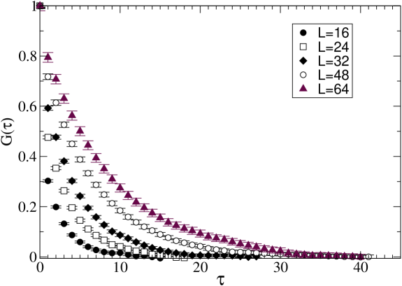
Figure 3: The auto-correlation function $G(t)$ is shown as a function of $t$ for $L=16,24,32,48$ and $64$

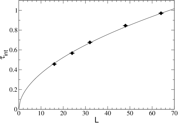
Figure 4: Integrated auto-correlation time as a function of $L$.

Here we estimate $\tau_{\rm int}$ for the chiral susceptibility. As we will see in the next section, $\xi$ is infinite for the parameters we use ($N=1,d=2,m=0$), since there are massless excitations. Hence, we study the behavior of $\tau_{\rm int}$ as a function of the lattice size $L$. Figure 3 plots the function $G(t)$ for $L=16,24,32,48$ and $64$. This graph suggests a simple choice for $t_{\rm max}$ for various $L$’s. We choose $t_{\rm max}=12,16,20,30,30$ for the five values of increasing $L$. This defines $\tau_{\rm int}$ uniquely. We plot the results in figure 4. The function $0.107L^{0.53}$ (solid line) roughly captures the behavior of $\tau_{\rm int}$ as a function of $L$ suggesting that the dynamical critical exponent $z$ of our algorithm is around $0.5$.

Let us now compare the directed-path algorithm discussed here with the Metropolis algorithm developed in a previous work Cha01 ; Cha02 . This is of interest since the results from the previous algorithm were quite unexpected and may be wrong. In the earlier work the two dimensional partition function was rewritten in terms of loop variables and the dimers along the loop were updated using a Metropolis accept-reject step. It was shown that the algorithm reproduced exact results with good precision on small lattices. Based on the evidence from the directed path algorithm, we now argue that the auto-correlation time of the previous algorithm grows uncontrollably for large lattices. In figure 5 we compare $4000$ consecutive measurements of the chiral susceptibility in the simulation time history at $m=0$ on a $32\times 32$ lattice, between the old and the new algorithms.

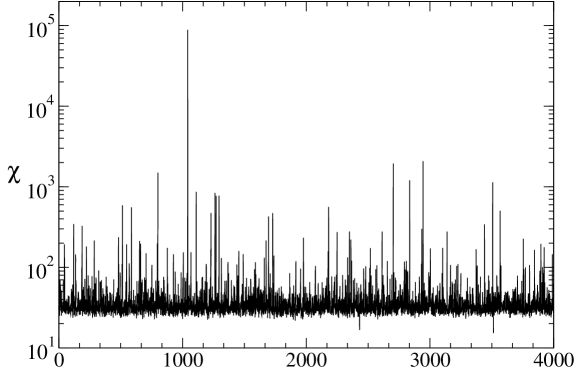
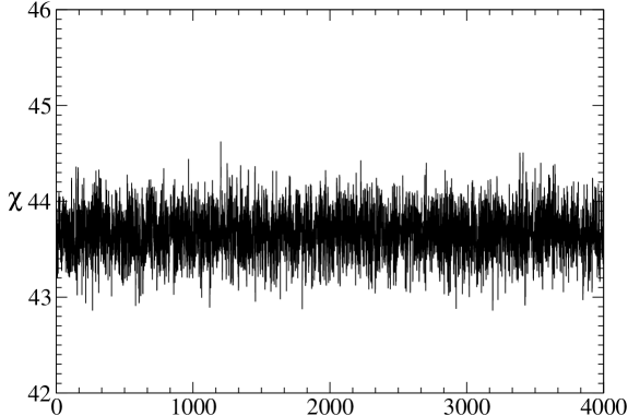
Figure 5: Comparison of simulation time histories of the chiral susceptibility for 4000 consecutive measurements between the old (top graph) and the new (bottom graph) algorithms for $L=32$.

In both cases, measurements are performed after a comparable amount of computer time. The fluctuations in the old algorithm are clearly much larger. The average of $300,000$ measurements with the old algorithm gives a value of $41.8(6)$ as compared to $43.669(5)$ obtained from just 4000 measurements with the new algorithm. This clearly demonstrates the efficiency of the new algorithm in addition to showing that the earlier algorithm underestimates the final answer. Note that there is one measurement of the order of $10^{5}$ visible in the old algorithm time history. If we remove this measurement from our analysis we obtain an answer of $41.0(2)$ even with $4000$ measurements. This is consistent with the value obtained by averaging over the entire time history. Without more statistics it would be impossible to say whether these spikes are isolated events or contribute an important fraction to the final answer. However, our new and more efficient algorithm shows us that the contributions from these isolated spikes are indeed important and can contribute up to five percent to the final answer on a $32\times 32$ lattice. Comparing the results obtained from the new and the old algorithms for different lattice sizes, we now believe that these large spikes contribute even a larger percentage to the final answer on larger lattices. Most likely the old algorithm is not able to tunnel between important sectors of the configuration space and develops large auto-correlation times at large volumes. Due to insufficient statistics we think that the contributions from the spikes were not sampled properly in the previous work and hence the final answers were systematically lower. This led to wrong conclusions.

VII RESULTS IN THE CHIRAL LIMIT

In this section we present some results obtained using the algorithm in the chiral limit. We focus on the issue of chiral symmetry breaking in various dimensions. As discussed earlier, the finite size scaling of the chiral susceptibility is an ideal observable for investigating this issue. All the results given below are obtained with $t=1$.

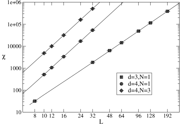
Figure 6: Finite size scaling of the Chiral Susceptibility in three and four dimensions. The solid lines represent fits of the data as described in the text.

Based on the work of Sal91 we know that at strong couplings chiral symmetry is broken in three and four dimensions. In figure 6 we plot the chiral susceptibility ($\chi$) as a function of the lattice size $L$ in $d=3,4$ when $N=1$ and in $d=4$ when $N=3$. For $d=4$ the data fits very well to the functional form $aL^{d}+b$, where $a$ and $b$ are constants. This functional form is motivated from chiral perturbation theory. In the case of $d=3$ chiral perturbation theory suggests a form $aL^{d}+bL^{4-d}+c$. Again the data fits well to this form over the entire range. The values of all the fit parameters and the $\chi^{2}/$d.o.f. obtained from the fits are given in table 3. The solid lines in figure 6 represent these fits.

Table 3:

N	d	a	b	c	$\chi^{2}$/d.o.f.
1	3	0.05493(5)	1.75(9)	-10(1)	0.5
1	4	0.05124(7)	3.6(2)	–	0.5
3	4	0.4823(2)	12(5)	–	0.2

The divergence of the susceptibility with $L$ is consistent with spontaneous breaking of chiral symmetry. Using eq.(14) we see that the infinite volume chiral condensate is given by $\langle\bar{\psi}\psi\rangle=\sqrt{a}$. We find

$$\langle\bar{\psi}\psi\rangle=\left\{\begin{array}[]{ccc}0.2343(2)&\mbox{for}&N=1,d=3\cr 0.2264(2)&\mbox{for}&N=1,d=4\cr 0.6945(3)&\mbox{for}&N=3,d=4.\end{array}\right.$$ (43)

We would like to remind the reader that the errors in the fitting parameters do not include all the systematic errors that arise due to variations in the analysis procedures.

In two dimensions the Mermin-Wagner-Coleman theorem forbids the formation of a condensate Mer66 ; Col73 . However, it is well known that a theory with $U(1)$ symmetry can still contain massless excitations. Of course there is always a possibility for the theory to be in the chirally symmetric massive phase. To which phase does our model at $t=1$ belong? The behavior of $\chi$ as a function of $L$ in both the possible phases was already discussed in eq.(14). In figure 7 we plot $\chi$ as a function of $L$ for $N=1,2,3,5,8,10,20$. We find that all of the shown data fit reasonably well to the function $\chi=aL^{2-\eta}$. The solid lines show these fits.

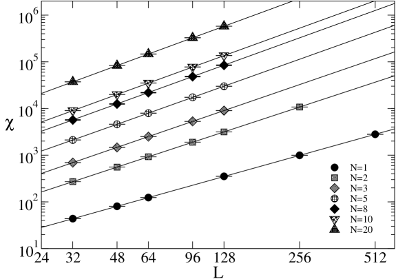
Figure 7: Finite size scaling of the Chiral Susceptibility in two dimensions for different values of $N$. The solid lines are fits as discussed in the text.

The values of $a,\eta$ and $\chi^{2}/$d.o.f. are given in table 4.

Table 4:

$N$	$a$	$\eta$	$\chi^{2}$/d.o.f.
1	0.239(1)	0.498(2)	1.2
2	0.586(1)	0.230(1)	1.6
3	1.139(3)	0.149(1)	2.7
5	2.78(1)	0.086(1)	0.11
8	6.71(2)	0.054(1)	0.28
10	10.22(5)	0.043(2)	0.33
20	39.1(2)	0.021(2)	0.64

This result strongly suggests that two dimensional staggered fermions at strong couplings are in the critical massless phase.

The partition function of two dimensional dimer models ($N=1$, no monomers) on a planar lattice can be solved exactly Kas63 ; Tem61 ; Fis61 . In Fis63 a determinant formula for the two monomer correlation function ($\langle\bar{\psi}\psi(x)\ \bar{\psi}\psi(y)\rangle$) was derived in the infinite lattice setting. A combination of analytic and numerical analysis in Fis63 provided strong evidence that this correlation function decays as $1/|x-y|^{1/2}$ when $|x-y|$ is large. This implies (in $N=1$ case) that the chiral susceptibility $\chi$ diverges as $L^{3/2}$ in large volumes, i.e. $\eta=0.5$. Our $N=1$ algorithm result $\eta=0.498(2)$ is in excellent agreement with this semi-exact result.

At the other extreme, a large $N$ analysis leads to the conclusion that chiral symmetry is spontaneously broken even in two dimensions. Then the condensate must be non-zero. How does the condensate acquire a non-zero value? A resolution to this paradox was proposed by Witten in Wit78 . He predicted that $\eta\sim c/N$ for large $N$, so that when $N$ is strictly infinite $\eta=0$ and $\chi\sim L^{2}$ as expected in a phase with broken chiral symmetry in two dimensions (see eq.(14)). Our data is consistent with this expectation. We find that all of our data fits well to the form $\eta=0.420(3)/N+0.078(4)/N^{2}$ with $\chi^{2}/{\rm d.o.f.}\sim 0.33$. Our data along with the fit is shown in figure 8. The $1/N^{2}$ term in the fitting function is necessary to fit the data for $N=1,2,3$.

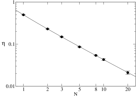
Figure 8: $\eta$ as a function of $N$. The solid line corresponds to the function $0.42/N+0.078/N^{2}$.

VIII CONCLUSIONS

In this article we have introduced a new type of cluster algorithm to update strongly coupled $U(N)$ lattice gauge theories with staggered fermions in the chiral limit. We studied the performance of the algorithm in two dimensions for a specific set of parameters and discovered that it has a dynamical critical exponent of roughly one half. We found the algorithm to be extremely efficient even in three and four dimensions. This progress allows us, for the first time, to study questions related to the chiral limit of a gauge theory beyond the mean field approximation.

As a first step we studied the question of chiral symmetry breaking. We used finite size scaling of the chiral susceptibility as a tool to address this question. We found clear evidence that the $U(1)$ chiral symmetry is spontaneously broken in three and four dimensions. On the other hand, in two dimensions we found that the theory contains massless excitations although the chiral condensate was zero. This is consistent with the Mermin-Wagner-Coleman theorem. The critical exponent $\eta=0.498(2)$ obtained with the algorithm for $N=1$ in two dimensions is in excellent agreement with the semi-exact result of $0.5$ inferred from Fis63 . Further, $\eta$ scales as $1/N$ for large $N$ as predicted in Wit78 .

We believe our algorithm can be useful in addressing some interesting physics questions. For example, the universality of the finite temperature QCD chiral phase transition with staggered fermions remains controversial Aok98 ; Ber00 . It would be useful to give a definitive answer at least at strong couplings. Previous calculations could only be performed far from the chiral limit and on small lattices Boy92 . Using our algorithm we can now settle this question completely. Another question of interest is to determine the critical density of baryons where chiral symmetry restoration takes place. At strong couplings and in the static approximation (heavy baryon limit) this question can be answered with our algorithm. Since baryons are known to be heavy at strong couplings this approximation may even be justifiable. Our algorithm can also be used to extract quantities like the decay width of the rho meson at strong couplings. This would be instructive since we would learn more about the difficulties involved in such calculations that are not merely algorithmic.

The present work also raises many interesting algorithmic questions. Can one extend our algorithm to other situations? For example, can one study more than one flavor of staggered fermions? This is interesting since one can then explore more complex chiral symmetry breaking patterns. Can Wilson fermions and Domain wall fermions be studied at strong couplings using similar techniques? Interesting and controversial phase structures have been predicted for the latter Gol00 ; Bro00 . What about a systematic way to go towards the weak coupling limit? Perhaps allowing a fermionic plaquette term in the Boltzmann weight already has some desirable effects. What about more general applications? For example it is possible to rewrite the determinant of a matrix as a sum over monomer-dimer configurations. Does this mean we can calculate the determinant of certain types of matrices more easily than before?

Finally, our algorithm should also be of interest to physicists studying monomer-dimer systems. Such systems are interesting in their own right and have a long history Hei72 . Many statistical mechanics problems including the Ising model can be reformulated in terms of monomer-dimer models on various kinds of lattices. Novel Monte Carlo algorithms continue to be developed to study them Kra02 . We believe that our approach can provide a useful alternative.

Acknowledgments

We would like to thank Pierre van Baal, Wolfgang Bietenholz, Peter Hasenfratz, Ferenc Niedermayer, Costas Strouthos and Uwe-Jens Wiese for helpful comments. S.C. would also like thank U.-J. Wiese for hospitality during S.C.’s visit to Bern University where a major part of this work was done. This work was supported in part by funds provided by the U.S. Department of Energy grant DE-FG02-96ER40945. D.A. is supported at Leiden by a Marie Curie fellowship from the European Commission (contract HPMF-CT-2002-01716). The computations were performed on CHAMP, (a 64-node Computer-cluster for Hadronic and Many-body Physics), funded by the Department of Energy and the Intel Corporation and located in the physics department at Duke University.

Appendix A DERIVATION OF EXPRESSIONS FOR OBSERVABLES

Here we present a brief derivation of the relations (33) and (34). We begin by noting that the chiral condensate is given by

$$\langle\bar{\psi}\psi(x)\rangle=\frac{1}{Z(m)}\,\sum_{[{}n,b]_{x}}\,W([{}n,b]_{x})\,m^{n}$$ (44)

where the sum is over monomer-dimer configurations $[n,b]_{x}$ which satisfy the usual constraint relation (6) on all sites except the site $x$ where the relation is modified to

$$n_{x}+\sum_{\mu}b_{\mu}(x)+b_{-\mu}(x)=N-1.$$ (45)

The partition function on the other hand is given by

$$Z(m)\ =\ \sum_{[{}n,b]}\,W([{}n,b]_{x})\,m^{n}$$ (46)

where the sum is over monomer-dimer configurations $[n,b]$ which satisfy the usual constraint on all sites. The weights $W([n,b]_{x})$ and $W([n,b])$ appearing in (44) and (46) are obtained by multiplying the block weights (16) and (17) associated to all active and passive blocks. Since the mass is not taken into account in these weights we have an extra factor $m^{n}$ where $n$ refers to the total number of monomers in the configuration.

Let us now construct an update to go from a given configuration $[n^{\prime},b^{\prime}]_{x}$ to a configuration $[n,b]$. This update is performed as follows:

1. We declare the site $x$ to be passive.

2. We start at the site $x$ and choose the first bond to be one of the $2d$ bonds. The probability to choose the $\mu=\pm 1$ bond is given by $t^{2}/(2d-2+2t^{2})$ and the probability to choose one of the $\mu\neq\pm 1$ bond by $1/(2d-2+2t^{2})$.

3. Once we pick the bond we increase the dimer content of that link by one and go to the adjoint active block.

4. We then use the probabilities discussed in section III to construct a directed path update which ends on some active site $y$.

Let the path generated using the above rules be referred to as $\alpha_{xy}$. At the end of the above update it is easy to prove that the new configuration belongs to the type $[n,b]$. Let $P([n^{\prime},b^{\prime}]_{x};\alpha_{xy})$ refer to the probability to produce the path $\alpha_{xy}$ starting from the configuration $[n^{\prime},b^{\prime}]_{x}$ using this update.

Now consider the unique reverse path of $\alpha_{xy}$ referred to as $\alpha^{-1}_{xy}$. This path is one of the “partial” directed paths that we produce using the directed path algorithm described in section III. In particular this path is a path that starts from the active site $y$ and visits the passive block at $x$. Let $P([n,b];\alpha^{-1}_{xy})$ be the probability of generating this reverse path using the algorithm. Since the forward and reverse paths are produced by probabilities that satisfy detailed balance at each stage except for possible factors at the ends, it is easy to argue that

$$P([n^{\prime},b^{\prime}]_{x};\alpha_{xy})\ W([n^{\prime},b^{\prime}]_{x})\ m^{n^{\prime}}=\frac{VNm}{(2d-2+2t^{2})}\ P([n,b];\alpha^{-1}_{xy})\ W([n,b])\ m^{n}$$ (47)

The factor $V$ arises because the site $y$ is picked with probability $1/V$ but not the site $x$. The factor $N$ is due to the uncanceled factor from (30). The factor $1/(2d-2+2t^{2})$ compensates the same factor from the left hand side. The mass factor arises because of the mismatch in the number of monomers between the two configurations; in particular $n^{\prime}=n+1$.

Now by construction we know

$$\sum_{\{\alpha_{xy}\}}P([n^{\prime},b^{\prime}]_{x};\alpha_{xy})=1$$ (48)

where the sum is over all possible paths $\alpha_{xy}$. These paths always start at the same $x$ but end at various sites $y$. Thus we derive the relation

$$W([n^{\prime},b^{\prime}]_{x})m^{n^{\prime}}=\sum_{\{\alpha_{xy}\}}\frac{VNm}{(2d-2+2t^{2})}P([n,b];\alpha^{-1}_{xy})\ W([n,b])m^{n}$$ (49)

where the configurations $[n,b]$ on the right hand are determined from the configuration $[n^{\prime},b^{\prime}]_{x}$ and the path $\alpha_{xy}$. It is then possible to argue that

$$\sum_{[n^{\prime},b^{\prime}]_{x}}W([n^{\prime},b^{\prime}]_{x})m^{n^{\prime}}=\sum_{[n,b]}\sum_{\{\alpha^{-1}_{xy}\}}\frac{VNm}{(2d-2+2t^{2})}\ P([n,b];\alpha^{-1}_{yx})W([n,b])m^{n}.$$ (50)

Since the directed path update produces paths $\alpha^{-1}_{xy}$ starting from the configuration $[n,b]$ with probability $P([n,b];\alpha^{-1}_{xy})$, we see that

$$\frac{1}{V}\langle\bar{\psi}\psi(x)\rangle=\frac{mN}{2d-2+2t^{2}}\Big{\langle}\sum_{y}I(x,y)\Big{\rangle}$$ (51)

where $I(x,y)$ was defined in section IV and the average on the right hand side is taken over the ensemble of configurations generated in the directed path algorithm. This proves relation (33).

In order to show (34) we start with the relation (49) and assume that the mass factors are site dependent. By differentiating the relation (49) with respect to the mass factor at the site $y$ we can generate weights of configurations that contribute to the two monomer correlations. This then yields (34). We leave the steps of this derivation to the reader.

Appendix B EXACT RESULTS ON SMALL LATTICES

In this appendix we give explicit expressions for the coefficients $c_{2n}$ defined in eq. (38), as a function of $x=t^{2}$ for a selection of small lattice sizes and small values of $N$ where exact calculations are possible.

B.1 $N=1$ on a $2\times 2$ lattice

$$c_{0} = 4(1+x^{2})$$

$$c_{2} = 4(1+x)$$

$$c_{4} = 1$$

B.2 $N=1$ on a $2\times 2\times 2$ lattice

$$c_{0} = 16(4+4x^{2}+x^{4})$$

$$c_{2} = 8(16+16x+8x^{2}+4x^{3})$$

$$c_{4} = 4(20+16x+6x^{2})$$

$$c_{6} = 2(8+4x)$$

$$c_{8} = 1$$

B.3 $N=1$ on a $4\times 4$ lattice

$$c_{0} = 16(1+4x^{2}+7x^{4}+4x^{6}+x^{8})$$

$$c_{2} = 64(2+4x+10x^{2}+13x^{3}+13x^{4}+10x^{5}+4x^{6}+2x^{7})$$

$$c_{4} = 32(13+40x+81x^{2}+96x^{3}+81x^{4}+40x^{5}+13x^{6})$$

$$c_{6} = 64(11+37x+63x^{2}+37x^{4}+11x^{5})$$

$$c_{8} = 8(83+256x+354x^{2}+256x^{3}+83x^{4})$$

$$c_{10} = 32(11+28x+28x^{2}+11x^{3})$$

$$c_{12} = 8(13+24x+13x^{2})$$

$$c_{14} = 16(1+x)$$

$$c_{16} = 1$$

B.4 $N=2$ on a $2\times 2\times 2$ lattice

$$c_{0} = 1156+3136x^{2}+2116x^{4}+576x^{6}+81x^{8}$$

$$c_{2} = 16(476+784x+1064x^{2}+870x^{3}+502x^{4}+264x^{5}+72x^{6}+27x^{7})$$

$$c_{4} = 4(4428+8512x+9532x^{2}+6624x^{3}+3302x^{4}+1056x^{5}+243x^{6})$$

$$c_{6} = 16(1132+2116x+1976x^{2}+1116x^{3}+386x^{4}+75x^{5})$$

$$c_{8} = 2(4714+7744x+5768x^{2}+2304x^{3}+443x^{4})$$

$$c_{10} = 16(166+220x+116x^{2}+25x^{3})$$

$$c_{12} = 12(34+32x+9x^{2})$$

$$c_{14} = 16(2+x)$$

$$c_{16} = 1$$

B.5 $N=1$ on a $4\times 2\times 2$ lattice

$$c_{0} = 16(256+256x^{2}+112x^{4}+16x^{6}+x^{8})$$

$$c_{2} = 128(128+128x+160x^{2}+104x^{3}+52x^{4}+20x^{5}+4x^{6}+x^{7})$$

$$c_{4} = 32(832+1280x+1296x^{2}+768x^{3}+324x^{4}+80x^{5}+13x^{6})$$

$$c_{6} = 64(352+592x+504x^{2}+252x^{3}+74x^{4}+11x^{5})$$

$$c_{8} = 8(1328+2048x+1416x^{2}+512x^{3}+83x^{4})$$

$$c_{10} = 32(88+112x+56x^{2}+11x^{3})$$

$$c_{12} = 8(52+48x+13x^{2})$$

$$c_{14} = 16(2+x)$$

$$c_{16} = 1$$

B.6 $N=1$ on a $2\times 2\times 4$ lattice

$$c_{0} = 16(81+232x^{2}+216x^{4}+96x^{6}+16x^{8})$$

$$c_{2} = 128(63+98x+142x^{2}+130x^{3}+84x^{4}+56x^{5}+16x^{6}+8x^{7})$$

$$c_{4} = 32(563+1064x+1242x^{2}+944x^{3}+532x^{4}+192x^{5}+56x^{6})$$

$$c_{6} = 64(284+529x+512x^{2}+312x^{3}+120x^{4}+28x^{5})$$

$$c_{8} = 8(1179+1936x+1492x^{2}+640x^{3}+140x^{4})$$

$$c_{10} = 32(83+110x+60x^{2}+14x^{3})$$

$$c_{12} = 8(51+48x+14x^{2})$$

$$c_{14} = 16(2+x)$$

$$c_{16} = 1$$

B.7 $N=2$ on a $4\times 4$ lattice

$$c_{0} = 65536(81+576x^{2}+2416x^{4}+5648x^{6}+7520x^{8}+5648x^{10}$$

$$+2416x^{12}+576x^{14}+81x^{16})$$

$$c_{2} = 2097152(54+144x+564x^{2}+1145x^{3}+2490x^{4}+3806x^{5}$$

$$+5470x^{6}+6303x^{7}+6303x^{8}+5470x^{9}+3806x^{10}+2490x^{11}$$

$$+1145x^{12}+564x^{13}+144x^{14}+54x^{15})$$

B.8 $N=3$ on a $2\times 2\times 2$ lattice

$$c_{0} = {\textstyle\frac{1}{81}}(4624+25600x^{2}+35396x^{4}+20224x^{6}+5800x^{8}+900x^{10}+81x^{12})$$

$$c_{2} = {\textstyle\frac{2}{27}}(10880+25600x+54080x^{2}+63556x^{3}+62912x^{4}+47560x^{5}$$ (52)

$$+28220x^{6}+15120x^{7}+5620x^{8}+2220x^{9}+450x^{10}+135x^{11})$$

B.9 $N=2$ on a $4\times 2\times 2$ lattice

$$c_{0} = 1336336+3625216x^{2}+5242816x^{4}+3817024x^{6}+1491668x^{8}$$

$$+318272x^{10}+37072x^{12}+2304x^{14}+81x^{16}$$

$$c_{2} = 64(275128+453152x+1053864x^{2}+1260996x^{3}+1522636x^{4}$$ (53)

$$+1299408x^{5}+1009344x^{6}+630309x^{7}+334475x^{8}+154496x^{9}$$

$$+56066x^{10}+19137x^{11}+4508x^{12}+1128x^{13}$$

$$+144x^{14}+27x^{15})$$

B.10 $N=2$ on a $2\times 2\times 4$ lattice

$$c_{0} = 198916+1682272x^{2}+4177396x^{4}+4825728x^{6}$$

$$+3184704x^{8}+1343232x^{10}+381996x^{12}+69984x^{14}+6561x^{16}$$

$$c_{2} = 32(140936+399424x+11511968x^{2}+1787069x^{3}+2560377x^{4}$$ (54)

$$+2707684x^{5}+2511784x^{6}+2002594x^{7}+1320438x^{8}+840288x^{9}$$

$$+403668x^{10}+212841x^{11}+70956x^{12}+31590x^{13}+5832x^{14}$$

$$+2187x^{15})$$

B.11 $N=1$ on a $2\times 2\times 2\times 2$ lattice

$$c_{0} = 256(81+124x^{2}+54x^{4}+12x^{6}+x^{8})$$

$$c_{2} = 128(792+968x+936x^{2}+600x^{3}+240x^{4}$$

$$+144x^{5}+24x^{6}+8x^{7})$$

References

- (1) For recent review of this problem see C. Bernard et. al., Nucl. Phys. Proc. Suppl.106, 199 (2002).
- (2) C. Bernard et. al., arXiv: hep-lat/0209086
- (3) M. Lüscher, Nucl. Phys. B364, 237 (1991).
- (4) J.-M. Drouffe and J.-B. Zuber, Phys. Rept. 102, (1983) 1.
- (5) N.Kawamoto and J. Smit Nucl.Phys.B192:100,1981
- (6) H. Kluberg-Stern, A. Morel and B. Petersson, Nucl.Phys.B215:527,1983
- (7) P. Rossi and U. Wolff, Nucl. Phys. B248, 105 (1984).
- (8) F. Karsch and H. Mütter, Nucl. Phys. B313, 541 (1989).
- (9) R. Aloisio et. al., Nucl. Phys. B564 (2000) 489.
- (10) S. Chandrasekharan, Phys. Lett. B536, 72 (2002).
- (11) S. Chandrasekharan, eprint arXiv: hep-lat/0208071.
- (12) G. Boyd et. al., Nucl. Phys. B376 (1992) 199.
- (13) N.D. Mermin and H. Wagner, Phys. Rev. Lett.17: (1966) 1133.
- (14) S. Coleman, Comm. Math. Phys. 31 (1973) 259.
- (15) H. Evertz, G. Lana and M. Marcu, Phys. Rev. Lett. 70 (1993) 875.
- (16) O. F. Syljuasen and A. W. Sandvik, Phys. Rev. E66, 046701 (2002).
- (17) R. Brower, S.Chandrasekharan and U.-J. Wiese, Physica A261, (1998) 520.
- (18) S. Chandrasekharan, Nucl. Phys. (Proc.Suppl.) 83 (2000) 774.
- (19) U. Wolff, Phys. Lett. B228 (1989) 379.
- (20) M. Salmhofer, E. Seiler, Commun.Math.Phys.139 (1991) 395, Erratum-ibid.146 (1992) 637.
- (21) E. Witten, Nucl. Phys. B145 (1978) 110.
- (22) P.W. Kasteleyn, J. Math. Phys. 4 (1963) 287.
- (23) H.N.V. Temperley and M.E. Fisher, Phil. Mag. 6 (1961) 1061.
- (24) M.E. Fisher, Phys. Rev. 124 (1961) 1664.
- (25) M.E. Fisher and J. Stephenson, Phys. Rev. 63 (1963) 1411.
- (26) S. Hashimoto et.al., eprint arXiv: hep-lat/0209091.
- (27) S.Aoki et. al., Phys. Rev. D57 (1998) 3910.
- (28) C. Bernard et. al.,Phys. Rev. D61 (2000) 054503.
- (29) M. Golterman and Y. Shamir, JHEP 0009 (2000) 006.
- (30) R. Brower and B. Svetitsky, Phys. Rev. D61 (2000) 114511.
- (31) O. J. Heilmann and E. H. Lieb, Comm. Math. Phys. 25 (1972) 190.
- (32) W. Krauth and R. Moessner, arXiv:cond-mat/0206177.