Dynamical fermions as a global correction

Abstract

In the simplified setting of the Schwinger model we present a systematic study on the simulation of dynamical fermions by global accept/reject steps that take into account the fermion determinant. A family of exact algorithms is developed, which combine stochastic estimates of the determinant ratio with the exploitation of some exact extremal eigenvalues of the generalized problem defined by the ‘old’ and the ‘new’ Dirac operator. In this way an acceptable acceptance rate is achieved with large proposed steps and over a wide range of couplings and masses.

1 Introduction

The problem to include fermionic fluctuations in QCD simulations has been in the focus of interest of the lattice community for a long time. An overview over the standard approaches to such simulations can be found in [1]. About the most obvious idea that one may have, is the following succession of steps: First we propose changes of the gauge field by some efficient algorithm that fulfills detailed balance with respect to some suitable pure gauge action. Then we add a Metropolis accept/reject step. This correction has to filter the ensemble such that it becomes governed by the desired action including the fermion determinant, whose change enters the accept decision. Since the proposal is not guided by the fermions, one may however fear to get sufficient acceptance only for tiny rather local changes of the gauge field and to get an overall very inefficient algorithm by a succession of such steps. Alternative approaches, including the presently most popular hybrid Monte Carlo algorithm [2, 3] (HMC), therefore use some sort of stochastic representation of fermion effects to guide the gauge field evolution at the expense of introducing additional noise and having to make many small and expensive steps involving inversions of the Dirac operator.

While fermionic guidance may prove indispensable for many lattice simulations, in our opinion there is also some interest to pursue the direct Metropolis approach. One reason is the growing interest in Dirac operators, where the fermions are coupled to smoothed SU(3)-projected averages of the fundamental gauge fields [4, 5, 6, 7, 8]. Here the dependence of the operators on the fundamental fields to be updated becomes so complicated, that their change even under infinitesimal moves, which leads to the fermionic force, becomes impracticable to evaluate both on paper and CPU. Metropolis on the other hand requires nothing but a routine that is able to apply the Dirac operator to given fields. A similar situation prevails with Ginsparg Wilson fermions, for instance in the form of the overlap formulation [9].

An additional important motivation for the present investigation stems for us from our interest in simulations of the Schrödinger functional with dynamical fermions [10, 11]. Here one is also interested in larger $\beta$-values implying small physical volume and approximate validity of perturbation theory. Then we expect fluctuations of the determinant to become a small (one-loop) effect. Our future hope is to develop a Metropolis algorithm for the determinant whose efficiency in the large $\beta$ limit becomes more similar to pure gauge simulations based on hybrid overrelaxation. HMC-type algorithms on the other hand remain rather costly also in this limit. If such an algorithm can be constructed, it will be interesting to see, if and where there is a cross-over in efficiency compared to HMC.

Reliable algorithmic optimizations with dynamical fermions in four dimensional theories are very costly and large scale projects by themselves. Therefore — like other researchers — we decided to first undertake a study in two-dimensional QED, the Schwinger model [12, 13, 14, 15]. This simplification allows for clean clinical tests using for instance the precise knowledge of the full spectrum of fermionic operators. We are of course aware of the risk, that the smoother gauge fields in this superrenormalizable model may teach us lessons that do not carry over to QCD. Therefore we plan to soon test the algorithms derived here in the four dimensional Schrödinger functional.

Other efforts to use the determinant directly in Metroplis steps have been reported in [16] for Wilson fermions and in [17] for staggered fermions with blocked links. In [18] a hierarchical system of acceptance steps has been tested. Although interesting, we think it is fair to say that none of these projects has led to a strong competitor for HMC for standard actions to date.

Our two dimensional study presented here is organized as follows. In section 2 we set up the notation and our lattice formulation of the Schwinger model. In section 3 we investigate the behavior of the global Metropolis algorithm with determinants evaluated exactly. Our main result is contained in section 4 where the stochastic estimation of determinants is introduced together with a new class of partially stochastic updates, which is tested in a number of applications in section 5. After conclusions two appendices follow where we derive exact formulas for the acceptance rate as a function of the eigenvalues in an associated generalized eigenvalue problem. The perturbative solution of this problem is discussed in appendix B.

2 Model laboratory

In this section we introduce our formulation of the Schwinger model discretized as two dimensional noncompact U(1) gaugefields and Wilson fermions. Quenched gaugefields are generated by a global heatbath. We work in lattice units setting the lattice spacing $a=1$.

2.1 Formulation of the path integral

Gauge potentials $A_{\mu}(x)$ are taken as the primary fields which are integrated over all real values. In terms of the field strength

$$F_{\mu\nu}=\Delta_{\mu}A_{\nu}-\Delta_{\nu}A_{\mu},$$ (2.1)

where $\Delta_{\mu}$ is the forward difference, the gauge action reads

$$S_{G}[A]=\frac{1}{4}\sum_{x\mu\nu}F_{\mu\nu}^{2}$$ (2.2)

with $\mu,\nu=0,1$. A well-defined path integral on a finite torus of length $L$ yields the pure gauge partition function

$$Z_{G}=\int DA\prod_{\mu}\delta(\sum_{x}A_{\mu})\prod_{x}\delta(\Delta_{\mu}^{*}A_{\mu})\exp(-S_{G}[A]),$$ (2.3)

where $\Delta_{\mu}^{*}$ means the backward difference and $DA=\prod_{x\mu}dA_{\mu}(x)$. The $\delta$-functions fix all modes that do not receive damping by $S_{G}$. In addition to the gauge degrees of freedom these are two modes corresponding to constant shifts of $A_{\mu}$ that we shall come back to. For later use we abbreviate the normalized full gauge measure as

$$D\mu(A)=\frac{1}{Z_{G}}DA\,\prod_{\mu}\delta(\sum_{x}A_{\mu})\prod_{x}\delta(\Delta_{\mu}^{*}A_{\mu})\exp(-S_{G}[A])$$ (2.4)

and the gauge average as

$$\langle X(A)\rangle_{G}=\int D\mu(A)X(A).$$ (2.5)

To couple fermions to $A_{\mu}(x)$ in a gauge invariant fashion we choose a coupling strength $g$ and form phases

$$U_{\mu}(x)=\exp(igA_{\mu}(x))$$ (2.6)

and covariant difference operators

$$D_{\mu}f(x) = U_{\mu}(x)f(x+\hat{\mu})-f(x)$$ (2.7)

$$D^{*}_{\mu}f(x) = f(x)-U^{*}_{\mu}(x-\hat{\mu})f(x-\hat{\mu}).$$ (2.8)

Now the Wilson operator reads

$$D_{W}=\sum_{\mu}\frac{1}{2}\left\{\gamma_{\mu}(D_{\mu}+D^{*}_{\mu})-D^{*}_{\mu}D_{\mu}\right\}$$ (2.9)

with some choice of hermitian $\gamma$ matrices. In terms of

$$\gamma_{5}=i\gamma_{0}\gamma_{1}$$ (2.10)

we have the pseudo-hermiticity property

$$D_{W}^{\dagger}=\gamma_{5}D_{W}\gamma_{5}\,.$$ (2.11)

For our algorithmic study we choose periodic boundary conditions for the fields that $D_{W}$ acts on. Had we allowed constant components in $A_{\mu}$ then we could transform them away by a non-periodic gauge transformation. This would however modify the fermion boundary conditions by extra phase factors. Our constraint may thus be viewed as a definite set of boundary conditions in imposing a finite volume.

The partition function for $N_{f}$ flavours of mass $m$ is taken as

$$Z=\int D\mu(A)\det(D_{W}+m)^{N_{f}}.$$ (2.12)

In the following we restrict ourselves to the strictly positive case $N_{f}=2$ analogous to QCD with only light degenerate flavours.

Wilson loops constructed from the phases $U_{\mu}$ decay in the gauge ensemble with an exact area law. The string tension

$$\sigma=\frac{g^{2}}{2}$$ (2.13)

is used to eliminate the dimensionful coupling $g$ in favour of the dimensionless combination

$$z=\sqrt{\sigma}L\,.$$ (2.14)

In the pure gauge theory the limit $L\to\infty$ at fixed $z$ corresponds to a continuum limit at finite physical volume.

2.2 Generation of gauge fields

Gauge fields distributed with $D\mu(A)$ can be generated by a global heatbath procedure or independent sampling. A potential $A$ in the Markov chain is followed by $A^{\prime}$ which, due to the constraints, can be written as

$$A^{\prime}_{\mu}=\epsilon_{\mu\nu}\Delta_{\nu}^{*}\phi.$$ (2.15)

The lattice scalar $\phi$ is taken as the Fourier transform

$$\phi(x)=\frac{1}{L}\sum_{p}\tilde{\phi}(p)\exp(ip\cdot x).$$ (2.16)

of independent Gaussian random numbers $\tilde{\phi}(p)$

$$\tilde{\phi}(0)=0,\quad\tilde{\phi}^{*}(p)=\tilde{\phi}(-p)$$ (2.17)

$$\langle\,\tilde{\phi}^{*}(p)\,\tilde{\phi}(q)\,\rangle=\frac{1}{(\hat{p}^{2})^{2}}\delta_{pq}\quad(p\not=0).$$ (2.18)

Momenta are summed over the appropriate Brillouin zone and $\tilde{\phi}$ depends on them periodically.

It will also be of interest for us to mimic smaller update moves $A\to A^{\prime\prime}$ which are not independent but just fulfill detailed balance with respect to $S_{G}$. This can be achieved by taking

$$A^{\prime\prime}=cA+sA^{\prime}\,,\quad c=\cos(t\pi/2),\,s=\sin(t\pi/2),$$ (2.19)

where the parameter $0<t\leq 1$ allows to control the step-size.

In Fig.1 a few complete spectra of the Wilson Dirac operator are shown for several couplings at $L=8$ in gauge fields generated according to (2.4). The high degeneracy of the free spectrum is progressively lifted as $z$ is raised. At the same time the spectrum moves away from the origin.

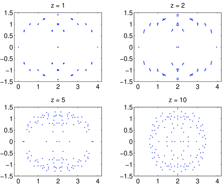
Figure 1: Typical spectra of $D_{W}$ at couplings $z=1,2,5,10$

For each configuration we define an effective critical mass $m_{0}$ to be the negative spectral gap

$$m_{0}(A)=-\min[\mbox{Re}({\rm spec}(D_{W}))]$$ (2.20)

such that the smallest real part of all eigenvalues of $D_{W}+m_{0}$ just reaches zero. Its gauge average is taken as a critical value

$$m_{c}(z,L)=\langle m_{0}(A)\rangle_{G}$$ (2.21)

and by $\sigma_{c}^{2}(z,L)$ we denote the corresponding variance.

	$L=8$		$L=12$		$L=16$
z	$m_{c}/g^{2}$	$\sigma_{c}/g^{2}$	$m_{c}/g^{2}$	$\sigma_{c}/g^{2}$	$m_{c}/g^{2}$	$\sigma_{c}/g^{2}$
$1$	-0.323(3)	0.088	-0.382(3)	0.082	-0.427(3)	0.086
$2$	-0.314(3)	0.086	-0.379(3)	0.084	-0.420(3)	0.081
$5$	-0.289(2)	0.071	-0.353(2)	0.068	-0.391(2)	0.069
$10$	-0.169(1)	0.020	-0.262(2)	0.028	-0.319(1)	0.031

Table 1: Values for the critical mass and its standard deviation from 1000 configurations each.

In Table 1 some numerical values are listed. We divide by $g^{2}$ as suggested by perturbation theory and obtain numbers that vary only slowly with $L$ and $z$. For the spectra in Fig.1 this implies gaps roughly proportional to $z^{2}$ in agreement with the four particular configurations shown. In our algorithmic study we find it appropriate to use these data to choose mass values such that our fermions are light and thus dynamically relevant, but heavy enough to not suffer from the ‘exceptional’ unphysical modes known to occur with Wilson fermions.

3 Metropolis with exact determinants

In this section we use a rather ideal fermion algorithm that is only available in our two-dimensional model: global heatbath proposals with respect to the gauge action filtered through a Metropolis step based on the exact fermionic determinant. With the cost of computing the determinant by standard linear algebra means scaling like $L^{3D}$ this appears prohibitive beyond $D=2$. Here on the other hand it will prove to be quite feasible up to medium size lattices and will provide a rigorous upper bound for the acceptance rates achievable with stochastic techniques.

3.1 Exact acceptance rate

In equilibrium for the ensemble (2.12) the acceptance rate $q$ for proposals with the pure gauge global heatbath described in the previous section is given by

$$q=\frac{1}{Z}\int D\mu(A)|\det(D_{W}+m)|^{2}\int D\mu(A^{\prime})\min\left(1,\frac{|\det(D^{\prime}_{W}+m)|^{2}}{|\det(D_{W}+m)|^{2}}\right),$$ (3.1)

where $A$ and $A^{\prime}$ enter into $D_{W}$ and $D^{\prime}_{W}$. In a more symmetric form this reads

$$q = \frac{1}{Z}\int D\mu(A)\int D\mu(A^{\prime})\min\left(|\det(D_{W}+m)|^{2},|\det(D^{\prime}_{W}+m)|^{2}\right)$$ (3.2)

$$= 1-\frac{\int D\mu(A)\int D\mu(A^{\prime})\left||\det(D_{W}+m)|^{2}-|\det(D^{\prime}_{W}+m)|^{2}\right|}{\int D\mu(A)\int D\mu(A^{\prime})\left(|\det(D_{W}+m)|^{2}+|\det(D^{\prime}_{W}+m)|^{2}\right)},$$

and $q$ clearly obeys $0\leq q\leq 1$. Any nontrivial dependence of the determinant on the gaugefield reduces the acceptance.

To estimate $q$ we generate a large number of $N$ independent gaugefields with the pure gauge measure and compute the fermion determinant for each of them. Let $d_{i},i=1,\ldots,N$ be the resulting successive values of $|\det(D_{W}+m)|^{2})$. Then $q$ may be estimated by

$$q\approx\frac{\frac{1}{N(N-1)}\sum_{i\not=j}\min(d_{i},d_{j})}{\frac{1}{N}\sum_{i}d_{i}}.$$ (3.3)

For larger $N$-values the double sum is best evaluated by using a sorting algorithm (with cost only $\propto N\ln(N)$, see [19], for instance provided in Matlab),

$$\{d^{<}_{i}\}={\rm sort}(\{d_{i}\}),$$ (3.4)

where the sequence $\{d^{<}_{i}\}$ consists of the same members as $\{d_{i}\}$ but reordered such that $d^{<}_{1}\leq d^{<}_{2}\leq\ldots\leq d^{<}_{N}$. Now the acceptance is written as

$$q\approx\frac{\sum_{i}w_{i}d^{<}_{i}}{\sum_{i}d^{<}_{i}}$$ (3.5)

with the weights

$$w_{i}=\frac{2(N-i)}{(N-1)}\,.$$ (3.6)

For the error estimation one of course has to take into account that the O($N^{2}$) terms in the numerator of (3.3) that are effectively summed by (3.5) are not independent.

It turns out to be very successful to make a Gaussian model for the distribution of the fermionic action in the gauge ensemble

$$\nu(E)=<\delta(E-S_{F})>_{G},\quad S_{F}=-2\log(|\det(D_{W}+m)|),$$ (3.7)

by setting

$$\nu(E)=\frac{1}{\sqrt{2\pi}\Sigma}\exp\left(\frac{-(E-E_{0})^{2}}{2\Sigma^{2}}\right).$$ (3.8)

Once this Ansatz has been made, its free parameters $E_{0}$ and, more important, $\Sigma$ can also be estimated numerically from the observed values $d_{i}$ by determining mean and variance of $S_{F}$. Within the model the acceptance rate then follows,

$$q=2\,\frac{\int_{-\infty}^{+\infty}dE\,\nu(E)\exp(-E)\int_{-\infty}^{E}dE^{\prime}\,\nu(E^{\prime})}{\int_{-\infty}^{+\infty}dE\,\nu(E)\exp(-E)}\,.$$ (3.9)

With the expression (3.8) for $\nu$ one sees that $q$ is independent of $E_{0}$ as it should (irrelevance of a constant in $S_{F}$). It is convenient to extract $q$ from the distribution $\tilde{\nu}(\Delta)$ for the energy difference $\Delta=E^{\prime}-E$

$$\tilde{\nu}(\Delta)=\frac{1}{Z}\int_{-\infty}^{+\infty}dE\,\nu(E)\exp(-E)\int_{\infty}^{+\infty}dE^{\prime}\,\nu(E^{\prime})\,\delta(\Delta-E^{\prime}+E)$$ (3.10)

with

$$Z=\int_{-\infty}^{+\infty}dE\;\nu(E)\exp(-E),$$ (3.11)

for which we obtain

$$\tilde{\nu}(\Delta)=\frac{1}{2\sqrt{\pi}\Sigma}\exp\left(-\frac{1}{4\Sigma^{2}}(\Delta-\Sigma^{2})^{2}\right).$$ (3.12)

In terms of $\tilde{\nu}$ we evaluate

$$q=\int_{-\infty}^{+\infty}d\Delta\;\tilde{\nu}(\Delta)\min(1,\exp(-\Delta))=\frac{2}{\sqrt{\pi}}\int_{\Sigma/2}^{\infty}du\exp(-u^{2})={\rm erfc}(\Sigma/2).$$ (3.13)

We performed a series of (quenched) simulations on $L=8,12,16$ lattices with $z=1,2,5,10$ (compare Table 1) where we determined and stored the complete spectra of $D_{W}$. These data may be used to construct fermion determinants and acceptance rates for a whole range of masses and in this fashion we produce Fig.2.

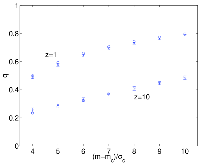
Figure 2: Acceptance rates versus mass for $L=16$. Numerical values from (3.5) are shown as crosses and circles correspond to the model using (3.13) with the observed $\Sigma$.

It demonstrates that in our model, at least with the exact fermion determinant, a simulation based on global Metropolis steps is feasible over a wide range of masses. Note that this even refers here to maximally large quenched gauge move proposals. Moreover we verify the validity of the Gaussian model (circles).

3.2 Enhanced acceptance rate

So far we have considered the generation of potentials with the pure gauge action $S_{G}$ and the incorporation of the determinant in an accept/reject step. The same ensemble may also be produced by a different split of the total action and it is conceivable that this leads to an enhanced acceptance rate. It corresponds to a simple version of ultraviolet filtering [18, 20, 21] by modifying the fermion action just by the plaquette term. Apart from the gauge action contained in the measure $D\mu(A)$ we include another component

$$Z=\int D\mu(A)\exp[(1-\alpha^{2})S_{G}]|\det(D_{W}+m)|^{2}$$ (3.14)

which in simulations is combined with the determinant in the Metropolis test. By rescaling $A_{\mu}$ one easily sees that this ensemble is equivalent to the standard form of the gauge action with an effective coupling of strength $g/\alpha$ in (2.6). Whenever the highest acceptance, for fixed $g/\alpha$, is reached at $\alpha\not=1$ the extra term has enhanced the acceptance and is hence advantageous.

In simulations we perform the expensive evaluation of the determinant with one fixed value of $g$ in (2.6) and then compute the acceptance for many values $\alpha$ in the additional term. In this way we construct lines in a graph of $q$ versus $z$, where $z$ refers to the effective coupling. With a number of such lines, we shall see which one gives the highest acceptance for a $z$ at which we wish to simulate.

The Gaussian model generalizes by assuming a joint Gaussian distribution for $S_{G},S_{F}$ with a $2\times 2$ covariance matrix given by connected correlations

$$<S_{G}S_{G}>_{G}^{c} = v_{GG}=\frac{1}{2}(L^{2}-1)$$ (3.15)

$$<S_{F}S_{F}>_{G}^{c} = v_{FF}$$ (3.16)

$$<S_{G}S_{F}>_{G}^{c} = v_{GF}=v_{FG}\,,$$ (3.17)

of which the first one is trivial due to the Gaussian gauge action.

Instead of $S_{F}$ alone, acceptance is now controlled by the combination $E=S_{F}+(\alpha^{2}-1)S_{G}$ whose variance $\Sigma^{2}$, given by

$$\Sigma^{2}=(\alpha^{2}-1)^{2}v_{GG}+v_{FF}+2(\alpha^{2}-1)v_{GF}$$ (3.18)

may now be used in (3.13) to estimate $q$. Within the model, we can easily vary $\alpha$ continuously.

In Fig.3 we see a number of approximate acceptance trajectories constructed in this way for $L=16,m=-0.1$. For each of them 1000 gauge configurations were used and exponentiated in the determinants with coupling $\bar{z}$ corresponding to the crosses. The parameter $\alpha$ within the Gaussian model was then varied in the interval $[0.8,1.2]$ producing the acceptance trajectories as functions of $z=\bar{z}/\alpha$. We clearly see that ultraviolet filtering pays off. At weak coupling the acceptance is high without it, and correspondingly less can be gained.

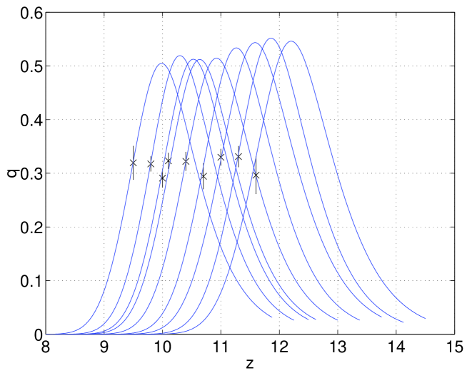
Figure 3: Enhanced acceptance rate in the Gaussian model for $L=16,m=-0.1$. The crosses correspond to $\alpha=1$. Each of them extends to a curve according to (3.13), (3.18), as $\alpha$ is varied in the interval $[0.8,1.2]$.

For the case with the cross at $\bar{z}=10$ we now confront the Gaussian predictions for the $\alpha$-dependence of $q$ with numerical values as in (3.3) where now $d_{i}=\exp[-S_{F}-(\alpha^{2}-1)S_{G}]$ enters. This is shown in Fig.4 for an ensemble of 1000 gauge potentials and confirms the model also in this more general setting.

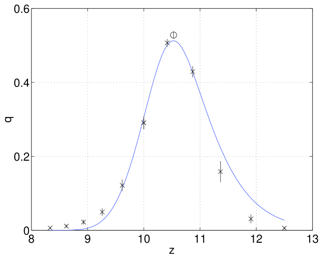
Figure 4: Acceptance rates for $L=16,m=-0.1$. The curve corresponds to the Gaussian model based on the simulation $\bar{z}=10$, other data with errors are direct Monte Carlo checks. The circle is at $\alpha=0.950$ that minimizes (3.18).

4 Partially stochastic global acceptance steps

Metropolis steps based on the availability of exact fermion determinant ratios are of conceptual interest but hardly lead to efficient algorithms on large lattices and in four dimensions. An approximate stochastic estimation that nevertheless maintains exact detailed balance can be defined and at first seems more promising [17, 22, 23]. We found however that this can easily lead to negligibly small acceptance at smaller masses. Therefore we developed a more general Metropolis correction step based on an only partially stochastic estimation of determinant changes (PSD) which is complemented by a few exact eigenvalues [see [24] for related ideas in connection with reweighting corrections to the polynomial hybrid Monte Carlo algorithm]. In this section we shall thus derive a family of (exact) algorithms which contains those based on exact and on fully stochastic determinants as extremal cases between which we interpolate.

4.1 Stochastic estimation of fermion determinant ratios

The stochastic estimation of the determinant reduces the problem to solving linear equations with the fermion matrix at the expense of statistical errors on top of the main Monte Carlo process. The fundamental formula is

$$\int D[\eta]\rho(M\eta)=|\det(M)|^{-2}.$$ (4.1)

Here we integrate over a complex valued spinor field with the measure

$$D[\eta]=\prod_{x\alpha}\frac{d\mbox{Re}(\eta)d\mbox{Im}(\eta)}{\pi}$$ (4.2)

for each site $x$ and spinor component $\alpha$. For the normalized probability distribution $\rho$,

$$\int D[\eta]\rho(\eta)=1$$ (4.3)

we often take a Gaussian

$$\rho(\eta)=\exp\left[-\eta^{\dagger}\eta\right]\,,$$ (4.4)

but keep the formulas more general where we can. The determinant appears as a Jacobian in (4.1) for arbitrary $\rho$. We may also write an unbiased estimate of the determinant as

$$|\det(M)|^{-2}=\left<\frac{\rho(M\eta)}{\rho(\eta)}\right>_{\eta}$$ (4.5)

with an average $<.>_{\eta}$ over the random field $\eta$ only.

For an acceptance step from a given field $A$ to a proposed new $A^{\prime}$ with associated operators $D_{W},D_{W}^{\prime}$ we now form the “ratio operator”

$$M=(D_{W}^{\prime}+m)^{-1}(D_{W}+m),$$ (4.6)

and in terms of this matrix we could stochastically accept with the probability

$$w_{0}(A,A^{\prime})=\min[1,\rho(M\eta)/\rho(\eta)]\,,$$ (4.7)

where the dependence on $\eta$ and the choice of $\rho$ is left implicit. For the reverse transition, $A\leftrightarrow A^{\prime}$, we find $M\leftrightarrow M^{-1}$. Therefore

$$\frac{\left<w_{0}(A,A^{\prime})\right>_{\eta}}{\left<w_{0}(A^{\prime},A)\right>_{\eta}}=\frac{\int D[\eta]\min[\rho(\eta),\rho(M\eta)]}{\int D[\eta]\min[\rho(\eta),\rho(M^{-1}\eta)]}=|\det(M)|^{-2}$$ (4.8)

shows detailed balance. The last equality follows by changing variables $\eta\to M\eta$ in the integral in the numerator. These steps constitute the fully stochastic algorithm that we are going to generalize to PSD.

The acceptance rate is always smaller than (3.1) due to the inequality

$$\int D[\eta]\min[\rho(\eta),\rho(M\eta)] \leq \min\left[\int D[\eta]\rho(\eta),\int D[\eta]\rho(M\eta)\right]$$ (4.9)

$$= \min(1,|\det(M)|^{-2})$$

Hence, the exact acceptance rate in this context is something like the ideal “Carnot” efficiency which we cannot reach but which we may also not want to miss by too much. The question may arise, if the acceptance rate may be increased by averaging over several random $\eta$ fields. If we average under the $\min$ function, $N_{\eta}=1$ seems to be the only finite value for which detailed balance can be shown. Averaging outside of $\min$ seems correct but would not raise the average acceptance.

An expression for the stochastic acceptance rate with distribution $\rho$ is given in analogy to (3.1) by the integral

$$q_{0} = \frac{1}{Z}\int D\mu(A)|\det(D_{W}+m)|^{2}\int D\mu(A^{\prime})\;\langle w_{0}(A,A^{\prime})\rangle_{\eta}$$

$$= \frac{1}{Z}\int D\mu(A)|\det(D_{W}+m)|^{2}\int D\mu(A^{\prime})\int D[\eta]\min[\rho(\eta),\rho(M\eta)]$$

$$= \frac{1}{Z}\int D\mu(A)\int D\mu(A^{\prime})\int D[\eta]\min[\rho((D_{W}+m)^{-1}\eta),\rho((D^{\prime}_{W}+m)^{-1}\eta)]$$

A naive Monte Carlo estimation of the last expression for $q_{0}$ with $\rho=\exp(-\eta^{\dagger}\eta)$ is not practical due to the very strong fluctuations of the integrand. We shall however be able to perform the $\eta$-integrations exactly in this case, which may be viewed as the construction of an improved estimator (same mean value, smaller variance) for $q_{0}$ in terms of generalized eigenvalues.

We work out the dependence of

$$\langle w_{0}\rangle_{\eta}=\int D[\eta]\min[\rho(\eta),\rho(M\eta)]$$ (4.11)

on the spectrum $\{\lambda_{i}\}$ of $M^{\dagger}M$ with $i=1,\ldots,n=2L^{2}$ for the choice $\rho=\exp(-\eta^{\dagger}\eta)$. Performing the above integration in the basis of orthonormal eigenvectors of $M^{\dagger}M$ with components $z_{i}$ we find

$$\langle w_{0}\rangle_{\eta}=\prod_{i}\left(\int\frac{d\mbox{Re}z_{i}d\mbox{Im}z_{i}}{\pi}\right)\min\left[\exp(-\sum_{i}|z_{i}|^{2})\,,\,\exp(-\sum_{i}\lambda_{i}|z_{i}|^{2})\right].$$ (4.12)

Changing to polar variables in all the complex planes we get

$$\langle w_{0}\rangle_{\eta}=\prod_{i}\left(\int_{0}^{\infty}du_{i}\right)\min\left[\exp(-\sum_{i}u_{i})\,,\,\exp(-\sum_{i}\lambda_{i}u_{i})\right].$$ (4.13)

In appendix A this integral is evaluated exactly yielding

$$\langle w_{0}\rangle_{\eta}=\sum_{i}\;\min(1,1/\lambda_{i})\prod_{j\not=i}\;\frac{\lambda_{i}-1}{\lambda_{i}-\lambda_{j}}\,,$$ (4.14)

where the special case of $S$ being the empty set suffices here (compare (A.1)).

It is clear from (4.13) that eigenvalues $\lambda_{i}=1$ are irrelevant for the acceptance. Approaching this limit for one of them in (4.14) one indeed finds it to drop out and one is left with the formula for $n-1$ eigenvalues. If we now consider as an example the case of $\lambda_{2}\ldots\lambda_{n-1}$ differing from one only negligibly and only one remaining pair with $\lambda_{n}\gg 1>\lambda_{1}$ then we find a small acceptance

$$\langle w_{0}\rangle_{\eta}\approx\frac{2-\lambda_{1}}{\lambda_{n}}\,.$$ (4.15)

It remains small even for $\lambda_{1}\lambda_{n}=1=\det(M^{\dagger}M)$, when we have 100% non-stochastic acceptance. This simple example demonstrates how the stochastic acceptance rate degrades if a determinant ratio of order unity arises from compensations between the eigenvalues of the squared ratio operator $M^{\dagger}M$. We are hence motivated to have a closer look at such spectra in our model.

4.2 Spectrum of random quotients of Dirac operators

In practice we find the spectrum $\{\lambda_{i}\}$ of $M^{\dagger}M$ by solving the generalized eigenvalue problem

$$(D_{W}+m)(D_{W}+m)^{\dagger}\chi=\lambda(D_{W}^{\prime}+m)(D_{W}^{\prime}+m)^{\dagger}\chi\,.$$ (4.16)

A general observation about the spectrum of $M^{\dagger}M$, at least for not too strong coupling, is that there are two low and two high almost degenerate eigenvalues separated from the remaining ones. In the bulk of the spectrum the eigenvalues are close to one which is easy to understand, since all eigenvalues would be exactly one if the two gaugefields entering into $M$ would be equal.

A few experiments show that the separation of the extremal eigenvalues becomes more pronounced as the mass is lowered. In the same limit and at small coupling they are of the order $g^{2}$ and $g^{-2}$ respectively.

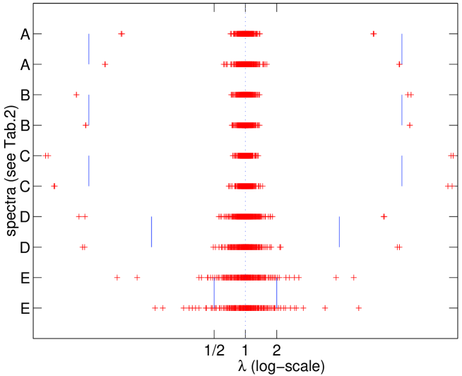
Figure 5: Typical complete generalized spectra $\{\lambda_{i}\}$ for values $m,z$ found in Tab.2. Vertical bars show the scales $g^{2}$ and $g^{-2}$.

This is illustrated in Fig.5 by the example of the quenched spectra on $L=8$ for several combinations $m,z$. They are labelled by A–E with the corresponding values contained in Tab.2. in Sect. 5.1. The plot shows the complete generalized spectra on a logarithmic scale. For the spectra labelled by A–D one clearly sees that the bulk is between 1/2 and 2 with two eigenvalues close to $g^{2},g^{-2}$ on either side, while for the more strongly coupled case E this segregation is lost.

To understand how such a spectrum arises, we consider two hermitian operators $H$ and $H^{\prime}$ and the generalized Ritz functional (or Rayleigh quotient)

$$\mu(\psi)=\frac{\psi^{\dagger}H\psi}{\psi^{\dagger}H^{\prime}\psi}\,.$$ (4.17)

The vectors $\psi_{\star}$ for which $\mu(\psi)$ is stationary satisfy the generalized eigenvalue equation $H\psi_{\star}=\lambda H^{\prime}\psi_{\star}$ with $\lambda=\mu(\psi_{\star})$. In particular the smallest generalized eigenvalue $\lambda_{\rm min}$ has the property

$$\mu(\psi)\geq\lambda_{\rm min}\quad\mbox{for all $\psi$}\,.$$ (4.18)

In our case $H=(D_{W}+m)(D_{W}+m)^{\dagger}$ and $H^{\prime}=(D_{W}^{\prime}+m)(D_{W}^{\prime}+m)^{\dagger}$. The typical situation is encountered if we set $m=0$ and assume that $H$ and $H^{\prime}$ are positive for nonvanishing coupling (note that $m_{c}<0$).

Instead of considering directly the generalized eigenvalue problem (4.16) we use the relation $H=D_{W}D_{W}^{\dagger}=(D_{W}\gamma_{5})^{2}$ and first study the spectrum

$$D_{W}\gamma_{5}\,\psi=\kappa\psi$$ (4.19)

in perturbation theory. By expanding $U_{\mu}=1+igA_{\mu}-g^{2}A_{\mu}^{2}/2+\mathcal{O}(g^{3})$ we obtain an expansion of the Wilson Dirac operator

$$D_{W}=(D_{W}^{(0)}+gD_{W}^{(1)}+g^{2}D_{W}^{(2)}+\mbox{\rm O}(g^{3}))\,.$$ (4.20)

We are interested in the perturbation of the eigenvalue $\kappa^{(0)}=0$ of the free operator $D_{W}^{(0)}\gamma_{5}$. It is doubly degenerate with spatially constant free eigenfunctions $\psi_{\pm}^{(0)}$. We set up expansions

$$\kappa_{\alpha} = g\kappa^{(1)}_{\alpha}+g^{2}\kappa^{(2)}_{\alpha}+\mbox{\rm O}(g^{3})\,,$$ (4.21)

$$\psi_{\alpha} = \psi^{(0)}_{\alpha}+g\psi^{(1)}_{\alpha}+g^{2}\psi^{(2)}_{\alpha}+\mathcal{O}(g^{3})\,,\quad\alpha=1,2\,.$$ (4.22)

The perturbation $D_{W}^{(1)}$ is proportional $A_{\mu}(x)$ which has no zero momentum component. Hence matrix elements of this operator vanish between states of equal momentum and in particular between $\psi_{\pm}^{(0)}$. This implies the vanishing of $\kappa^{(1)}_{\alpha}$. Suitable zeroth order eigenfunctions $\psi^{(0)}_{\alpha}$ are linear combinations of $\psi_{\pm}^{(0)}$ which we determine later. The first order equation for the eigenvectors is

$$D_{W}^{(0)}\gamma_{5}\psi_{\alpha}^{(1)}=-D_{W}^{(1)}\gamma_{5}\psi_{\alpha}^{(0)}\,,\quad\alpha=1,2\,.$$ (4.23)

In second order the $2\times 2$ matrix

$$\psi^{(0)}_{k}\left[D_{W}^{(2)}-D_{W}^{(1)}D_{W}^{(0)-1}D_{W}^{(1)}\right]\gamma_{5}\psi^{(0)}_{l}\,,\quad k,l=\pm\,$$ (4.24)

has to be diagonalized. Here the eigenvectors $\psi^{(0)}_{\alpha}$ get determined together with eigenvalues $\kappa^{(2)}_{\alpha}$ which lift the degeneracy.

Now we consider the Ritz functional $\mu(\psi)$ (4.17) setting $\psi$ equal to $\psi_{\alpha}=\psi^{(0)}_{\alpha}+g\psi^{(1)}_{\alpha}+\mbox{\rm O}(g^{2})$. Using the relation (4.23) we get

$$\psi_{\alpha}^{\dagger}D_{W}D_{W}^{\dagger}\psi_{\alpha} = (\kappa_{\alpha}^{(2)})^{2}g^{4}+\mbox{\rm O}(g^{5})\,,$$ (4.25)

$$\psi_{\alpha}^{\dagger}D_{W}^{\prime}D_{W}^{\prime\dagger}\psi_{\alpha} = \psi_{\alpha}^{(0)\dagger}[(D_{W}^{(1)}-D_{W}^{\prime(1)})\gamma_{5}]^{2}\psi_{\alpha}^{(0)}g^{2}+\mbox{\rm O}(g^{3})\,.$$ (4.26)

From (4.18) we derive an upper bound for the minimal generalized eigenvalue $\lambda_{\rm min}$ of (4.16)

$$\lambda_{\rm min}\leq{\rm const}\times g^{2}\quad(m=0)\,.$$ (4.27)

By considering the inverse Ritz functional $\mu^{-1}(\psi)$ and setting $\psi$ equal to the eigenfunctions $\psi_{\alpha}^{\prime}$ of $D_{W}^{\prime}\gamma_{5}$ we can derive in full analogy to the above a lower bound for the maximal generalized eigenvalue $\lambda_{\rm max}$ of (4.16)

$$\lambda_{\rm max}\geq{\rm const}^{\prime}\times g^{-2}\quad(m=0)\,.$$ (4.28)

A detailed analysis of the perturbation expansion of the generalized eigenvalues themselves, which confirms the variational arguments given here, is deferred to appendix B.

4.3 Partially stochastic estimation of determinant ratios

We saw that a few extremal eigenvalues in $M^{\dagger}M$ can ruin the stochastic acceptance rate even if the relevant determinant ratio is close to unity. Moreover, at least in our model, these kind of spectra are really common. We now develop a mixed strategy treating the bulk of the eigenvalues stochastically and a few special ones exactly. Of course, detailed balance has now to be demonstrated for the combination. For the time being we content ourselves with proofs for $\rho(\eta)=\exp(-\eta^{\dagger}\eta)$ only. More general cases may well be possible.

We assume, that for each spectrum we can identify a set $S$ such that $\{\lambda_{i}|i\in S\}$ consists of the $s=|S|$ extremal eigenvalues of $M^{\dagger}M$ (the same number of large and small ones), which we treat deterministically. The associated eigenvectors $\{\phi_{i}|i\in S\}$, that we choose to be orthonormal, span an $s$ dimensional subspace that we characterize by a projection operator

$$P=\sum_{i\in S}\phi_{i}\;\phi_{i}^{\dagger}\equiv P(A,A^{\prime})$$ (4.29)

Here we remind ourselves that $P$, via the Dirac operators $D_{W},D_{W}^{\prime}$, depends on a pair of gauge potentials $A,A^{\prime}$. Due to the symmetric inclusion of large and small $\lambda_{i}$ a spectral analysis of the inverse operator $(M^{\dagger}M)^{-1}$ with inverted eigenvalues would lead to the same projector (for the same $M$).

Anticipating a discussion of detailed balance we are interested in information about the relation between $P(A,A^{\prime})$ and $P(A^{\prime},A)$. As mentioned before, going to the reverse process ($A\leftrightarrow A^{\prime}$), $M$ changes to $M^{-1}$. Hence in this case we are concerned with the eigenvalue problem of $M^{-1{\dagger}}M^{-1}=(MM^{\dagger})^{-1}$. Its eigenvalues are reciprocal to those of $M^{\dagger}M$ but the eigenvectors and hence the associated projectors are different, $P(A^{\prime},A)\not=P(A,A^{\prime})$. The problems are however related by a unitary transformation

$$MM^{\dagger}=U^{\dagger}M^{\dagger}MU,\quad U^{\dagger}U=1=UU^{\dagger}\,.$$ (4.30)

Explicitly, U may be written as

$$U=M^{\dagger}(MM^{\dagger})^{-1/2}\,.$$ (4.31)

The same unitary transformation relates the eigenvectors of the two problems such that

$$P(A^{\prime},A)=U^{\dagger}P(A,A^{\prime})U\,.$$ (4.32)

holds.

Returning to the forward problem we can factorize

$$M^{\dagger}M=(\bar{P}+PM^{\dagger}M)(P+\bar{P}M^{\dagger}M)$$ (4.33)

where we introduced the complementary projector

$$\bar{P}=1-P$$ (4.34)

and used standard properties of projectors and commutativity $PM^{\dagger}M=M^{\dagger}MP$, which is easily seen in the spectral representation of $M^{\dagger}M$. While both factors in (4.33) are nonsingular operators in the full domain, they have a block structure with unit operators in the subspaces of $\bar{P}$ and $P$. The exact “small” determinant of the first factor is

$$\det(\bar{P}+PM^{\dagger}M)=\prod_{i\in S}\lambda_{i}.$$ (4.35)

A stochastic estimator for an acceptance step with the second factor alone would be given by (see (4.7))

$$\min\left[1,\exp(-\eta^{\dagger}\bar{P}(M^{\dagger}M-1)\bar{P}\eta)\right]\;.$$

As the true partially stochastic acceptance criterion $w_{s}(A,A^{\prime})$ to accept a proposed $A^{\prime}$ given an ‘old’ $A$ we now propose

$$w_{s}(A,A^{\prime})=\min\left[1,\prod_{i\in S}\lambda_{i}^{-1}\exp(-\eta^{\dagger}\bar{P}(M^{\dagger}M-1)\bar{P}\eta)\right]$$ (4.36)

To prove detailed balance we start from

$$w_{s}(A^{\prime},A)=\min\left[1,\prod_{i\in S}\lambda_{i}\exp(-\eta^{\dagger}U^{\dagger}\bar{P}U((MM^{\dagger})^{-1}-1)U^{\dagger}\bar{P}U\eta)\right]\,.$$ (4.37)

In

$$\langle w_{s}(A^{\prime},A)\rangle_{\eta}=$$ (4.38)

$$\int D[\eta]\min\left[\exp(-\eta^{\dagger}\eta),\prod_{i\in S}\lambda_{i}\exp(-\eta^{\dagger}U^{\dagger}(P+\bar{P}(M^{\dagger}M)^{-1})U\eta)\right]$$

a change of variables

$$\eta=U^{\dagger}(P+\bar{P}M^{\dagger}M)^{1/2}\eta^{\prime}$$ (4.39)

yields the desired result

$$\frac{\langle w_{s}(A,A^{\prime})\rangle_{\eta}}{\langle w_{s}(A^{\prime},A)\rangle_{\eta}}=\prod_{i\in S}\lambda_{i}^{-1}\det(P+\bar{P}M^{\dagger}M)^{-1}=|\det(M)|^{-2}\,.$$ (4.40)

With the above formalism we have an algorithm which avoids the low stochastic acceptance from extremal eigenvalues if their product is of order unity. It remains to discuss how to compute the required eigenvalues and -vectors. We do not attempt a detailed discussion here. An obvious idea is however to generalize the method used by the ALPHA collaboration in the past to obtain low and high lying eigenvectors of the ordinary problem. It is based on minimizing a Ritz functional by a conjugate gradient technique [26]. The relevant functional for the generalized problem is

$$\mu(\chi)=\frac{|(D_{W}+m)\chi|^{2}}{|(D_{W}^{\prime}+m)\chi|^{2}}$$ (4.41)

This functional is extremal at generalized eigenvectors and its value there is one of the generalized eigenvalues which coincide with those of $M^{\dagger}M$. Different generalized eigenvectors $\chi_{i}$ are not orthogonal, but one may show that $\chi_{i}^{\dagger}(D_{W}+m)(D_{W}+m)^{\dagger}\chi_{j}=0$ if $\lambda_{i}\not=\lambda_{j}$. In fact, $(D_{W}+m)^{\dagger}\chi_{i}$ are the (unnormalized) eigenvectors of $M^{\dagger}M$ and $(D_{W}^{\prime}+m)^{\dagger}\chi_{i}$ are those of $MM^{\dagger}$. After finding the absolute minimum of $\mu$ at $\chi_{1}$ one may then search for the minimum in the space orthogonal to $(D_{W}+m)(D_{W}+m)^{\dagger}\chi_{1}$ to find $\chi_{2}$ belonging to the second smallest eigenvalue $\lambda_{2}$. For the largest eigenvalues one may proceed analogously or just exchange numerator and denominator of $\mu$. Note, that we do not need a solver during the minimization, that is no intolerable nested iterations. A solver is needed however in the stochastic part to apply $M$ or $M^{\dagger}M$ to $\bar{P}\eta$. Due to the filtering of the random vector through the projector this should however be a well-conditioned problem and take few iterations. An alternative method to construct the required eigenvalues and vectors could be Lanczos techniques [27] which are known to first converge for the extremal eigenvectors needed here.

5 Numerical experiments with PSD

5.1 Acceptance rate for PSD

We now consider the partially stochastic acceptance rate

$$q_{s}=\frac{1}{Z}\int D\mu(A)|\det(D_{W}+m)|^{2}\int D\mu(A^{\prime})\;\langle w_{s}\rangle_{\eta}\,.$$ (5.1)

The ‘observable’ $\langle w_{s}\rangle_{\eta}$ in this double pathintegral depends on the generalized eigenvalues $\lambda_{i}$ and on their division into the deterministic subset $S$ and the stochastic one $\bar{S}$. As limiting cases it includes the fully deterministic and fully stochastic evaluation. For a numerical estimation of $q_{s}$ we produce pairs of configurations $A_{k},A_{k}^{\prime}$ and determine for all of them, at some value of $z$, $d_{k}=|\det(D_{W}+m)|^{2}$, generalized eigenvalues $\lambda_{i}$ and from them estimates $a_{k}=\langle w_{s}\rangle_{\eta}$ according to (A.1, A.16). Then we have the Monte Carlo estimate

$$q_{s}\approx\frac{\sum_{k}d_{k}a_{k}}{\sum_{k}d_{k}}\,.$$ (5.2)

In Fig.6 it is shown how the average acceptance rises if starting from the fully stochastic case $s=0$ more and more eigenvalues are included in $S$. Parameters are $L=8,z=1,m=0.0125$ and 1000 pairs of configurations are sampled.

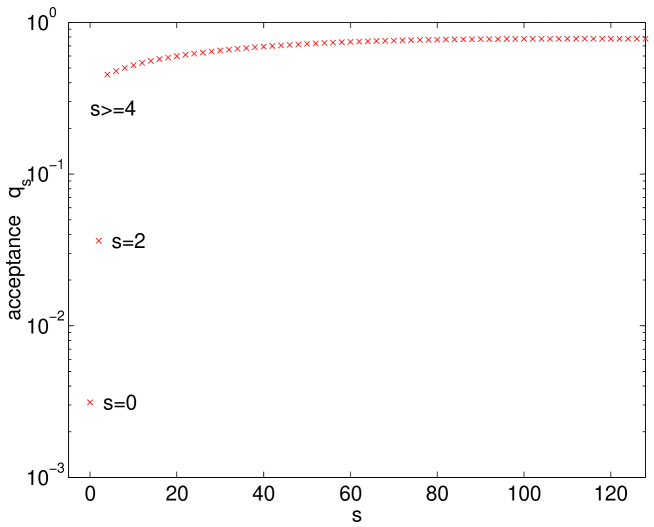
Figure 6: The acceptance rate vs. the number $s$ of nonstochastic generalized eigenvalues (parameters B in Tab.2).

Some further examples can be found in Tab.2.

$L$	$z$	$~{}~{}~{}m$	$~{}~{}~{}~{}q$	$~{}~{}~{}q_{0}$	$~{}~{}~{}q_{4}$	label
8	1	0.0250	0.837(7)	0.0141(2)	0.460(4)	A
8	1	0.0125	0.734(11)	0.0029(1)	0.425(6)	B
8	1	0.0050	0.602(15)	0.00061(2)	0.368(8)	C
8	2	0.0125	0.634(14)	0.0020(1)	0.130(3)	D
8	4	0.035	0.819(8)	0.00084(4)	0.0083(2)	E

Table 2: Values for acceptance rates for the deterministic ($q$), stochastic ($q_{0}$) and mixed case ($q_{4}$) with four extremal eigenvalues in $S$.

We note that there is a roundoff problem in the straightforward evaluation of (A.16) due to cancellations and significance loss. With standard double precision accuracy some clever recombination of terms would be required before using the formula much beyond $L=8$ with $n=128$ eigenvalues $\lambda_{i}$.

At this point we also study the dependence of the acceptances on the ‘size’ of the proposed moves. Global heatbath steps with respect to the gauge action that we have used so far are of maximal size. Lowering from one the parameter $t$ that we have introduced in (2.19) allows us to mimic smaller steps.

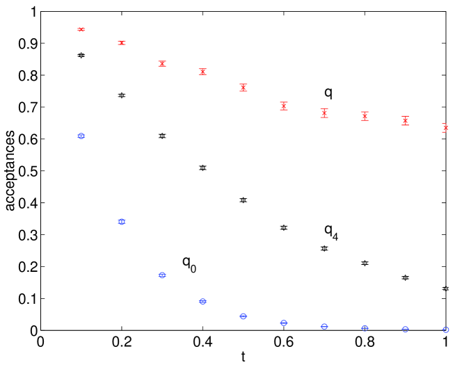
Figure 7: Acceptances rates versus stepsize $t$ for $L=8,m=0.0125,z=2$.

In Fig.7 we see the expected dependence of the acceptances. In particular we see that partially stochastic acceptance steps allow for much larger moves without excessive rejections.

Also in the partially stochastic case we have found a successful Gaussian model for the acceptance rate. Our starting point here is (5.1) which we break into two steps

$$\tilde{\nu}_{s}(\Delta)=\langle\langle\;\langle\,\delta[\Delta-\sum_{i\in S}\ln\lambda_{i}-\eta^{\dagger}\bar{P}(M^{\dagger}M-1)\eta]\,\rangle_{\eta}\;\rangle\rangle$$ (5.3)

with

$$\langle\langle{\cal O}\rangle\rangle=\frac{1}{Z}\int D\mu(A)|\det(D_{W}+m)|^{2}\int D\mu(A^{\prime})\,{\cal O}$$ (5.4)

and

$$q_{s}=\int_{-\infty}^{+\infty}d\Delta\,\tilde{\nu}_{s}(\Delta)\,\min(1,\exp(-\Delta)).$$ (5.5)

As a model we assume $\tilde{\nu}_{s}(\Delta)$ to be a Gaussian of mean $m_{s}$ and width $b_{s}$. For it $q_{s}$ evaluates to

$$q_{s}=\frac{1}{2}\,{\rm erfc}\left(\frac{m_{s}}{\sqrt{2}b_{s}}\right)+\frac{1}{2}\,{\rm erfc}\left(\frac{b_{s}^{2}-m_{s}}{\sqrt{2}b_{s}}\right)\exp(b_{s}^{2}/2-m_{s})\,.$$ (5.6)

In the expressions for the mean and width of the $\Delta$ distribution the $\eta$ integrations can be performed and we find

$$m_{s} = \langle\langle\,\sum_{i\in S}\ln\lambda_{i}+\sum_{i\in\bar{S}}(\lambda_{i}-1)\,\rangle\rangle$$ (5.7)

$$b_{s}^{2} = \langle\langle\,[\,\sum_{i\in S}\ln\lambda_{i}+\sum_{i\in\bar{S}}(\lambda_{i}-1)\,]^{2}\,\rangle\rangle-m_{s}^{2}+\langle\langle\,\sum_{i\in\bar{S}}(\lambda_{i}-1)^{2}\,\rangle\rangle.$$ (5.8)

In Tab.2 the last column is replaced by (0.452,0.419,0.364,0.140) in the Gaussian model for A–D, while the agreement is worse for case E with its different pattern of fluctuating eigenvalues.

5.2 The relevance of gaugefixing

We now turn to the question of gauge fixing. Up to now all gaugefields were generated in one and the same completely fixed gauge according to (2.4). Stochastic acceptance steps depend on the operator $M$ of (4.6). If only $\rho(\eta)$ is invariant under $x$-dependent phase transformations of the random field $\eta(x)$ then all acceptances are invariant under a change of gauge, that is the same transformation applied to $A$ and $A^{\prime}$. If however the update proposal includes a more or less random gauge move of $A^{\prime}$ relative to $A$, this is equivalent to only gauge transforming $A^{\prime}$. In this case the nonstochastic acceptance probability involving the ratio of gauge invariant determinants as in (3.1) is unchanged. This is however not true for the eigenvalues $\lambda_{i}$ of $M^{\dagger}M$ and of the generalized eigenvalue problem (4.16). We looked at the generalized spectrum for pairs $A_{\mu},A^{\prime}_{\mu}+\Delta_{\mu}\gamma$ for fixed $A,A^{\prime}$ and a number of randomly chosen gauge functions $\gamma(x)$. For nonvanishing $\gamma$ the eigenvalues $\lambda_{i}$ show much more variation and smaller values of $F(\lambda_{i})$ in (A.1) result while the ratio of determinants $\prod_{i}\lambda_{i}$ remains unchanged as it has to.

A non gauge-fixed simulation is achieved by replacing in (2.4)

$$\prod_{x}\delta(\Delta_{\mu}^{*}A_{\mu})\to\exp\left(-\frac{1}{2\xi^{2}}\sum_{x}(\Delta_{\mu}^{*}A_{\mu})^{2}\right)$$ (5.9)

such that the value $\xi=0$ corresponds to the previous case. It is not difficult to show that a global heatbath step for this measure is effected by a gaugefixed step as before followed by a gauge transformation with a gauge function $\gamma=\xi\phi$. Here a new independent random field $\phi$ is produced obeying (2.17, 2.18). Acceptance rates as functions of the gauge parameter are shown in Fig.8.

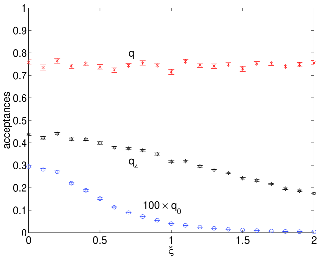
Figure 8: Acceptance rates versus gauge parameter $\xi$ for $L=8,m=0.0125,z=1$.

We notice the dramatic decay of the already small purely stochastic acceptance.

5.3 Some unquenched simulations with PSD

As a practical application we performed a few simulations on lattices $L=24$ with $z=1$ and $m=0$. By looking at Tab.1 we observe that for this value of $z$ the value of $\sigma_{c}/g^{2}$ seems to depend only weakly on $L$ whereas $-m_{c}/g^{2}$ increases monotonically with $L$. We have good reasons to expect that at these parameters no ‘exceptional’ fields with zero eigenvalues of the Wilson operator $D_{W}+m$ are proposed.

We compare PSD simulations at $s=4$ with exact determinants (equivalent to $s=2L^{2}$). At $s=4$ we employ both global heatbath ($t=1$) proposals and smaller update moves with the parameter t in (2.19) set to $1/2$. We measure the ‘pion’-susceptibility in the unquenched ensemble

$$\chi=\frac{1}{L^{2}}\,\left\langle\mbox{Tr}\left[D_{W}^{-1\,{\dagger}}D_{W}^{-1}\right]\right\rangle\,,$$ (5.10)

where Tr refers to both Dirac indices and space. Before integrating out the Grassmann valued fermion fields $\chi$ can also be interpreted as a susceptibility of the density $\bar{\psi}_{i}(x)\gamma_{5}\psi_{j}(x)$ for two flavors $\psi_{i},i=1,2$. We take $\chi$ here as a simple correlation function with significant contributions at the scale of the meson correlation length.

$s$	$t$	$q_{s}$	$\chi$(12)	$\tau_{{\rm int},\chi}$
$2L^{2}$	1	0.61	983(12)	2.4(3)
4	1	0.24	1005(15)	4.4(8)
4	1/2	0.50	997(14)	3.8(5)

Table 3: Results from simulations of 4900 measurements each on $L=24$ lattices with $z=1$ and $m=0$.

In Tab.3 we list our results for the acceptance rates and the susceptibility $\chi$ together with its integrated autocorrelation time $\tau_{\rm int,\chi}$, which is in units of (global) gaugefield updates. The stepsizes $t=1/2$ and $t=1$ are equally efficient here, since the smaller but equally expensive steps are precisely balanced by the larger acceptance. An optimization is not attempted in this model study. It will look different, if the stepsize is also tuned by the number of modified links and not just by the amount of change.

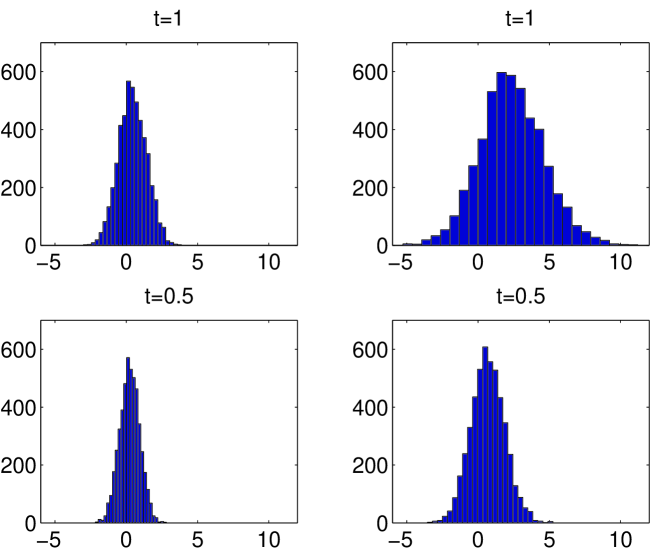
Figure 9: Distribution of $\sum_{i\in S}\ln\lambda_{i}$ (left) and $\eta^{\dagger}\bar{P}(M^{\dagger}M-1)\eta$ (right) contributing to $\tilde{\nu}$ in (5.3).

In the simulations with PSD we also looked at the distribution of the action difference $\Delta$ that appears in (5.3). In Fig.9 we show histograms with the distributions of the two components contributing in (5.3) for the two choices $t=1$ and $t=0.5$. From the measured values of $\Delta$ we extract its mean $m_{s}$ and variance $b_{s}^{2}$. For $t=1$ we get $m_{s}=2.82$ and $b_{s}^{2}=5.90$, for $t=0.5$ we get $m_{s}=0.92$ and $b_{s}^{2}=1.88$ both a factor three smaller than for $t=1$. Inserting these values in (5.6) we obtain acceptance rates in the Gaussian model of 24% for $t=1$ and of 50% for $t=0.5$, in perfect agreement with the acceptance rates directly observed in the simulations.

6 Conclusions

We found that two-dimensional QED can be simulated over a wide range of parameters by a combination of pure gauge update proposals combined with a global Metropolis step including the exactly evaluated determinant for two flavours of Wilson fermions. Employing a coupling for the proposals that differs from the physical one can raise the acceptance rate further and is an example of ultraviolet filtering. This algorithm provides an upper bound for the acceptance rate of a class of stochastic techniques. We studied such methods where we replace the ideal exact determinant ratios by less expensive stochastic estimates whose main cost are inversions of the Dirac operator.

It turned out to be both necessary and possible to find a mixed form of stochastic estimates combined with the exact incorporation of a few critical modes which otherwise spoil the acceptance probability. These modes are given as extremal eigenvalues of the generalized problem defined by the Dirac operators in the present and the newly proposed gaugefield. This was coined PSD algorithm as it is based on the partially stochastic determinant. Gauge fixing proved to be advantageous in this case. If omitted, the update proposals include random relative moves along the gauge orbit which are punished with enhanced rejection. For the physically smaller volumes we found the acceptance rates to be well described by assuming Gaussian distributions for those parts of the total action that enter the Metropolis decision. The rates are then given by error functions of the observed mean and variance. With these insights we plan to investigate similar update schemes for four dimensional QCD, especially at small and intermediate physical volume, and hope to report on this in the future.

Acknowledgements We wish to express our thanks to Burkhard Bunk, Anna Hasenfratz and Rainer Sommer for helpful discussions, and e-mail exchange with Tony Kennedy is acknowledged. All calculations were carried out in Matlab employing its built-in linear algebra tools.

Appendix A Acceptance rate for given spectrum

In this appendix we evaluate the integral

$$F(\lambda_{i})=\prod_{i\in\bar{S}}\left(\int_{0}^{\infty}du_{i}\right)\min\Bigl{[}\exp(-\sum_{i\in\bar{S}}u_{i})\,,\,\prod_{i\in S}\lambda_{i}^{-1}\exp(-\sum_{i\in\bar{S}}\lambda_{i}u_{i})\Bigr{]}.$$ (A.1)

Eigenvalues $0<\lambda_{i}<\infty,i=1\ldots n$ enter here and $S$ is a subset of their indices which may also be empty. The set $\bar{S}$ comprises the remaining indices.

The part, where the first argument of $\min$ is minimal, is given by

$$f(\lambda_{i})=\prod_{i\in\bar{S}}\left(\int_{0}^{\infty}du_{i}\right)\exp(-\sum_{i\in\bar{S}}u_{i})\;\theta\Bigl{[}\sum_{i\in\bar{S}}(1-\lambda_{i})u_{i}-C\Bigr{]}$$ (A.2)

where we abbreviated

$$C=\sum_{i\in S}\ln\lambda_{i}\,.$$ (A.3)

By rescaling integrals the full result is obtained as

$$F(\lambda_{i})=f(\lambda_{i})+(\prod_{i}\lambda_{i}^{-1})f(\lambda_{i}^{-1}),$$ (A.4)

a form which immediately reflects detailed balance in the form

$$\frac{F(\lambda_{i})}{F(\lambda_{i}^{-1})}=\prod_{i}\lambda_{i}^{-1}$$ (A.5)

To evaluate $f$ we use the Fourier representation of the step function

$$\theta(u)=\int_{-i\infty}^{+i\infty}\frac{dz}{2\pi i}\;\frac{\mbox{\rm e}^{zu}}{z+\epsilon},$$ (A.6)

where $u$ is real, $\epsilon$ positive and infinitesimal, and the integration runs along the imaginary axis. Proof: residue theorem. With this inserted into (A.2) the $u$-integrations factorize and can be carried out to yield

$$f(\lambda_{i})=\int_{-i\infty}^{+i\infty}\frac{dz}{2\pi i}\;\frac{\mbox{\rm e}^{-zC}}{z+\epsilon}\;\prod_{j\in\bar{S}}\frac{1}{1-z(1-\lambda_{j})}.$$ (A.7)

Assuming non degenerate $\lambda_{i}$ also this integral is evaluated by the residue theorem. The contour can be closed with negligible contribution in the right or in the left half of the complex plane depending on whether $C$ is positive or negative. Performing the integration for both cases we find

$$f(\lambda_{i})=\left\{\begin{array}[]{rc}\sum_{i\in\bar{S},\lambda_{i}<1}\;\mbox{\rm e}^{\frac{C}{\lambda_{i}-1}}\prod_{j\in\bar{S},j\not=i}\;\frac{\lambda_{i}-1}{\lambda_{i}-\lambda_{j}}&\mbox{ for $C>0$}\\[8.61108pt] 1-\sum_{i\in\bar{S},\lambda_{i}>1}\;\mbox{\rm e}^{\frac{C}{\lambda_{i}-1}}\prod_{j\in\bar{S},j\not=i}\;\frac{\lambda_{i}-1}{\lambda_{i}-\lambda_{j}}&\mbox{ for $C<0$}\end{array}\right.$$ (A.8)

In the special case $C=0$ either closure of the contours is legitimate and the two expressions coincide. The implied identity, which holds for arbitrary non-coinciding $\lambda_{i}$,

$$\sum_{i=1}^{n}\;(\lambda_{i}-1)^{n-1}\prod_{i\not=j=1}^{n}\;\frac{1}{\lambda_{i}-\lambda_{j}}=1$$ (A.9)

can in fact also be verified purely algebraically. To this end we recall the Lagrange polynomials, which are familiar from interpolation and numerical integration,

$$l_{i}(\lambda)=\prod_{j\not=i}\frac{\lambda-\lambda_{j}}{\lambda_{i}-\lambda_{j}}\,,$$ (A.10)

with the property

$$l_{i}(\lambda_{j})=\delta_{ij}\,.$$ (A.11)

We may also introduce a matrix $A$ with elements $a_{ij}$ by expanding

$$l_{i}(\lambda)=\sum_{j}a_{ij}\lambda^{j-1}\,,$$ (A.12)

and in particular its last column is given by

$$a_{in}=\prod_{j\not=i}\frac{1}{\lambda_{i}-\lambda_{j}}\,.$$ (A.13)

The famous Vandermonde matrix $V$ has matrix elements

$$v_{jk}=(\lambda_{k})^{j-1}$$ (A.14)

and in terms of it (A.11) says that $A$ and $V$ are inverse to each other. A particular consequence is the relation

$$\sum_{i}v_{ki}a_{in}=\sum_{i}(\lambda_{i})^{k-1}\prod_{j\not=i}\frac{1}{\lambda_{i}-\lambda_{j}}=\delta_{kn}$$ (A.15)

which also implies (A.9) upon binomial expansion of the numerator.

It now remains to combine the two contributions to $F$ in (A.4). A short calculation leads to the result

$$F=\left\{\begin{array}[]{rc}\prod_{k}\lambda_{k}^{-1}+\sum_{i\in\bar{S},\lambda_{i}<1}(1-1/\lambda_{i})\,\mbox{\rm e}^{\frac{C}{\lambda_{i}-1}}\prod_{j\in\bar{S},j\not=i}\;\frac{\lambda_{i}-1}{\lambda_{i}-\lambda_{j}}&\mbox{ for $C>0$}\\[8.61108pt] 1\quad-\sum_{i\in\bar{S},\lambda_{i}>1}(1-1/\lambda_{i})\,\mbox{\rm e}^{\frac{C}{\lambda_{i}-1}}\prod_{j\in\bar{S},j\not=i}\;\frac{\lambda_{i}-1}{\lambda_{i}-\lambda_{j}}&\mbox{ for $C<0$}\end{array}\right.$$ (A.16)

Note that here the exponentials are both damping and may also be written as

$$\mbox{\rm e}^{\frac{C}{\lambda_{i}-1}}=\prod_{k\in S}(\lambda_{k})^{\frac{1}{\lambda_{i}-1}}\,.$$ (A.17)

For $\bar{S}=\emptyset$ we recognize the deterministic acceptance $\min[1,\prod_{k}\lambda_{k}^{-1}]$. For the fully stochastic case $S=\emptyset$ we may use identity (A.9) and its companion

$$\sum_{i}\;\frac{1}{\lambda_{i}}(\lambda_{i}-1)^{n-1}\prod_{j\not=i}\;\frac{1}{\lambda_{i}-\lambda_{j}}=\prod_{k}\lambda_{k}^{-1}$$ (A.18)

to obtain (4.14).

Appendix B Perturbation theory for generalized eigenvalues

B.1 General expressions

We want to solve the generalized eigenvalue problem

$$H\chi=\lambda H^{\prime}\chi$$ (B.1)

by finding $\lambda$ as stationary values of

$$r(\chi)=\frac{\mu(\chi)}{\mu^{\prime}(\chi)},\;\mu=\chi^{\dagger}H\chi,\;\mu^{\prime}=\chi^{\dagger}H^{\prime}\chi.$$ (B.2)

The operators $H=h^{2},H^{\prime}=h^{\prime 2}$ (all hermitian) possess expansions

$$h = h_{0}+\sum_{k\geq 1}g^{k}h_{k}$$ (B.3)

$$h^{\prime} = h_{0}+\sum_{k\geq 1}g^{k}h^{\prime}_{k}$$ (B.4)

and similarly for $H,H^{\prime}$. We are first interested in the case that $h_{0}$ has a zero mode

$$h_{0}\phi_{0}=0,\;\phi_{0}^{\dagger}\phi_{0}=1,$$ (B.5)

which in perturbation theory is only lifted in second order because we assume

$$\phi_{0}^{\dagger}h_{1}\phi_{0}=\phi_{0}^{\dagger}h^{\prime}_{1}\phi_{0}=0.$$ (B.6)

In this case there is an eigenvector $\phi=\phi_{0}+g\phi_{1}+\mbox{\rm O}(g^{2})$ of $h$,

$$h\phi=\kappa\phi,\quad\kappa=\kappa_{2}g^{2}+\mbox{\rm O}(g^{3}).$$ (B.7)

with

$$h_{0}\phi_{1}+h_{1}\phi_{0}=0$$ (B.8)

and

$$\kappa_{2}=\phi_{0}^{\dagger}(h_{2}-h_{1}(h_{0})^{-1}h_{1})\phi_{0}.$$ (B.9)

We next want to show that to leading order in $g$ the vector $\phi$ is also a stationary point of $r$ with the corresponding generalized eigenvalue $\lambda=r(\phi)(1+\mbox{\rm O}(g))$.

We digress here to a simpler case to show the structure of the argument. Assume we want to know an extremal value of $r(x)=p(x)/q(x)$ close to an already known extremum $p^{\prime}(x_{*})=0$ with a small value of $p(x_{*})/q(x_{*})=\epsilon$. Then we set $x=x_{*}+y$, expand, and find that the extremum of $r$ is at

$$y=\epsilon\,\frac{q^{\prime}(x_{*})}{p^{\prime\prime}(x_{*})}+\mbox{\rm O}(\epsilon^{2})$$ (B.10)

with value $r(x_{*}+y)=\epsilon+\mbox{\rm O}(\epsilon^{2})$ unchanged to leading order of the expansion.

Returning to the real problem we set

$$\chi=\phi+R,\;R^{\dagger}\phi=0.$$ (B.11)

Stationarity of $r$ implies

$$H\chi\,\mu^{\prime}(\chi)=H^{\prime}\chi\,\mu(\chi)$$ (B.12)

It is not too difficult to see that with our Ansatz we get

$$\mu(\chi) = g^{4}\kappa_{2}^{2}+\mbox{\rm O}(g^{6})+|hR|^{2}$$ (B.13)

$$h^{\prime}\chi = g(h^{\prime}_{1}-h_{1})\phi_{0}+\mbox{\rm O}(g^{2})+h^{\prime}R$$ (B.14)

There is a solution to the above equations of the form

$$R=g^{3}\sum_{k\geq 0}g^{k}R_{k}.$$ (B.15)

This implies $\mu(\chi)=\mu(\phi)+\mbox{\rm O}(g^{6})$, $\mu^{\prime}(\chi)=\mu^{\prime}(\phi)+\mbox{\rm O}(g^{4})$ and

$$\lambda = \lambda_{2}g^{2}+\mbox{\rm O}(g^{3})=r(\phi)+\mbox{\rm O}(g^{3})$$ (B.16)

$$\lambda_{2} = \frac{(\kappa_{2})^{2}}{|(h^{\prime}_{1}-h_{1})\phi_{0}|^{2}}$$ (B.17)

Using (B.12) the leading term $R_{0}$ is determined by

$$h_{0}R_{0}=(h^{\prime}_{1}-h_{1})\phi_{0}\,\lambda_{2},\phi_{0}^{\dagger}R_{0}=0$$ (B.18)

with the last condition following from (B.11).

There is another generalized eigenvalue associated with the smallest eigenvalue of $h^{\prime}$. Since the problem has the exact symmetry $H\leftrightarrow H^{\prime},\lambda\leftrightarrow 1/\lambda$ it is clear that the corresponding eigenvalue is $\lambda^{\prime}={\lambda^{\prime}}_{-2}g^{-2}+\mbox{\rm O}(g^{-1})$ with

$$\lambda^{\prime}_{-2}=\frac{|(h^{\prime}_{1}-h_{1})\phi_{0}|^{2}}{(\kappa^{\prime}_{2})^{2}}$$ (B.19)

where $\kappa^{\prime}_{2}$ is as $\kappa_{2}$ in (B.7) but now referring to the lowest eigenvalue of $h^{\prime}$. The respective shift $R^{\prime}$ of the eigenvector $\phi^{\prime}$ has a leading component $(\kappa_{2})^{2}R^{\prime}_{0}=-(\kappa^{\prime}_{2})^{2}R_{0}$.

We now come to the regular generalized eigenvalues associated with the non-nullspace of $h_{0}$, i.e. with zeroth order different from $\phi_{0}$. We expand

$$\chi = \sum_{k\geq 0}g^{k}\chi_{k},\quad h_{0}\chi_{0}\not=0$$ (B.20)

$$\lambda = 1+\sum_{k\geq 1}g^{k}\lambda_{k}$$ (B.21)

and insert this into (B.1) to derive for the first two nontrivial orders

$$(H_{1}-H^{\prime}_{1})\chi_{0} = \lambda_{1}H_{0}\,\chi_{0}$$ (B.22)

$$(H_{1}-H^{\prime}_{1}-\lambda_{1}H_{0})\chi_{1} = -(H_{2}-H^{\prime}_{2}-\lambda_{2}H_{0}-\lambda_{1}H^{\prime}_{1})\chi_{0}\,.$$ (B.23)

Note that the zeroth order is fully degenerate and $\chi_{0}$ is determined only in first order by again a generalized eigenvalue problem. This is similar to ordinary highly degenerate perturbation theory, where a large diagonalization cannot be avoided. Combining the first two orders gives also

$$\lambda_{2}=\frac{\chi_{0}^{\dagger}(H_{2}-H^{\prime}_{2}-\lambda_{1}H^{\prime}_{1})\chi_{0}}{\chi_{0}^{\dagger}H_{0}\chi_{0}}.$$ (B.24)

Two generalized eigenvectors $\chi,\tilde{\chi}$ of (B.1) belonging to different generalized eigenvalues $\lambda\not=\tilde{\lambda}$ are orthogonal in the sense

$$0=\chi^{\dagger}H\tilde{\chi}=\chi^{\dagger}H^{\prime}\tilde{\chi}.$$ (B.25)

In particular, eigenvectors to be constructed now have to be orthogonal to $H$ or $H^{\prime}$ times the two previous ones. Of course, this has to come out automatically, but it is interesting to verify as a consistency check. Using the coincidence with eigenvectors $\phi,\phi^{\prime}$ up to terms of O($g^{3}$), the space, to which $\chi_{0}$ must be orthogonal, may be spanned by the leading orders of $H\phi^{\prime}$ and $H^{\prime}\phi$. A little calculation in ordinary perturbation theory gives

$$H\phi^{\prime}-H^{\prime}\phi = 2g(H_{1}-H^{\prime}_{1})\phi_{0}+\mbox{\rm O}(g^{2})$$ (B.26)

$$H\phi^{\prime}+H^{\prime}\phi = g^{2}(H_{1}-H^{\prime}_{1})H_{0}^{-1}(H_{1}-H^{\prime}_{1})\phi_{0}+\mbox{\rm O}(g^{3}).$$ (B.27)

The orthogonality of solutions $\chi_{0}$ to these directions follows indeed by first projecting both sides of (B.22) on $\phi_{0}^{\dagger}$ and then on $\phi_{0}^{\dagger}(H_{1}-H^{\prime}_{1})H_{0}^{-1}$ and using (B.22) again.

In our real problem we have to deal with the additional spin degree of freedom. Hence there are two zero-modes $\phi_{0\alpha},\alpha=1,2$ of $h_{0}$. These are chosen orthonormal and such that the $2\times 2$ matrix

$$\phi_{0\alpha}^{\dagger}(h_{2}-h_{1}(h_{0})^{-1}h_{1})\phi_{0\beta}=\kappa_{2\alpha}\;\delta_{\alpha\beta}$$ (B.28)

is diagonal. The expansions built upon them generate two generalized eigenvalues which are O($g^{2}$) and two O($g^{-2}$).

B.2 Evaluation for given gaugefields

Here we evaluate $\kappa_{2},\lambda_{2},\lambda^{\prime}_{-2}$ for gaugefields

$$A_{\mu}(x)=\frac{1}{L}\sum_{p}\tilde{A}_{\mu}(p)\exp(ip\cdot x)$$ (B.29)

and an analogous expression for $A^{\prime}$. According to (2.15) we have (for gauge parameter $\xi=0$)

$$\tilde{A}_{\mu}(p)=\sum_{\nu}\epsilon_{\mu\nu}(1-\mbox{\rm e}^{-ip_{\nu}})\tilde{\phi}_{r}(p)$$ (B.30)

with

$$\tilde{\phi}_{r}(p)=\frac{1}{2}(\tilde{\phi}(p)+\tilde{\phi}^{*}(-p))$$ (B.31)

leading to a real $A_{\mu}$.

We consider the expansion of $h=D_{W}\gamma_{5}$ now in the ON-basis of free field states $(1,0)\mbox{\rm e}^{ipx}/L$ and $(0,1)\mbox{\rm e}^{ipx}/L$, i.e. as kernels in momentum space and $2\times 2$ matrices in spin. With $\hat{p}_{\mu}=2\sin(p_{\mu}/2),\stackrel{{\scriptstyle\circ}}{{p}}_{\mu}=\sin(p_{\mu})$ we find

$$h_{0}(p,q) = \left[i\sum_{\mu}\gamma_{\mu}\stackrel{{\scriptstyle\circ}}{{p}}_{\mu}+\hat{p}^{2}/2\right]\gamma_{5}\delta_{pq}$$ (B.32)

$$h_{1}(p,q) = \frac{i}{2L}\sum_{\mu}\left[(\gamma_{\mu}+1)\mbox{\rm e}^{-ip_{\mu}}+(\gamma_{\mu}-1)\mbox{\rm e}^{iq_{\mu}}\right]\gamma_{5}\tilde{A}_{\mu}(p-q)$$ (B.33)

$$h_{2}(p,q) = \frac{1}{4L^{2}}\sum_{\mu}\left[(\gamma_{\mu}+1)\mbox{\rm e}^{-ip_{\mu}}-(\gamma_{\mu}-1)\mbox{\rm e}^{iq_{\mu}}\right]\gamma_{5}\widetilde{A^{2}}_{\mu}(p-q)$$ (B.34)

with $\widetilde{A^{2}}_{\mu}(p-q)=\sum_{r}\tilde{A}_{\mu}(p-r)\tilde{A}_{\mu}(r-q)$. Combinations relevant for (B.28) are

$$h_{2}(0,0) = =\frac{\gamma_{5}}{2L^{2}}\sum_{p}\hat{p}^{2}\,|\tilde{\phi}_{r}(p)|^{2}$$ (B.35)

$$h_{1}(p,0) = \frac{1}{2L}\sum_{\mu}\gamma_{\mu}z_{\mu}(p)\,\tilde{\phi}_{r}(p)$$ (B.36)

with

$$(z_{0},z_{1})=-2i\mbox{\rm e}^{-i(p_{0}+p_{1})/2}\;\Bigl{(}\hat{p}_{0}\cos(p_{1}/2)\,,\,\hat{p}_{1}\cos(p_{0}/2)\Bigr{)}$$ (B.37)

With some calculation we are then able to show

$$h_{1}(0,p)(h_{0}(p,p))^{-1}h_{1}(p,0)=$$ (B.38)

$$\frac{-1}{4L^{2}}\;\left[\hat{p}^{2}(2\hat{p}^{2}-\hat{p}_{0}^{2}\hat{p}_{1}^{2})+i\sum_{\mu}\gamma_{\mu}\stackrel{{\scriptstyle\circ}}{{p}}_{\mu}(4\hat{p}^{2}-2\sum_{\nu}|\epsilon_{\mu\nu}|\,\hat{p}_{\nu}^{4})\right]\;\gamma_{5}\frac{|\tilde{\phi}_{r}(p)|^{2}}{\stackrel{{\scriptstyle\circ}}{{p}}^{2}+\frac{1}{4}(\hat{p}^{2})^{2}}\,.$$

Upon $p$-summation the part odd in $p$ does not contribute and from (B.28) we get

$$\kappa_{22}=-\kappa_{21}=\frac{1}{2L^{2}}\sum_{p}\left[1+\frac{\hat{p}^{2}-\frac{1}{2}\hat{p}_{0}^{2}\hat{p}_{1}^{2}}{\stackrel{{\scriptstyle\circ}}{{p}}^{2}+\frac{1}{4}(\hat{p}^{2})^{2}}\,\right]\hat{p}^{2}\,|\tilde{\phi}_{r}(p)|^{2}$$ (B.39)

Inspecting (2.18) we find on average in the quenched ensemble

$$\langle\;|\tilde{\phi}_{r}(p)|^{2}\;\rangle_{G}=\frac{1}{(\hat{p}^{2})^{2}}.$$ (B.40)

A numerical asymptotic expansion gives

$$\langle\;\kappa_{22}\;\rangle_{G}=\frac{1}{2\pi}\ln L-0.00639327+0.13303\,L^{-2}+\mbox{\rm O}(L^{-4}).$$ (B.41)

Also the mean of the square can be worked out

$$\langle\;(\kappa_{2\alpha})^{2}\;\rangle_{G}=\langle\;\kappa_{2\alpha}\;\rangle_{G}^{2}+0.00773389+0.03112\,L^{-2}+\mbox{\rm O}(L^{-4}).$$ (B.42)

The denominator in (B.17) is given by elements of the $2\times 2$ matrix

$$\sum_{p}(h^{\prime}_{1}(p,0)-h_{1}(p,0))^{\dagger}(h^{\prime}_{1}(p,0)-h_{1}(p,0))=$$ (B.43)

$$\frac{1}{L^{2}}\sum_{p}(\hat{p}^{2}-\frac{1}{2}\hat{p}_{0}^{2}\hat{p}_{1}^{2})\,|\tilde{\phi}^{\prime}_{r}(p)-\tilde{\phi}_{r}(p)|^{2}$$

and produces

$$\langle\;|(h^{\prime}_{1}-h_{1})\phi_{0\alpha}|^{2}\;\rangle_{G}=\frac{1}{\pi}\ln L-0.06162368+0.26607\,L^{-2}+\mbox{\rm O}(L^{-4}).$$ (B.44)

References

- [1] M. Creutz, Quantum Fields On The Computer (Advanced Series on Directions in High Energy Physics — Vol. 11, World Scientific, Singapore, 1992).
- [2] S. Duane, A.D. Kennedy, B.J. Pendleton and D. Roweth, Phys. Lett. B195 (1987) 216.
- [3] S. Gottlieb, W. Liu, D. Toussaint, R.L. Renken and R.L. Sugar, Phys. Rev. D35 (1987) 2531.
- [4] MILC, K. Orginos, D. Toussaint and R.L. Sugar, Phys. Rev. D60 (1999) 054503, hep-lat/9903032.
- [5] A. Hasenfratz and F. Knechtli, Phys. Rev. D64 (2001) 034504, hep-lat/0103029.
- [6] P. Hasenfratz et al., Nucl. Phys. Proc. Suppl. 94 (2001) 627, hep-lat/0010061.
- [7] W. Bietenholz, (2000), hep-lat/0007017.
- [8] MILC, T. DeGrand, Phys. Rev. D63 (2001) 034503, hep-lat/0007046.
- [9] H. Neuberger, Phys. Lett. B417 (1998) 141, hep-lat/9707022.
- [10] ALPHA, A. Bode et al., Phys. Lett. B515 (2001) 49, hep-lat/0105003.
- [11] ALPHA, F. Knechtli et al., (2002), hep-lat/0209025.
- [12] C.B. Lang, (1998), hep-lat/9907017.
- [13] C.R. Gattringer, I. Hip and C.B. Lang, Nucl. Phys. B508 (1997) 329, hep-lat/9707011.
- [14] W. Bardeen, A. Duncan, E. Eichten and H. Thacker, (1997), hep-lat/9705002.
- [15] R. Narayanan, H. Neuberger and P. Vranas, Phys. Lett. B353 (1995) 507, hep-lat/9503013.
- [16] B. Joo, I. Horvath and K.F. Liu, (2001), hep-lat/0112033.
- [17] A. Hasenfratz and F. Knechtli, Comput. Phys. Commun. 148 (2002) 81, hep-lat/0203010.
- [18] M. Hasenbusch, Phys. Rev. D59 (1999) 054505, hep-lat/9807031.
- [19] W.H. Press, B.P. Flannery, S.A. Teukolsky and W.T. Vetterling, Numerical Recipes: The Art of Scientific Computing, 2nd ed. (Cambridge University Press, Cambridge (UK) and New York, 1992).
- [20] P. de Forcrand, Nucl. Phys. Proc. Suppl. 73 (1999) 822, hep-lat/9809145.
- [21] A. Duncan, E. Eichten, R. Roskies and H. Thacker, Phys. Rev. D60 (1999) 054505, hep-lat/9902015.
- [22] A. Hasenfratz and A. Alexandru, (2002), hep-lat/0209071.
- [23] A. Hasenfratz, (2002), hep-lat/0211007.
- [24] R. Frezzotti and K. Jansen, Nucl. Phys. B555 (1999) 432, hep-lat/9808038.
- [25] R. Frezzotti and K. Jansen, Nucl. Phys. B555 (1999) 395, hep-lat/9808011.
- [26] T. Kalkreuter and H. Simma, Comput. Phys. Commun. 93 (1996) 33, hep-lat/9507023.
- [27] G.H. Golub and C.F.V. Loan, Matrix Computations, 3rd ed. (The Johns Hopkins University Press, Baltimore and London, 1996).