SLAC-PUB-9652 UH-511-1018-03 hep-ph/0302014 The self-energy of improved staggered quarks

Abstract

We calculate the fermion self-energy at ${\cal O}(\alpha_{s})$ for the Symanzik improved staggered fermion action used in recent lattice simulations by the MILC collaboration. We demonstrate that the algebraic approach to lattice perturbation theory, suggested by us recently Becher:2002if , is a powerful tool also for improved lattice actions.

I Introduction

In a recent paper Becher:2002if , we have shown that methods familiar from continuum perturbation theory can be used to perform calculations in lattice perturbation theory analytically, except for the numerical evaluation of a small number of lattice “master”-integrals. In short, the calculation proceeds as follows: in a first step, a given loop integral is expanded around the continuum limit using the technique of “asymptotic expansions” for Feynman diagrams, familiar Smirnov:pj from continuum perturbation theory. The expansion splits the original integral into continuum integrals and a set of lattice tadpole integrals. These tadpole integrals are independent of external momenta and masses and are interrelated through a set of algebraic identities. Using these relations, the tadpole integrals can be expressed through a small number of master integrals which are evaluated numerically. In Becher:2002if , we have illustrated this strategy by evaluating the gluon and fermion one-loop self-energies with the standard Wilson action.

We have also asserted that the above techniques are not limited to a particular lattice action or to one loop. While correct in principle, in practice this could turn out to be of little use, given the limitations of available computing power. The goal of the present paper is to investigate if the method proposed in Becher:2002if remains useful for improved lattice actions which are employed in many lattice simulations. In what follows, we perform an analytic one loop calculation with the lattice QCD action used by the MILC collaboration in their recent simulations with three dynamical quarks Bernard:2001av . This is a one-loop Symanzik improved gluon action Luscher:1985zq coupled to improved Kogut-Susskind fermions Kogut:ag ; Lepage:1998vj . This action is accurate up to errors of $O(a^{2}\alpha_{s},a^{4})$. We find that the amount of computer algebra needed for perturbative calculations with such an action is significantly larger than for the simple Wilson action, but they nevertheless turn out to be feasible.

Let us stress an important difference between the purely numerical approach used e.g. in Nobes:2001tf and the algebraic method Becher:2002if which we use in this paper. In order to make use of all algebraic relations, not only the integrals that appear explicitly in the expansion of a given graph, but the entire class of lattice tadpole integrals relevant for a given lattice action needs to be considered. For the present calculation we had to produce a database of roughly 30’000 tadpole integrals that are all expressed in terms of 16 master integrals. This took about a week of CPU time running Maple on a desktop computer. Less than 2000 of those integrals actually occurred in our diagrams. On the other hand, once the database is set up, it can be used for any one-loop calculation involving staggered fermions. In this paper we deal with the simplest example of the quark self-energy and derive the relation between the bare and the pole mass of the quark at order ${\cal O}(\alpha_{s})$. We plan to return to other applications in the near future.

This paper is organized as follows. We start by summarizing the method proposed in Becher:2002if and by pointing out some peculiarities in its application to staggered fermions. The presence of the fermion doublers manifests itself in the appearance of multiple “soft” regions. We then explain our treatment of the improvement terms in the action. In our calculation we expand the improved gluon and fermion propagators in a geometric series around the standard propagators. Since loop integrals are analytic in the improvement terms, this expansion can be performed at the level of the integrand. As a matter of principle, it can be carried to any level of precision desired. Finally, we present the result for the fermion self-energy and conclude.

II Asymptotic expansion around the continuum limit

In this Section we briefly describe the main idea of our approach to lattice perturbation theory Becher:2002if . We are interested in the calculation of quantities in the continuum limit, where the particle masses and external momenta are much smaller than the inverse lattice spacing. It is possible to construct the expansion of a lattice integral around the continuum limit by expanding the integrand, at the expense of introducing an additional (analytic) regulator.

It turns out to be convenient to map the integration region $-\pi<k_{\mu}<\pi$ to infinite volume, by changing the integration variables to

$$\eta_{\mu}=\tan(k_{\mu}/2).$$ (1)

Furthermore, we introduce an intermediate regulator by adding a small quantity $\delta$ to the power of one of the propagators. Keeping the regularization parameter $\delta$ non-zero, we then expand the integrand of the lattice loop integral in the so-called soft and hard regions. The original integral is given by the sum of the soft and hard contributions; in this sum all the terms that are singular in the limit $\delta\to 0$ cancel out. The soft and hard contributions are calculated as follows:

• Soft: assume that all the components of the loop momentum $\eta$ are small, i.e. they comparable to masses $m$ and external momenta $p$ in the problem, $\eta_{i}\sim m,~{}p\ll 1$. Perform the Taylor expansion of the integrand in the small quantities $\eta_{i}$ and $m,p$. The expansion coefficients in this region are standard continuum one loop integrals, regularized analytically. No restriction on the integration region is introduced.

• Hard: assume that all the components of the loop momentum are large, $\eta_{i}\sim 1\gg m,p$ and Taylor expand the integrand in $m,p$. The expansion coefficients are massless lattice tadpole integrals.

As in dimensional regularization, scaleless integrals are set to zero.

While the soft part is given by continuum integrals, the hard part is given by lattice tadpole integrals that do not depend on the process under consideration. Intuitively, this is the case because the hard part arises from the integration region where the loop momentum is comparable to the inverse lattice spacing and therefore much larger than the external momenta. The analytic regularization which we use in what follows, turns out to be very efficient in separating soft and hard momenta modes and allows us to treat them separately. It is important to realize that since the integrals occurring in the hard part are process independent, they can be calculated once and for all for a given lattice action.

In any realistic calculation, many lattice tadpole integrals appear. Fortunately, not all of them are independent. Relations between the integrals are obtained after observing that the integral of a total derivative with respect to one of the variables $\eta_{\mu}$ vanishes (there are no surface terms, thanks to analytic regularization). By explicitly computing the derivative, one finds the algebraic relations (recurrence relations) between the lattice tadpole integrals. It is possible to solve these relations using the Gaussian elimination method and express all the lattice tadpole integrals through a small number of master integrals. For more details we refer to Becher:2002if .

The strategy outlined above does not rely on the specific form of the propagator. In Becher:2002if , we have applied the technique to HQET and to QCD with Wilson fermions and calculated a number of QCD one-loop self-energies. We now show how to use the method to calculate loop integrals for staggered fermions. The staggered fermion action is obtained by reducing the number of components of the fermion field after spin diagonalizing the naive lattice fermion action. In perturbative calculations it is convenient to work with the naive fermion action and perform the staggering only at the end of the calculation.

The fermion doubling inherent in the naive discretization of the fermion action manifests itself in the appearance of multiple soft regions. The sixteen zeros of the inverse propagator of naive fermions,

$$D_{F}=\sum_{\mu}\frac{1}{4}\sin^{2}k_{\mu}=\sum_{\mu}\frac{\eta_{\mu}^{2}}{(1+\eta_{\mu}^{2})^{2}}\,,$$ (2)

in the Brillouin zone give rise to sixteen propagating fermions. Correspondingly loop integrals which involve naive fermion propagators have sixteen soft regions. One of those is the region where all components of the loop momentum $\eta_{i}$ are small. The fifteen additional doubler contributions arise after transforming one or several components of the integration momentum as $\eta_{i}\rightarrow 1/\eta_{i}$ and then expanding the resulting integrand around small $\eta_{i}$. For purely fermionic integrals, the sixteen soft contributions are all equal. In integrals with both boson and fermion propagators, this is not the case: since the boson propagator is far off-shell in all corners of the Brillouin zone, the doubler contributions are different from the genuine soft contribution where all the momenta are small compared to inverse lattice spacing.

The contribution of the hard part is obtained as usual, by expanding the loop integral in external momenta and particle masses. The lattice tadpole integrals that occur in the case at hand are

$$H(\{a_{i}\},n,m)=\prod_{i=1}^{4}\int\frac{d\eta_{i}}{(1+\eta_{i}^{2})^{a_{i}}}\,\frac{1}{D_{B}^{n}}\,\frac{1}{D_{F}^{m+\delta}},$$ (3)

where $D_{B}$ is the standard bosonic propagator expressed through variables $\eta$. Let us stress that the regulator has to be on the fermion propagator in order to regulate both the singularities at $\eta_{\mu}=0$ and $\eta_{\mu}=\infty$. The integration-by-parts and partial fractioning relations for this class of integrals are

$$0 = \bigg{\{}1+2\,a_{i}\,({\bm{a}}_{i}-1)+2\,{\bm{a}}_{i}\,({\bm{a}}_{i}-1)\,n\,{\bm{n}}$$

$$+2\,{\bm{a}}_{i}\,(\,{\bm{a}}_{i}-1)\,(2\,{\bm{a}}_{i}-1)\,(m+\delta)\,{\bm{m}}\bigg{\}}\,H\,,$$

$$0 = \bigg{\{}1-\sum_{i=1}^{d}\,\,{\bm{a}}_{i}\,(1-\,{\bm{a}}_{i})\,{\bm{m}}\bigg{\}}\,H\,,$$ (4)

$$0 = \bigg{\{}1-\sum_{i=1}^{d}(1-\,{\bm{a}}_{i})\,{\bm{n}}\bigg{\}}\,H\,.$$

The operator ${\bm{a}}_{i}$ raises the index $a_{i}$ by one unit, etc. The above relations are sufficient to reduce all integrals $H$ to sixteen master integrals. These can be chosen to be convergent (in the limit $\delta\rightarrow 0$) and are calculated numerically. An efficient method for their evaluation is described in Becher:2002if .

III Improved actions

The lattice artifacts arising in calculations with the simplest discretization of the QCD action turn out to be uncomfortably large, making it difficult to extract physical quantities from simulations with currently accessible lattice spacings. For this reason, many simulations are done with improved actions, which include higher dimensional operators whose coefficients are tuned in such a way as to reduce the cutoff effects arising at finite lattice spacing.

In principle one could apply the procedure for perturbative calculations described above directly to improved actions. The higher derivative terms encountered in these actions complicate the calculation in two ways: (1) The recursion relations for the improved propagators are much more complicated than for the standard case which might lead to problems with finding their solutions and, also, to a larger number of master integrals; (2) The derivative interactions make it necessary to calculate hard integrals with more complicated “tensor” structure, i.e. higher powers of $a_{i}$ in Eq.(3).

In the following we avoid the first complication by expanding the improved propagators around the standard ones. In the soft region, where the momentum flowing through the propagators is small, this expansion is built into our formalism since for small momenta the higher dimensional operators are suppressed by powers of the lattice spacing. For large momentum, on the other hand, these operators are suppressed only numerically, but not parametrically. As we will show this suffices to get the result with reasonable precision.

The disadvantage of expanding the propagators is that very high powers of lattice derivatives appear. For example, the quark gluon coupling of the Symanzik improved staggered quark action involves terms with up to six derivatives. The usual fermion self-energy graph therefore involves 12 powers of the lattice momentum $\widehat{k}_{\mu}$ just from the vertex plus additional powers arising from the expansion of the two propagators. This is why we were forced to compute approximately thirty thousand lattice tadpole integrals to have the full reduction of the integrals that appear in the calculation of the fermion self-energy.

III.1 Improved staggered fermions

The naive discretization of the free fermion action can be improved by adding a third lattice derivative term to the action:

$${\cal L}={\bar{\psi}}_{x}\left[\sum_{\mu}\Delta_{\mu}(1+\frac{b}{6}\Delta^{2}_{\mu})\gamma_{\mu}+m\right]\psi_{x}\,.$$ (5)

The associated fermion propagator

$$D_{F}^{-1}(k)=i\sum_{\mu}\gamma_{\mu}\sin k_{\mu}\,(1+\frac{b}{6}\sin^{2}k_{\mu})+m\,$$ (6)

reproduces, for $b=1$, the free continuum propagator up to terms suppressed as $O(k^{4})$ at low energies. Note that the third order derivative in the above action not only improves the fermion propagator at the origin of the Brillouin zone, but also in all of its corners where some components of the momentum are $\pi$ and doublers appear.

From the above expression it is obvious that the improvement term proportional to $b$ is numerically suppressed over the entire momentum range $-\pi<k<\pi$. For the propagator at the origin

$$\int_{-\pi}^{\pi}\frac{d^{4}k}{(2\pi)^{4}}\,\frac{1}{\sum_{\mu}\sin k_{\mu}^{2}\,(1+b\sin^{2}k_{\mu})^{2}}=\\ 0.6197336-0.1267555\,b+0.0214647\,b^{2}\\ -0.00331\,b^{3}+0.0004803\,b^{4}+\dots{}$$ (7)

the expansion in $b$ is roughly a geometric series with an expansion parameter of $1/6$.

The above action is no longer free of $O(a^{2})$ lattice artifacts, once a gauge field is coupled to the fermion. The standard discretization of the covariant derivative

$$D_{\mu}\psi_{x} =\frac{1}{2}\left[U_{x,\mu}\psi_{n+\hat{\mu}}-U_{x-\hat{\mu},\mu}\psi_{n-\hat{\mu}}\right],$$

$$U_{x,\mu} =e^{-igA_{x,\mu}}$$ (8)

leads to “flavor”-changing interactions, in which a fermion emits gluon with momentum of order $\pi$ and scatters into one of its fifteen partners. The Feynman rule for the quark-gluon coupling of naive fermions

$$i\,g\,(2\pi)^{4}\,\delta^{4}(k_{q}-k_{\bar{q}}+k_{g})\,\sum_{\mu}\gamma_{\mu}\,\cos(\frac{k_{q}^{\mu}+k_{\bar{q}}^{\mu}}{2})$$

shows that the flavor-changing and the flavor-neutral interaction have the same strength. However, in flavor changing interactions momentum of the order of the inverse lattice spacing is transferred to the gluon, taking it far off-shell and thus suppressing the interaction by $O(a^{2})$.

To remove the flavor changing interactions at tree level, Lepage suggested Lepage:1998vj to replace the link field $U_{\mu}(x)$ in the covariant derivative by a “fat” link

$$V^{\prime}_{x,\mu}:=\prod_{\nu\neq\mu}\left.\left(1+\frac{\Delta^{(2)}_{\nu}}{4}\right)\right|_{\rm symm.}U_{x,\mu}-\frac{1}{4}\sum_{\nu\neq\mu}(\nabla_{\rho})^{2}U_{x,\mu}\,.$$ (9)

The derivative interactions in the first term of Eq.(9) have been chosen such that the “flavor”-changing interactions get suppressed, while the second term improves the “flavor”-conserving part. Note that the replacement $U_{\mu}(x)\rightarrow V_{\mu}^{\prime}(x)$ is only done for the first derivative term in Eq. (5).

III.2 Improved gluon propagator

The tree level improved gauge action has the form

$${\cal L}=-\beta\,\sum_{x,\mu>\nu}\{c_{1}P_{\mu\nu}(x)+c_{2}(R_{\mu\nu}+R_{\nu\mu})\},$$ (10)

where $\beta=6/g_{0}^{2}$, $c_{1}=5/3$ and $c_{2}=-1/12$. The plaquette $P_{\mu\nu}$ is the $1\times 1$ Wilson-loop in the $\mu\nu$-plane and the rectangle $R_{\mu\nu}$ is the loop with two steps in the $\mu$ and one in the $\nu$ direction. Parameterizing the link between the lattice site $n$ and $n+\hat{\mu}$ as

$$A_{x,\mu} =\int_{p}\,e^{i(n+\hat{\mu}/2)p}\,A_{\mu}(p)\,,$$

the quadratic part of the gluon Lagrangian in Fourier space is

$${\cal L}_{A^{2}}=A_{\mu}(-p)\left[D_{\mu\nu}+E_{\mu\nu}\right]A_{\nu}(p)$$ (11)

with ($\hat{p}_{\mu}=2\sin p_{\mu}/2$)

$$D_{\mu\nu} ={\widehat{p}^{2}}\,g_{\mu\nu}-\frac{\xi}{1+\xi}\,{\widehat{p}}_{\mu}{\widehat{p}}_{\nu},$$ (12)

$$E_{\mu\nu} =\frac{1}{12}\left[(\mbox{$\sum_{\mu}$}{\widehat{p}}_{\mu}^{4}+{\widehat{p}^{2}}{\widehat{p}}_{\mu}^{2})\,g_{\mu\nu}-({\widehat{p}}_{\mu}^{3}\,{\widehat{p}}_{\nu}+{\widehat{p}}_{\mu}\,{\widehat{p}}_{\nu}^{3})\right]\,.$$

The first term $D_{\mu\nu}$ corresponds to the usual plaquette action obtained by setting $c_{1}=1$, $c_{2}=0$ in Eq.(10). The corresponding propagator is

$$G_{\mu\nu}=D^{-1}_{\mu\nu}=\frac{g_{\mu\nu}}{\widehat{p}^{2}}+\xi\frac{\widehat{p}_{\mu}\,\widehat{p}_{\nu}}{(\widehat{p}^{2})^{2}}\,.$$ (13)

We treat $E$ as a perturbation and expand the improved propagator as

$$G^{\rm Imp}=G-b\;G\cdot E\cdot G+b^{2}\;G\cdot E\cdot G\cdot E\cdot G-\dots$$

The hat variables vary between $-2<{\widehat{p}_{\mu}}<2$. The effect of the improvement is largest in the corners of the Brillouin zone, where the above expansion is a geometric series with expansion parameter $2/3$. For the loop graphs calculated below, the expansion parameter turns out to be around $1/2$. To give an example, consider the expansion of the $\mu\mu$-component of the gluon propagator at the origin. It has the following form:

$$G^{\rm Imp}_{\mu\mu}(x=0)=0.1549334\,(1+\xi/4)-0.0366778\,b\\ +0.014347\,b^{2}-0.0063397\,b^{3}+0.003045\,b^{4}\\ -0.0015511\,b^{5}+0.0008239\,b^{6}+\dots$$ (14)

All given digits are significant. To a good approximation, the expansion is an alternating geometric series with expansion coefficient $1/2$. Assuming that the same pattern is found at higher orders we estimate the remainder of $O(b^{n})$ to be $-1/3$ of the last computed term and estimate

$$G^{\rm Imp}_{\mu\mu}(0)=0.1549\,(1+\xi/4)-0.0266\pm 0.0001\,.$$ (15)

The error has been estimated as half of the remainder. We will encounter the same behavior for the quark self-energy graphs and calculate our final results also in that case with the same prescription.

Let us note that Eq.(14) allows us to compute the so-called “mean link”, a quantity needed to perform tadpole improvement Lepage:1992xa of lattice perturbation theory. At $O(\alpha_{s})$ the mean link in Landau gauge $\xi=-1$ is defined as

$$\langle U_{\mu}(x)/3\rangle=1+\frac{8\pi\alpha_{s}}{3}G^{\rm Imp}_{\mu\mu}(0).$$ (16)

. Using Eq.(14) we easily find:

$$\langle U_{\mu}(x)/3\rangle=1+\alpha_{s}u_{0}=1+\alpha_{s}(\,0.7504\pm 0.001)\,,$$ (17)

in agreement with Ref. Nobes:2001tf .

IV Quark self-energy

The one loop quark self-energy has the form

$$\Sigma(p)=\alpha_{s}\left[ip\,\!\!\!/\Sigma^{(1)}+m\,\Sigma^{(2)}\right]+O(a^{2})\,.$$ (18)

Below, we separately give the contributions of the two graphs in Fig. 1. Since the expressions for the graphs in terms of master integrals are neither short nor particularly illuminating, we have evaluated them numerically. The parameter $b=1$ indicates the order in the expansion of the propagator.

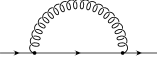
abc

Figure 1: The two graphs contributing to the fermion self-energy.

Soft part

The leading order soft part is obtained by evaluating the continuum diagram in analytic regularization. The reason for that is that all the improvements are subleading and also the fermion doublers decouple in the continuum limit. The doublers contribution is suppressed because the appearance of a doubler requires at least one of the gluon momenta components to be of the order of the lattice spacing.

We therefore get the same result as for Wilson fermions

$$\Sigma^{(1)}_{\rm soft}=(1+\xi)\,\Big{\{}-L_{\delta}+x-\frac{1}{2}+\left(1-x^{2}\right)\,\ln\frac{1+x}{x}\Big{\}}\,,$$

$$\Sigma^{(2)}_{\rm soft}=\left(4+\xi\right)\,\Big{\{}-L_{\delta}-1+(1+x)\,\ln\frac{1+x}{x}\Big{\}}\,.$$

with $x=m^{2}/p^{2}$, $L_{\delta}=1/\delta-\ln(m^{2}/4)$.

Hard part

We now compute the hard part of the tadpole and the sunset diagrams. As it turns out, the tadpole contribution is roughly an order of magnitude larger than that of a sunset; for this reason we have to evaluate more terms in the expansion for the tadpole than for the sunset. We obtain

$$\Sigma^{(1)}_{\rm hard} = 2.6524-1.4214\,b+0.5334\,b^{2}$$

$$-0.2452\,b^{3}+0.1233\,b^{4}$$

$$-0.0655\,b^{5}+(0.3245-0.0345\,b)\,\xi$$

$$= 1.60(1)+0.290\,\xi,$$

$$\Sigma^{(2)}_{\rm hard} = 0.$$

For the hard part of the sunset diagram we find:

$$\Sigma^{(1)}_{\rm hard} = \frac{1+\xi}{3\pi\delta}-0.8327+0.0880\,b-0.0183\,b^{2}$$

$$-(0.6328-0.345\,b)\,\xi,$$

$$\Sigma^{(2)}_{\rm hard} = \frac{4+\xi}{3\pi\delta}-0.9821+0.3279\,b-0.0857\,b^{2}.$$ (20)

Pole mass

It is straightforward to extract the pole mass from the above formulas. The pole mass is defined as the position of the pole of the fermion propagator. It therefore reads:

$$m_{\rm pole} = =m_{\rm bare}\,(1+\alpha_{s}\,\Delta_{1}),$$

$$\Delta_{1} = \Sigma^{(1)}-\Sigma^{(2)}$$ (21)

$$= -\frac{2}{\pi}\ln m+1.60(1)+0.66(1)\,.$$

The first number is the contribution of the tadpole graph, while the second one corresponds to the sunset diagram. Note that the hard and the soft contributions to the pole mass are not gauge invariant separately. This is the consequence of putting the regulator $\delta$ on the fermion propagator, which we are forced to do to properly deal with the doublers. The gauge dependence only cancels in the final result for the pole mass, when the hard and the soft contributions are added together.

The effect of the improvement terms in the lattice action is large. This can be seen by comparing with the result obtained when all the improvements are switched off. In that case the relation between the pole and bare masses changes to

$$m_{\rm pole}^{\rm naive} = =m_{\rm bare}\,(1+\alpha_{s}\,\Delta_{1}^{\rm naive}),$$

$$\Delta_{1}^{\rm naive} = -\frac{2}{\pi}\ln m+4.586\,.$$ (22)

One sees that the renormalization constant in this case is roughly a factor of two larger than for the improved action. The reduction arises because the smearing of the link in Eq. (9) strongly reduces the quark gluon interaction, while the effect of all other improvements is significantly smaller.

Note that the result in Eq.(21) is not “tadpole-improved” Lepage:1992xa . For a tadpole improved action, an additional tree level contribution

$$\Delta^{\rm tad}=-\left(\frac{5}{2}-\frac{b}{4}\right)\,\alpha_{s}\,u_{0}^{(2)}$$ (23)

arises, which tends to cancel the tadpole graph. The quantity $u_{0}^{(2)}$ is the $O(\alpha_{s})$ coefficient of the mean link in Landau gauge, given in Eq.(16) so that

$$\Delta^{\rm tad}=-1.688(2).$$ (24)

Putting everything together, restoring the lattice spacing and combining the numerical errors in quadratures, we derive the following relation between the pole and the bare quark mass in the continuum limit:

$$m_{\rm pole}=m_{\rm bare}\left[1+\alpha_{s}\left(-\frac{2}{\pi}\ln ma+0.572(14)\right)\right].$$ (25)

Our results agree with the findings of Ref. Hein:2001kw . Note that this reference uses the mean field $u_{0}$ defined from the average plaquette, for which $u_{0}^{(2)}\approx 0.7671$ Nobes:2001tf .

V Conclusion

Perturbative calculations with lattice regularization are required to provide a bridge between non-perturbative simulations and the continuum physics. In this paper, we have described an analytic calculation of the fermion self-energy of improved staggered fermions and the Lüscher-Weisz action for gluons. This action has been recently used for non-perturbative lattice simulations by the MILC collaboration.

Our main result, the relation between the pole and the bare lattice quark masses is given in Eq.(25). We observe that the renormalization constant for the improved action is rather modest. This is mainly a consequence of the smearing of the quark-gluon interaction that was introduced to strongly suppress the interaction between the fermions in different corners of the Brillouin zone. Let us stress that in the current calculation the doublers do not contribute in the continuum limit even for the naive action; the strong change in the renormalization constant therefore has not so much to do with their decoupling as with a significant reduction of the quark-gluon interaction interaction over the entire Brillouin zone.

This calculation demonstrates that algebraic techniques for lattice perturbation theory, based on the methods developed for continuum perturbation theory, are quite efficient. With the large database for one-loop lattice tadpole integrals for staggered fermions, which we have produced in the course of this calculations, other one-loop perturbative lattice calculations for improved lattice actions seem to be within reach.

Acknowledgments We are grateful to Q. Mason for providing the Feynman rules for the improved action. We thank C. Anastasiou for letting us use his computer program babis to perform the reduction of to master integrals. This research was supported in part by the DOE grants DE-AC03-76SF00515 and DE-FG03-94ER-40833.

References

- (1) T. Becher and K. Melnikov, Phys. Rev. D 66, 074508 (2002).
- (2) For a review, see V. A. Smirnov, “Applied Asymptotic Expansions In Momenta And Masses,” Berlin, Germany: Springer (2002) 262 p.
- (3) C. W. Bernard et al., Phys. Rev. D 64, 054506 (2001) [arXiv:hep-lat/0104002].
- (4) M. Lüscher and P. Weisz, Phys. Lett. B 158, 250 (1985).
- (5) J. B. Kogut and L. Susskind, Phys. Rev. D 11, 395 (1975).
- (6) G. P. Lepage, Phys. Rev. D 59, 074502 (1999) [arXiv:hep-lat/9809157].
- (7) M. A. Nobes, H. D. Trottier, G. P. Lepage and Q. Mason, Nucl. Phys. Proc. Suppl. 106, 838 (2002) [arXiv:hep-lat/0110051].
- (8) G. P. Lepage and P. B. Mackenzie, Phys. Rev. D 48, 2250 (1993) [arXiv:hep-lat/9209022].
- (9) J. Hein, Q. Mason, G. P. Lepage and H. Trottier, Nucl. Phys. Proc. Suppl. 106, 236 (2002) [arXiv:hep-lat/0110045].
- (10) C. Anastasiou, to be published.