Anisotropic lattice actions for heavy quark

Abstract

The anisotropic lattice fermion actions are investigated with the one-loop perturbative calculations aiming at constructing a formulation for heavy quark with controlled systematic uncertainties. For the heavy-light systems at rest the anisotropic lattice with small temporal lattice spacing $a_{t}$ suppresses the discretization error by a power of $a_{t}m_{Q}$ for a heavy quark of mass $m_{Q}$. We discuss the issue of large discretization errors, which scales as $a_{s}m_{Q}$ with $a_{s}$ the spatial lattice spacing. By performing one-loop calculations of the speed-of-light renormalization for several possible lattice actions in the limit of $a_{t}\rightarrow 0$, we show that one can eliminate the large systematic error on the anisotropic lattice.

I Introduction

In the heavy quark physics, the lattice simulation of Quantum Chromodynamics (QCD) is an indispensable tool to compute hadron masses and matrix elements nonperturbatively without introducing model dependence. One of the most important hadron matrix elements in the $B$ physics is the $B$ meson decay constant $f_{B}$, for which a number of lattice calculations have been performed so far and the systematic uncertainties are under control at the level of 15% accuracy Yamada:2002wh . In future, further precise calculation, say better than 5%, is necessary to constrain the Cabibbo-Kobayashi-Maskawa (CKM) matrix elements more strictly and to search for the signature of new physics.

One of the dominant uncertainties in the lattice simulation of heavy quark is the systematic error associated with the large heavy quark mass, since the lattice cutoff $1/a$ available with current computer power is not much larger than the heavy quark mass $m_{Q}$. A conventional approach to avoid this problem is to restrict ourselves in the region where the systematic error is under control ($m_{Q}\ll 1/a$) and to extrapolate to the $b$ quark mass using the heavy quark scaling law predicted by the heavy quark effective theory (HQET). This is unsatisfactory in order to achieve the 5% accuracy, since the possible error scales as $(am_{Q})^{n}$ ($n$ = 2 for the $O(a)$-improved action) and thus grows very quickly toward heavier quark masses. The extrapolation to the $b$ quark mass could even amplify the systematic uncertainty.

Another method is the HQET-based approach which includes lattice NRQCD Thacker:1990bm ; Lepage:1992tx and the Fermilab method El-Khadra:1997mp . In this method one considers the lattice action for heavy quark as an effective theory valid for large heavy quark masses. The advantage of the HQET-based approach is the absence of the large systematic error which scales as $(am_{Q})^{n}$. The price one has to pay, on the other hand, is the introduction of a number of terms in the action. Their associated coefficients have to be determined by matching the effective theory onto the continuum full theory. The matching is usually carried out using perturbation theory, which limits the accuracy of the lattice calculation.

Besides the HQET-based approach, a possible way to control heavy quark discretization effects is to consider an anisotropic lattice, where the temporal lattice spacing $a_{t}$ is much smaller than the spatial one $a_{s}$ Alford:1996nx ; Klassen:1999fh . Since for a heavy meson (or a heavy baryon) at rest the large energy scale of order $m_{Q}$ appears only in the temporal component in the momentum space, one can expect that the systematic error arises as $(a_{t}m_{Q})^{n}$ and therefore suppressed as far as $a_{t}$ is small enough. The computational cost is not prohibitive if one keeps the spatial lattice spacing relatively large. The problem of the matching of many operators in the effective theory does not appear, as the theory is relativistic.

There is, however, a subtle issue discussed in Harada:2001ei that for a certain choice of the Wilson term in the spatial direction the systematic error may arise in the combination $a_{s}m_{Q}$ rather than the expected $a_{t}m_{Q}$ and the virtue of the anisotropic lattice is spoiled. With an alternative choice the error of order $(a_{s}m_{Q})^{n}$ may be avoided but the unwanted doublers become lighter and disturbs the simulation of physical states. The authors of Aoki:2001ra even denied the advantage of the anisotropic lattice used for heavy quark based on their observation of $a_{s}m_{Q}$-like behavior through radiative corrections. In this paper we discuss this issue further by considering a larger set of $O(a)$-improved lattice fermion actions and by performing one-loop calculations in the limit $a_{t}\rightarrow 0$ where no $a_{t}m_{Q}$ error remains.

The appearance of large systematic errors scaling as $a_{s}m_{Q}$ is naively unexpected for the following reasons. In the $a_{t}\rightarrow 0$ limit the only source of the discretization error is the spatial derivative in the lattice action. In momentum space, therefore, discretization errors scale as $a_{s}p$ with $p$ a typical (spatial) momentum scale in the system, which is of order $\Lambda_{\mathrm{QCD}}$ for the heavy-light mesons or baryons at rest, and the combination $a_{s}m_{Q}$ may not appear as the momentum of order $m_{Q}$ flows only in the temporal direction. This intuitive picture should be correct even after radiative corrections, because the large momentum of order $m_{Q}$ does not flow into the spatial direction in the momentum space, and therefore the discretization error in the spatial lattice derivative cannot accompany the heavy quark mass $m_{Q}$. It becomes clearer if one considers the limit $1/a_{s}\ll m_{Q}\ll 1/a_{t}$, because the spatial momentum integral runs up to $\pi/a_{s}$ and thus cannot pick up the larger scale $m_{Q}$.

Here, in order to understand the reason why the unexpected $a_{s}m_{Q}$-type error may appear in Harada:2001ei ; Aoki:2001ra , let us consider the energy-momentum dispersion relation at the tree level. We consider the $a_{t}\rightarrow 0$ limit, and the spatial lattice spacing is also kept small enough such that we can neglect the error of $O(a_{s}^{2})$ and higher. For the Wilson-type fermions the inverse quark propagator is given as

$$m_{Q}+i\gamma_{0}p_{0}+i\sum_{i}\gamma_{i}p_{i}+\frac{r_{s}}{2\xi}a_{s}\sum_{i}p_{i}^{2}+O(a_{s}^{2}),$$ (1)

where $r_{s}$ denotes the coefficient in front of the spatial Wilson term as defined in (4) in the next section. The term including the anisotropy $\xi=a_{s}/a_{t}$ is maintained even in the $a_{t}\rightarrow 0$ limit, because that term could remain when $r_{s}$ scales as $\xi$. To push up the spatial doubler mass in the cutoff scale, $r_{s}/\xi$ must be kept finite.

The energy-momentum dispersion relation becomes

$$-p_{0}^{2} = \left(m_{Q}+\frac{r_{s}}{2\xi}a_{s}\sum_{i}p_{i}^{2}\right)^{2}+\sum_{i}p_{i}^{2}+O(a_{s}^{2})$$ (2)

$$= m_{Q}^{2}+\left(1+\frac{r_{s}}{\xi}a_{s}m_{Q}\right)\sum_{i}p_{i}^{2}+O(a_{s}^{2}),$$

and thus the error of order $a_{s}m_{Q}$ appears unless $r_{s}/\xi$ vanishes, for which the doublers become light. Since the term $(r_{s}/\xi)a_{s}m_{Q}$ comes from the cross term of the mass and the Wilson terms, the origin of the combination $a_{s}m_{Q}$ is nothing to do with the large momentum flow into the spatial direction. At the tree level we may consider a set of lattice actions in which there is no spatial Wilson term by introducing higher derivative operators to decouple the unwanted doublers. This class of actions does not have the problem of the $O(a_{s}m_{Q})$ error at the tree level and may be used for heavy quark even for $a_{s}m_{Q}>1$. There are higher order terms whose coefficient behaves like $a_{s}m_{Q}$, but we neglect them as their contribution is $O(a_{s}^{2})$ or higher.

The problem is, then, whether the nice property of these actions is maintained even with radiative corrections. In this paper we perform one-loop perturbative calculation for these lattice actions and investigate the mass dependence of the rest mass $M_{1}=E({\bf 0})$ and the kinetic mass $M_{2}=({\partial^{2}E/\partial p_{1}^{2}})^{-1}_{{\bf p}={\bf 0}}$, where $E({\bf p})$ is the energy of heavy quark on-shell. We examine the functional dependence of the speed of light renormalization parameter $\nu$, which is defined such that the relation $M_{1}=M_{2}$ is satisfied. If the one-loop coefficient behaves as $(a_{s}m_{Q})^{n}$, the action suffers from the unwanted heavy quark mass dependent error. Because we are interested only in the $O((a_{s}m_{Q})^{n})$ errors, we carry out the one-loop calculation in the $a_{t}\rightarrow 0$ limit, where $O((a_{t}m_{Q})^{n})$ errors vanish. The fermion actions we consider are the anisotropic SW (Sheikholeslami and Wohlert) action Sheikholeslami:1985ij ; Harada:2001ei and some special cases of the D234 action Alford:1996nx . We find the latter to be useful for applications to heavy quark systems.

This paper is organized as follows. In Section II, we define the anisotropic fermion actions we consider in this paper, and discuss their tree-level properties. The static limit of those actions is considered in Section III. The one-loop calculation is then given in Section IV, whose results are presented in Section V. Section VI is devoted to our conclusions. Some technical details are deferred to the Appendices.

II Anisotropic lattice fermion action

We start with the D234 quark action on the anisotropic lattice Alford:1996nx given by

$$S_{\rm D234}=a_{t}a_{s}^{3}\sum_{x}{\bar{\psi}}(x)Q\psi(x)$$ (3)

$$Q = m_{0}\,+\,\sum_{\mu}\,\nu_{\mu}\gamma_{\mu}\nabla_{\mu}\,(1-b_{\mu}a_{\mu}^{2}\Delta_{\mu})$$ (4)

$$\,-\,{1\over 2}\,a_{t}\,\Bigl{(}\sum_{\mu}r_{\mu}\Delta_{\mu}\,\,+\,\,\,\sum_{\mu<\nu}c_{\rm SW}^{\mu}\sigma_{\mu\nu}F_{\mu\nu}\Bigr{)}\,+\,\sum_{\mu}\nu_{\mu}d_{\mu}a_{\mu}^{3}\Delta_{\mu}^{2}$$

where $a_{0}=a_{t}$ and $a_{i}=a_{s}~{}(i=1,2,3)$ are the temporal and spatial lattice spacings respectively, and

$$(\nu_{0},\nu_{i})=(1,\nu)\,,\,\,\,\,\,\,(b_{0},b_{i})=(b_{t},b_{s})\,,\,\,\,\,\,\,(r_{0},r_{i})=(r_{t},r_{s})\,,$$ (5)

$$(c_{\rm SW}^{0},c_{\rm SW}^{i})=(c_{\rm SW}^{t},c_{\rm SW}^{s})\,,\,\,\,\,\,\,(d_{0},d_{i})=(d_{t},d_{s})\,.\,\,\,$$ (6)

Note that the lattice spacing in front of the Wilson and clover terms is $a_{t}$, not $a_{\mu}$. This notation is similar to the one in Alford:1996nx , but different from those in Klassen:1999fh ; Harada:2001ei . The anisotropy parameter is defined by

$$\xi\equiv a_{s}/a_{t}.$$ (7)

The lattice covariant derivatives $\nabla_{\mu}$, $\Delta_{\mu}$, $\nabla_{\mu}\Delta_{\mu}$ and $\Delta_{\mu}^{2}$ represent $D_{\mu}$, $D_{\mu}^{2}$, $D_{\mu}^{3}$ and $D_{\mu}^{4}$, respectively, in the continuum theory, and their detailed definitions are given in Appendix A.

In this paper we always set

$$r_{t}=1\,,\ \ \ b_{t}=d_{t}=0\,.$$ (8)

Thus, the operator $Q$ is nothing but the Wilson-Dirac operator as far as the temporal derivatives are concerned. With this condition, the energy-momentum relation for the fermion has a physical solution only, and the unphysical temporal doublers do not appear Alford:1996nx .

Solving $Q(p)Q(p)^{\dagger}=0$ in the momentum space and then setting $p_{0}=iE$, we obtain the energy-momentum relation for the D234 action as

$$4\sinh^{2}({a_{t}E\over 2})~{}=~{}\frac{\nu^{2}a_{t}^{2}\sum_{i}\bar{p_{i}}^{2}(1+b_{s}a_{i}^{2}\hat{p_{i}}^{2})^{2}+\mu({\bf p})^{2}}{1+\mu({\bf p})}\,,$$ (9)

where

$$\mu({\bf p}) = a_{t}m_{0}+{1\over 2}r_{s}a_{t}^{2}\sum_{i}\hat{p}_{i}^{2}+\nu d_{s}a_{t}\sum_{i}a_{i}^{3}\hat{p}_{i}^{4}~{},$$ (10)

and ${\bar{p}}_{\mu}$ and $\hat{p}_{\mu}$ are defined in Appendix A.

From (9), we obtain the tree-level rest mass $M_{1}=E({\bf 0})$ and kinetic mass $M_{2}=({\partial^{2}E/\partial p_{1}^{2}})^{-1}_{{\bf p}={\bf 0}}$ as

$$a_{t}M_{1} = \log(1+a_{t}m_{0})\,,$$ (11)

$$\frac{1}{a_{t}M_{2}} = \frac{2\nu^{2}}{a_{t}m_{0}(2+a_{t}m_{0})}+\frac{r_{s}}{1+a_{t}m_{0}}\,.$$ (12)

On the anisotropic lattice with $a_{t}m_{0}\ll 1$, the tree-level mass ratio $M_{1}/M_{2}$ can be expanded in terms of $a_{t}m_{0}$ as

$$M_{1}/M_{2}=1+(r_{s}-1)\,a_{t}m_{0}+O((a_{t}m_{0})^{2})\,,$$ (13)

where we set $\nu=1$. The deviation of $M_{1}/M_{2}$ from unity is a lattice discretization error arising from the fermion mass. Unless $r_{s}\propto\xi$, such an error is a function of $a_{t}m_{0}$ alone, which is small on the anisotropic lattice with $a_{t}m_{0}\ll 1$ Harada:2001ei . When $r_{s}\propto\xi$, a discretization error of order $a_{s}m_{0}=\xi a_{t}m_{0}$ arises, which is still large on the anisotropic lattice.

From (9), we can also calculate the “spatial-doubler” mass $E^{d}$, i.e. the energy at the edge of the Brillouin zone ($p_{i}=\pi/a_{s}$):

$$a_{t}E^{d} = \log\biggl{[}1+a_{t}m_{0}+\frac{2r_{s}}{\xi^{2}}n_{d}+\frac{16\nu d_{s}}{\xi}n_{d}\biggr{]}$$ (14)

$$\equiv \log[1+a_{t}m_{0}^{d}]\,,$$ (15)

where $n_{d}$ (= 1, 2, 3) is the number of spatial direction with $p_{i}=\pi/a_{s}$, and the bare spatial-doubler mass $m_{0}^{d}$ is given by

$$a_{s}m_{0}^{d}=a_{s}m_{0}+\frac{2r_{s}}{\xi}n_{d}+16\nu d_{s}n_{d}\,$$ (16)

in units of the spatial lattice spacing $a_{s}$. We note that one has to take $r_{s}\propto\xi$ or $d_{s}>0$ in order to decouple the spatial-doubler with the energy $E^{d}$ from the physical state for large values of $\xi$.

It is interesting to consider the energy-momentum relation in the Hamiltonian limit $a_{t}\rightarrow 0$ ($\xi\rightarrow\infty$), where $a_{t}m_{0}$ errors vanish. In this limit the left-hand side of (9) is replaced by $a_{t}^{2}E^{2}$, and the energy-momentum relation is simplified to

$$E^{2}(a_{t}\rightarrow 0) \!=\! \nu^{2}\sum_{i}\bar{p_{i}}^{2}(1+b_{s}a_{i}^{2}\hat{p_{i}}^{2})^{2}+\frac{\mu({\bf p})^{2}}{a_{t}^{2}}$$ (17)

$$\!=\! m_{0}^{2}+\nu^{2}{\bf p}^{2}+\biggl{(}-\frac{\nu^{2}}{3}+2\nu^{2}b_{s}+2a_{s}m_{0}\nu d_{s}\biggr{)}a_{s}^{2}\sum_{i}p_{i}^{4}+O(a^{4}p^{6})\,.$$ (18)

From a small ${\bf p}$ expansion we obtain a non-relativistic expression of $E(a_{t}\rightarrow 0)$:

$$E(a_{t}\rightarrow 0)=m_{0}+\frac{\nu^{2}}{2m_{0}}{\bf p}^{2}-\frac{\nu^{4}}{8m_{0}^{3}}({\bf p}^{2})^{2}+\frac{1}{2m_{0}}\biggl{(}-\frac{\nu^{2}}{3}+2\nu^{2}b_{s}+2a_{s}m_{0}\nu d_{s}\biggr{)}a_{s}^{2}\sum_{i}p_{i}^{4}+O(a^{5}p^{6})\,.$$ (19)

Taking the static limit $m_{0}\rightarrow\infty$ subsequently, one obtains

$$E(a_{t}\rightarrow 0)~{}\stackrel{{\scriptstyle m_{0}\rightarrow\infty}}{{\longrightarrow}}~{}m_{0}+\nu d_{s}a_{s}^{3}\sum_{i}p_{i}^{4}+O(a^{5}p^{6})\,.$$ (20)

Note that the $\sum_{i}p_{i}^{4}$ term survives even in the static limit. This will be discussed later.

We are now ready to define our anisotropic actions more explicitly. We study two actions: one is the SW action Sheikholeslami:1985ij ; Harada:2001ei , and the other is a variant of the D234 action Alford:1996nx , which we call the sD34 action. We give these actions and discuss their tree-level properties in the following.

II.1 SW action

The Sheikholeslami-Wohlert (SW) action Sheikholeslami:1985ij ; Harada:2001ei is defined by

$$\nu=r_{s}=c_{\rm SW}^{\mu}=1\,,\ \ b_{s}=d_{s}=0\,.$$ (21)

An $O(a_{t})$ error arising from the Wilson terms is removed by $c_{\rm SW}^{\mu}=1$. Since the Wilson terms are $O(a_{t})$, this action goes over to the “naive” quark action in the $a_{t}\rightarrow 0$ ($\xi\rightarrow\infty$) limit. The energy splitting between the physical state and spatial-doublers $E^{d}-E$ vanishes in this limit, as one can explicitly find from (16). The energy-momentum relation for the SW action is shown in Figure 1. The energy at the edge of the Brillouin zone decreases as $\xi$ increases, which shows the reappearance of the spatial-doubler.

Since $r_{s}=1$, the tree-level mass ratio $M_{1}/M_{2}$ (Eq. (13)) contains no $O((a_{s}m_{0})^{n})$ error: $M_{1}/M_{2}=1+O((a_{t}m_{0})^{2})~{}\stackrel{{\scriptstyle a_{t}\rightarrow 0}}{{\longrightarrow}}~{}1$. The anisotropic SW action has been applied to the simulation of charmonium Umeda:2000ym and the charmed hadrons Matsufuru:2001cp ; Harada:2002rf on $\xi\simeq 4$ anisotropic lattices.

II.2 sD34 action

We define the sD34 action as

$$r_{s}=c_{\rm SW}^{s}=0\,,\ \ b_{s}>0\,,\ \ d_{s}>0.$$ (22)

Although the spatial Wilson term is absent ($r_{s}=0$), this action is doubler-free because $d_{s}>0$. The energy splitting $E^{d}-E$ remains even in the $a_{t}\rightarrow 0$ limit as far as $d_{s}$ is a constant independent of $\xi$. Setting $d_{s}=1/8$ for this action gives the same spatial-doubler mass $m_{0}^{d}$ as for the $\xi=1$ SW action when $\nu=1$. The name “sD34” is a reminder that the spatial $\gamma_{i}D_{i}^{3}$ and $D_{i}^{4}$ terms survive in the $a_{t}\rightarrow 0$ limit. The sD34 action is similar to the one proposed in Hamber:1983qa ; Eguchi:1983xr , except that those papers consider the case of the isotropic lattice $\xi=1$. Since the sD34 action has the next-nearest neighbor interactions such as ${\bar{\psi}}\nabla_{\mu}\Delta_{\mu}\psi$ and ${\bar{\psi}}\Delta_{\mu}^{2}\psi$, this action is more costly to simulate than the SW action which consists of the nearest neighbor interactions only.

The sD34 action does not generate $O(a_{s})$ discretization errors because of $r_{s}=c_{\rm SW}^{s}=0$. In order to remove an $O(a_{t})$ error arising from the temporal Wilson term with $r_{t}=1$, we take

$$\nu=1+\frac{1}{2}r_{t}a_{t}m_{0}\,,\ \ c_{\rm SW}^{t}=\frac{1}{2}\,.$$ (23)

This condition is obtained by performing a field redefinition $\psi_{c}=\Omega_{c}\psi$, ${\bar{\psi}}_{c}={\bar{\psi}}{\bar{\Omega}}_{c}$, ${\bar{\Omega}}_{c}=\Omega_{c}=1-{1\over 4}r_{t}a_{t}(D\!\!\!\!/\,_{0}-m_{c})$ to the continuum quark action ${\bar{\psi}}_{c}(x)(D\!\!\!\!/\,+m_{c})\psi_{c}(x)$ Alford:1996nx . Since $r_{s}=0$ the tree-level mass ratio $M_{1}/M_{2}$ again contains no $O((a_{s}m_{0})^{n})$ errors: $M_{1}/M_{2}=1+O((a_{t}m_{0})^{2})~{}\stackrel{{\scriptstyle a_{t}\rightarrow 0}}{{\longrightarrow}}~{}1$.

In the rest of paper we consider the following three choices of $b_{s}$ and $d_{s}$ parameters:

$$b_{s}=\frac{1}{6}\,,\ \ \ \ d_{s}=\frac{1}{8}\, : {\rm~{}sD34~{}~{}~{}~{}~{}},$$ (24)

$$b_{s}=\frac{1}{8}\,,\ \ \ \ d_{s}=\frac{1}{8}\, : {\rm~{}sD34(v)~{}},$$ (25)

$$b_{s}=\frac{1}{2}\,,\ \ \ \ d_{s}=\frac{1}{4}\, : {\rm~{}sD34(p)~{}}.$$ (26)

The first choice sD34, where $b_{s}=1/6$, eliminates an $O(a_{s}^{2})$ error arising from the $\gamma_{i}\nabla_{i}$ term: $\gamma_{i}\nabla_{i}(1-\frac{1}{6}a_{s}^{2}\Delta_{i})=\gamma_{i}D_{i}+O(a_{s}^{4})$. The second choice sD34(v), where $b_{s}=1/8$, eliminates an $O(a_{s}^{2})$ error in the one-gluon vertex (98): $V_{1,i}^{a}(q,q^{\prime},k)=-igt^{a}\gamma_{i}+O(a_{s}^{3})$. The difference between the one-loop results for sD34 and for sD34(v) is numerically small as shown in the next section. With the third choice sD34(p), the hopping terms in the action are proportional to the projection matrix $1\pm\gamma_{\mu}$: using the Wilson’s projection operator $w_{\mu}~{}\equiv~{}a_{\mu}\gamma_{\mu}\nabla_{\mu}-\frac{1}{2}a_{\mu}^{2}\Delta_{\mu}$, the space-component of the action is given by $w_{i}+{\textstyle{1\over 2}}w_{i}^{2}$ ($i=1,2,3$). Therefore the third choice can reduce simulation costs compared to the other two choices Alford:1996nx . At the tree level the sD34 action (24) is $O(a_{s}^{2})$-improved, while others contain some $O(a_{s}^{2})$ errors. Within the current set of operators (4), therefore, the best available choice to suppress discretization effects is the sD34 action.

The energy-momentum relations for the sD34 and sD34(p) actions are shown in Figures 2 and 3 respectively. For both choices the energy at the edge of the Brillouin zone increases as $\xi$ increases, in contrast to the case of the SW action. In small $a_{s}{\bf p}$ region, the energy-momentum relation for the sD34 action is quite close to the continuum one because it has no $O(a_{s}^{2}{\bf p}^{2})$ errors. Moreover, in large $a_{s}{\bf p}$ region near the edge of the Brillouin zone, it is close to the continuum one too, for large values of $\xi$.

To summarize, both the SW action and the sD34 action do not generate the $O((a_{s}m_{Q})^{n})$ ($n=1,2,\cdots$) errors at the tree level in the mass ratio $M_{1}/M_{2}$. While the SW action suffers from the spatial doubler for large values of $\xi$, the sD34 action is doubler-free for any value of $\xi$. Both actions can be used for simulations of the charm quark, if $\xi\simeq 2-4$ and $a_{t}m_{c}\ll 1$. But simulations of the bottom quark keeping $a_{t}m_{b}\ll 1$ require $\xi\simeq 5-10$, for which the anisotropic SW action may be contaminated by the spatial doublers.

Besides the above actions, two other anisotropic actions have been proposed and applied to heavy quark systems: one is the action with $r_{t}=1$ and $r_{s}=\xi$ Klassen:1999fh ; Chen:2001ej ; Okamoto:2001jb ; Mei:2002ip , and the other is that with $r_{t}=r_{s}=\xi$ Groote:2000jd ; Collins:2001pe ; Shigemitsu:2002wh . However, these actions has the spatial Wilson term scaling as $r_{s}=\xi$ and therefore generate the $O((a_{s}m_{0})^{n})$ errors in the mass ratio $M_{1}/M_{2}$ even at the tree level when $\nu=1$, as discussed before and in Harada:2001ei . For this reason, we do not consider these actions further in this paper.

III Static limit $m_{Q}\rightarrow\infty$ and the Hamiltonian limit $a_{t}\rightarrow 0$

In this section we discuss the static limit $m_{Q}\rightarrow\infty$ of the anisotropic fermion actions. At finite $a_{t}$, the action always approaches to the usual static action in the limit of $a_{t}m_{Q}\rightarrow\infty$. This is shown, e.g. by rescaling the fermion field in (3) as

$$\psi(x)=\frac{e^{-a_{t}M_{1}\cdot t}}{\sqrt{a_{t}m_{0}}}h(x)\,,$$ (27)

and then taking $a_{t}m_{0}\rightarrow\infty$.

On the other hand, the action in the limit of $m_{Q}\rightarrow\infty$ while keeping the condition $a_{t}m_{Q}\ll 1$ can be different. In the $a_{t}\rightarrow 0$ limit, the lattice Dirac operator (4) becomes

$$Q(a_{t}\rightarrow 0)=m_{0}\,+\,\gamma_{0}D_{0}\,+\,\nu\sum_{i}\,\gamma_{i}\nabla_{i}\,(1-b_{s}a_{i}^{2}\Delta_{i})\,+\,\nu d_{s}a_{s}^{3}\sum_{i}\Delta_{i}^{2},$$ (28)

unless $r_{s}\propto\xi$. Taking subsequently the static limit, the fermion field splits as usual into large and small components in the Dirac representation of the Dirac matrix, and the off-diagonal terms drop out, the action becomes

$$Q(a_{t}\rightarrow 0) ~{}\stackrel{{\scriptstyle m_{Q}\rightarrow\infty}}{{\longrightarrow}}~{} m_{0}\,+\,\gamma_{0}D_{0}\,+\,\nu d_{s}a_{s}^{3}\sum_{i}\Delta_{i}^{2}\,.$$ (29)

We note that the $a_{s}^{3}\Delta_{i}^{2}$ term, proportional to $\nu d_{s}$, remains in the static limit. The SW action with $d_{s}=0$ approaches the usual static action, but the sD34 action with $d_{s}>0$ does not. This observation is consistent with the static energy evaluated in the $a_{t}\rightarrow 0$ limit (20). Formally the static limit (29) can be derived by applying the Foldy-Wouthuysen-Tani transformation

$$\psi(x)\;\longrightarrow\;\exp\left[-\frac{\nu}{2m_{0}}\sum_{i}\,\gamma_{i}\nabla_{i}\,(1-b_{s}a_{i}^{2}\Delta_{i})\right]\,\psi(x)$$ (30)

to (28) and then taking $m_{0}\rightarrow\infty$.

Results of the one-loop calculation at $a_{t}=0$ in the next section should be consistent with the form (29) in the $m_{Q}\rightarrow\infty$ limit. Suppose that the static action is renormalized as

$$(m_{0}+\delta_{m})\,+\,\gamma_{0}D_{0}\,-\,{1\over 2}\,\delta_{r}a_{s}\,\sum_{i}\Delta_{i}\,+\,(\nu d_{s}+\delta_{d})a_{s}^{3}\sum_{i}\Delta_{i}^{2}\,,$$ (31)

then the mass shift $\delta_{m}$, the kinetic term renormalization $\delta_{r}$, and $\delta_{d}$ do not depend on $m_{0}$, but may depend on $\nu d_{s}$ because the static propagator and vertices contain $\nu d_{s}$ through (29).

IV One-loop calculation in the Hamiltonian limit

In this section we present the one-loop calculations for the anisotropic actions defined in Section II. We calculate one-loop corrections to the rest mass and the kinetic mass renormalization factors in the Hamiltonian limit $a_{t}\rightarrow 0$. From the latter we obtain the one-loop correction to the $\nu$ parameter.

IV.1 Formalism

In the one-loop calculation we basically follow the notation of Mertens:1997wx and add some extensions to the case of the anisotropic lattice.

We write the inverse free quark propagator as

$$a_{t}G_{0}^{-1}(p)=ia_{t}K\!\!\!\!/\,(p)+a_{t}L(p),$$ (32)

and the self energy as

$$a_{t}\Sigma(p) = i\sum_{\mu}\gamma_{\mu}A_{\mu}(p)\sin(a_{\mu}p_{\mu})+C(p)$$ (33)

$$\equiv i\sum_{\mu}\gamma_{\mu}B_{\mu}(p)+C(p)\,,$$

where $p$ is the external momentum. The inverse full quark propagator is then given by

$$G^{-1}(p)=G_{0}^{-1}(p)-\Sigma(p).$$ (34)

Solving $G^{-1}(G^{-1})^{\dagger}=0$ with $p_{0}=iE$, we obtain the all-orders dispersion relation

$$1+\mu({\bf p})-\cosh(a_{t}E)-C=\sqrt{(1-A_{0})^{2}\sinh^{2}(a_{t}E)-{\textstyle\sum_{i}(a_{t}K_{i}-A_{i}\sin(a_{s}p_{i}))^{2}}}\,,$$ (35)

where $\mu({\bf p})$ is given in (10).

Setting ${\bf p}={\bf 0}$ in (35), we obtain the rest mass $M_{1}=E({\bf 0})$ as

$$e^{a_{t}M_{1}} = 1+a_{t}m_{0}+A_{0}(iM_{1},{\bf 0})\sinh(a_{t}M_{1})-C(iM_{1},{\bf 0})$$ (36)

$$= 1+a_{t}m_{0}-iB_{0}(iM_{1},{\bf 0})-C(iM_{1},{\bf 0}).$$

In order to have massless quarks remain massless at the quantum level, we need a mass subtraction. Defining the critical bare mass $a_{t}m_{0c}\equiv C(0,{\bf 0})$, we can write

$$e^{a_{t}M_{1}}=1+a_{t}M_{0}-iB_{0}(iM_{1},{\bf 0})-C_{\rm sub}(iM_{1},{\bf 0}),$$ (37)

where $M_{0}=m_{0}-m_{0c}$ and $C_{\rm sub}(iM_{1},{\bf 0})=C(iM_{1},{\bf 0})-a_{t}m_{0c}$. When $M_{0}=0$, the rest mass $M_{1}$ vanishes by construction. Usually the mass subtraction is done nonperturbatively in the numerical simulation by defining the critical hopping parameter.

In perturbation theory the rest mass is expanded as

$$M_{1}=\sum_{l=0}^{\infty}g^{2l}M_{1}^{[l]},$$ (38)

in which the tree-level rest mass is

$$a_{s}M_{1}^{[0]}=\xi\log(1+a_{t}M_{0})~{}\stackrel{{\scriptstyle a_{t}\rightarrow 0}}{{\longrightarrow}}~{}a_{s}M_{0},$$ (39)

while the one-loop coefficient is given by

$$a_{s}M_{1}^{[1]} = \left(-i\xi B_{0}^{[1]}(iM_{1},{\bf 0})-\xi C^{[1]}_{\rm sub}(iM_{1},{\bf 0})\right)e^{-a_{t}M_{1}^{[0]}}$$ (40)

$$~{}\stackrel{{\scriptstyle a_{t}\rightarrow 0}}{{\longrightarrow}}~{} -i\xi B_{0}^{[1]}(iM_{1},{\bf 0})-\xi C^{[1]}_{\rm sub}(iM_{1},{\bf 0}).$$

Note that $M_{1}$ is now normalized by the spatial lattice spacing $a_{s}$. Before the subtraction the one-loop coefficient is given by

$$a_{s}M_{1,\rm nosub}^{[1]}~{}\stackrel{{\scriptstyle a_{t}\rightarrow 0}}{{\longrightarrow}}~{}-i\xi B_{0}^{[1]}(iM_{1},{\bf 0})-\xi C^{[1]}(iM_{1},{\bf 0})\,.$$ (41)

Differentiating (35) in terms of $p_{1}$ twice and then setting ${\bf p}={\bf 0}$, we obtain the kinetic mass $M_{2}=(\partial^{2}E/\partial p_{1}^{2})^{-1}_{{\bf p}={\bf 0}}$ as

$$\frac{e^{a_{t}M_{1}}-A_{0}(iM_{1},{\bf 0})\cosh(a_{t}M_{1})}{\xi^{2}a_{t}M_{2}}=\frac{r_{s}}{\xi^{2}}+D({\bf 0})+\frac{[\nu/\xi-A_{1}(iM_{1},{\bf 0})]^{2}}{[1-A_{0}(iM_{1},{\bf 0})]\sinh(a_{t}M_{1})},$$ (42)

where

$$D({\bf 0}) = \frac{d^{2}~{}}{d(a_{s}p_{1})^{2}}\left[A_{0}(iE({\bf p}),{\bf p})\sinh(a_{t}M_{1})-C(iE({\bf p}),{\bf p})\right]_{{\bf p}={\bf 0}}$$ (43)

$$= D_{1s}({\bf 0})+\frac{i}{a_{s}M_{2}}D_{1t}({\bf 0})+\frac{i}{a_{s}M_{2}}\cdot\frac{B_{0}(iM_{1},{\bf 0})}{\xi\tanh(a_{t}M_{1})}$$

with

$$D_{1s}({\bf 0}) = \frac{\partial^{2}~{}}{\partial(a_{s}p_{1})^{2}}\left[\frac{1}{i}B_{0}-C\right]_{p=(iM_{1},{\bf 0})},$$ (44)

$$iD_{1t}({\bf 0}) = \frac{\partial~{}}{\partial(a_{s}p_{0})}\left[B_{0}-iC\right]_{p=(iM_{1},{\bf 0})}.$$ (45)

The kinetic mass is expanded as

$$M_{2}=\sum_{l=0}^{\infty}g^{2l}M_{2}^{[l]},$$ (46)

and the tree level relation becomes

$$\frac{e^{a_{t}M_{1}^{[0]}}}{a_{t}m_{2}}=r_{s}+\frac{\nu^{2}}{\sinh(a_{t}M_{1}^{[0]})}$$ (47)

where $M_{2}^{[0]}=m_{2}(M_{1}^{[0]})$.

From (42) and (47), we can obtain the kinetic mass renormalization factor defined by

$$Z_{M_{2}}\equiv\frac{M_{2}}{m_{2}(M_{1})}=1+\sum_{l=1}^{\infty}g^{2l}Z_{M_{2}}^{[l]}\,.$$ (48)

Here the argument of $m_{2}$ is the all-orders rest mass $M_{1}$. The one-loop coefficient is given by

$$Z_{M_{2}}^{[1]}~{}=~{} \frac{2\nu\xi A_{1}^{[1]}(iM_{1},{\bf 0})-\nu^{2}A_{0}^{[1]}(iM_{1},{\bf 0})-D^{[1]}({\bf 0})\xi^{2}\sinh(a_{t}M_{1})}{\nu^{2}+r_{s}\sinh(a_{t}M_{1})}$$ (49)

$$-A_{0}^{[1]}(iM_{1},{\bf 0})\cosh(a_{t}M_{1})e^{-a_{t}M_{1}}.$$

In the $a_{t}\rightarrow 0$ limit, the tree-level kinetic mass goes to

$$\frac{1}{m_{2}}~{}\stackrel{{\scriptstyle a_{t}\rightarrow 0}}{{\longrightarrow}}~{}\frac{\nu^{2}}{M_{1}}+R_{s}a_{s}\,,$$ (50)

where we defined $R_{s}\equiv r_{s}/\xi$, and hence $Z_{M_{2}}$ goes to

$$Z_{M_{2}}~{}\stackrel{{\scriptstyle a_{t}\rightarrow 0}}{{\longrightarrow}}~{}\frac{M_{2}}{M_{1}}\nu^{2}+R_{s}a_{s}M_{2}\,.$$ (51)

Therefore, in this limit, the renormalized $\nu$ parameter and $R_{s}$ which give $M_{1}=M_{2}$ can be determined from $Z_{M_{2}}$:

$$Z_{M_{2}} ~{}\stackrel{{\scriptstyle a_{t}\rightarrow 0}}{{\longrightarrow}}~{} \nu^{2}+R_{s}a_{s}M_{1}$$ (52)

$$= 1+(2\nu^{[1]}+R_{s}^{[1]}a_{s}M_{1}^{[0]})g^{2}+O(g^{4})$$

with the one-loop coefficient

$$Z_{M_{2}}^{[1]}=2\nu^{[1]}+R_{s}^{[1]}a_{s}M_{1}^{[0]}\,.$$ (53)

Here we used $R_{s}^{[0]}~{}\stackrel{{\scriptstyle a_{t}\rightarrow 0}}{{\longrightarrow}}~{}0$.

On the other hand, from (49) we obtain in this limit

$$Z_{M_{2}}^{[1]}~{}\stackrel{{\scriptstyle a_{t}\rightarrow 0}}{{\longrightarrow}}~{}\frac{2}{\nu}\,\xi A_{1}^{[1]}(iM_{1},{\bf 0})-\frac{2}{i}\,\frac{\xi B_{0}^{[1]}(iM_{1},{\bf 0})}{a_{s}M_{1}}-a_{s}m_{2}\xi D^{[1]}({\bf 0})\,,$$ (54)

where $A_{1}^{[1]}(iM_{1},{\bf 0})=\frac{\partial~{}B_{1}^{[1]}}{\partial(a_{s}p_{1})}|_{p=(iM_{1},{\bf 0})}$.

IV.2 One-loop diagrams

Here we compute one-loop contributions relevant to the rest mass and the kinetic mass renormalization. At the one-loop level, the self-energy is written as

$$\Sigma^{[1]}(p)=\Sigma^{\rm reg}(p)+\Sigma^{\rm tad}(p)+\Sigma^{\rm T.I.}(p),$$ (55)

where the contribution from the regular graph Fig. 4(a) is denoted by $\Sigma^{\rm reg}(p)$, while the tadpole graph Fig. 4(b) gives $\Sigma^{\rm tad}$. In order to remove the bulk of $\Sigma^{\rm tad}$, we apply the tadpole improvement Lepage:1993xa , which amounts to $\Sigma^{\rm T.I.}$. Feynman rules relevant to our calculations are summarized in Appendix A. We use the anisotropic Wilson gluon action given by

$$S_{g}=\frac{6}{g^{2}}\left[\xi\sum_{x,i}(1-P_{0i}(x))+\frac{1}{\xi}\sum_{x,i>j}(1-P_{ij}(x))\right]\,,$$ (56)

where $P_{0i}(x)$ and $P_{ij}(x)$ are the temporal and spatial plaquettes respectively. In the calculations of $\Sigma^{\rm reg}$ and $\Sigma^{\rm tad}$, we adapt the Feynman gauge $\alpha=1$ for the gluon propagator.

IV.3 regular graph

The contribution from the regular graph is

$$a_{s}\Sigma^{\rm reg}(p) = i\sum_{\mu}\gamma_{\mu}\xi B_{\mu}^{\rm reg}(p)+\xi C^{\rm reg}(p)$$ (57)

$$= C_{F}\int_{-\pi}^{\pi}\frac{d^{4}k_{\mu}}{(2\pi)^{4}}\,\,\frac{1}{\xi^{2}\hat{k}_{0}^{2}+\hat{\bf k}^{2}}\,\,\frac{i\sum_{\mu}\gamma_{\mu}\bar{F}_{B\mu}(p,k)+\bar{F}_{C}(p,k)}{\sum_{\mu}\bar{K}_{\mu}(p-k)^{2}+\bar{L}(p-k)^{2}}\,,$$

where $\bar{L}=a_{t}L$, $\bar{K}=a_{t}K$ and the gluon momenta are rescaled as $a_{\mu}k_{\mu}\rightarrow k_{\mu}$ and $a_{\mu}\hat{k}_{\mu}\rightarrow\hat{k}_{\mu}$, and

$$\bar{F}_{B\mu} = a_{t}{F_{B}}_{\mu}=2\bar{K}_{\mu}\bar{X}_{\mu}^{2}-\bar{K}_{\mu}\sum_{\rho}(\bar{X}_{\rho}^{2}+\bar{Y}_{\rho}^{2})+2\bar{L}\bar{X}_{\mu}\bar{Y}_{\mu}\,,$$ (58)

$$\bar{F}_{C} = a_{t}F_{C}=2\sum_{\rho}\bar{K}_{\rho}\bar{X}_{\rho}\bar{Y}_{\rho}-\bar{L}\sum_{\rho}(\bar{X}_{\rho}^{2}-\bar{Y}_{\rho}^{2})\,$$ (59)

with $\bar{K}=\bar{K}(p-k)$, $\bar{L}=\bar{L}(p-k)$, $\bar{X}_{\mu}=\bar{X}_{\mu}(2p-k,\pm k)$ and $\bar{Y}_{\mu}=\bar{Y}_{\mu}(2p-k,\pm k)$ given in Appendix A. Since the vertex from the clover term $\sigma_{\mu\nu}F_{\mu\nu}$ in the fermion actions are $O(a_{t})$ and vanishing in the $a_{t}\rightarrow 0$ limit, we omit their contributions.

In the $a_{t}\rightarrow 0$ limit, where

$${F_{B}}_{0} ~{}\stackrel{{\scriptstyle a_{t}\rightarrow 0}}{{\longrightarrow}}~{} (p_{0}-k_{0})\{1-\sum_{j}(\bar{X}_{j}^{2}+\bar{Y}_{j}^{2})\}\,,$$ (60)

$${F_{B}}_{i} ~{}\stackrel{{\scriptstyle a_{t}\rightarrow 0}}{{\longrightarrow}}~{} 2K_{i}\bar{X}_{i}^{2}-K_{i}\{1+\sum_{j}(\bar{X}_{j}^{2}+\bar{Y}_{j}^{2})\}+2L\bar{X}_{i}\bar{Y}_{i}\,,$$ (61)

$$F_{C} ~{}\stackrel{{\scriptstyle a_{t}\rightarrow 0}}{{\longrightarrow}}~{} 2\sum_{j}K_{j}\bar{X}_{j}\bar{Y}_{j}-L\{1+\sum_{j}(\bar{X}_{j}^{2}-\bar{Y}_{j}^{2})\}\,,$$ (62)

we obtain

$$\xi B_{\mu}^{\rm reg}(p) ~{}\stackrel{{\scriptstyle a_{t}\rightarrow 0}}{{\longrightarrow}}~{} \int_{\bf k}\int^{\infty}_{-\infty}\frac{dk_{0}}{2\pi}\,\,\frac{1}{a_{s}^{2}k_{0}^{2}+\hat{\bf k}^{2}}\,\,{F_{B}}_{\mu}(p,k)\,S_{2}(p-k)\,,$$ (63)

$$\xi C^{\rm reg}(p) ~{}\stackrel{{\scriptstyle a_{t}\rightarrow 0}}{{\longrightarrow}}~{} \int_{\bf k}\int^{\infty}_{-\infty}\frac{dk_{0}}{2\pi}\,\,\frac{1}{a_{s}^{2}k_{0}^{2}+\hat{\bf k}^{2}}\,\,F_{C}(p,k)\,S_{2}(p-k)\,.$$ (64)

Here we defined

$$\int_{\bf k}~{}\equiv~{}C_{F}\int_{-\pi}^{\pi}\frac{d^{3}{\bf k}}{(2\pi)^{3}}\,$$ (65)

and

$$S_{2}(p-k)~{}\equiv~{}\frac{1}{(p_{0}-k_{0})^{2}+\sum_{i}K_{i}(p-k)^{2}+L(p-k)^{2}}\,.$$ (66)

Differentiating (63) and (64) in terms of external momenta $p$ and then setting $p=(iM_{1},{\bf 0})$, we obtain the contributions to $M_{1}^{[1]}$ and $Z_{M_{2}}^{[1]}$ according to (40) and (54). For the evaluation of the loop integrals, we first integrate over $k_{0}$ analytically as described in Appendix B. The remaining integration over ${\bf k}$ is evaluated numerically using an adaptive integration routine VEGAS Lepage:1980dq .

Since the rest mass and the kinetic mass are physical quantities, one-loop corrections to them are infrared-finite. Although there are infrared divergences in the partial derivatives $D_{1s}({\bf 0})$ and $D_{1t}({\bf 0})$ in the kinetic mass renormalization, they cancel in the total derivative $D({\bf 0})$. In numerical integrations over ${\bf k}$, we evaluate the total derivative directly, rather than evaluate each partial derivative with subtraction of the infrared divergences.

IV.4 tadpole graph

Although the calculation of $\Sigma^{\rm tad}$ is much simpler than that of $\Sigma^{\rm reg}$, it is worthwhile to show the dependence of the results on the mass and on the parameters. The contribution from the tadpole graph at finite $a_{t}$ is given by

$$a_{s}\Sigma^{\rm tad}(p) = i\sum_{\mu}\gamma_{\mu}\xi B_{\mu}^{\rm tad}(p)+\xi C^{\rm tad}(p)$$ (67)

$$= C_{F}\int_{-\pi}^{\pi}\frac{d^{4}k_{\mu}}{(2\pi)^{4}}\frac{1}{\xi^{2}\hat{k}_{0}^{2}+\hat{\bf k}^{2}}$$

$$\times\sum_{\mu}\frac{a_{\mu}}{a_{t}}\left[i\gamma_{\mu}\left\{a_{\mu}X_{\mu}\sin(a_{\mu}p_{\mu})+4a_{\mu}Z_{\mu}\sin(2a_{\mu}p_{\mu})\cos^{2}(\frac{k_{\mu}}{2})\right\}\right.$$

$$-\left.\left\{a_{\mu}Y_{\mu}\cos(a_{\mu}p_{\mu})+4a_{\mu}W_{\mu}\cos(2a_{\mu}p_{\mu})\cos^{2}(\frac{k_{\mu}}{2})\right\}\right],$$

from which we immediately obtain

$$\xi B_{\mu}^{\rm tad}(p) = C_{F}\frac{a_{\mu}}{a_{s}}\left\{J\,a_{\mu}X_{\mu}+8\,T_{\mu}\,a_{\mu}Z_{\mu}\cos(a_{\mu}p_{\mu})\right\}\sin(a_{\mu}p_{\mu}),$$ (68)

$$\xi C^{\rm tad}(p) = -\,C_{F}\sum_{\mu}\frac{a_{\mu}}{a_{s}}\left\{Ja_{\mu}Y_{\mu}\cos(a_{\mu}p_{\mu})+4\,T_{\mu}\,a_{\mu}W_{\mu}\cos(2a_{\mu}p_{\mu})\right\},$$ (69)

where

$$J \equiv \xi\int_{-\pi}^{\pi}\frac{d^{4}k_{\mu}}{(2\pi)^{4}}\frac{1}{\xi^{2}\hat{k}_{0}^{2}+\hat{\bf k}^{2}},$$ (70)

$$T_{\mu} \equiv \xi\int_{-\pi}^{\pi}\frac{d^{4}k_{\mu}}{(2\pi)^{4}}\frac{1}{\xi^{2}\hat{k}_{0}^{2}+\hat{\bf k}^{2}}\,\cos^{2}(\frac{k_{\mu}}{2}).$$ (71)

In the $a_{t}\rightarrow 0$ limit, $J=T_{0}=0.2277$ and $T_{i}=0.1282$.

Tadpole contributions to $M_{1}^{[1]}$ and $Z_{M_{2}}^{[1]}$ in the $a_{t}\rightarrow 0$ limit are easily calculated from (68) and (69). The contribution to the rest mass before the subtraction (41) is given by

$$a_{s}M_{1,\rm nosub}^{\rm tad}~{}\stackrel{{\scriptstyle a_{t}\rightarrow 0}}{{\longrightarrow}}~{}C_{F}\sum_{i}\left\{Ja_{s}Y_{i}+4\,T_{i}\,a_{s}W_{i}\right\},$$ (72)

which depends on $a_{s}Y_{i}$ and $a_{s}W_{i}$ , i.e. $\nu d_{s}$, but not on the mass. It contributes to the critical mass $a_{s}m_{0c}$ only, so $a_{s}M_{1}^{\rm tad}=0$ after the subtraction.

The contribution to the kinetic mass renormalization is given by

$$Z_{M_{2}}^{\rm tad}~{}\stackrel{{\scriptstyle a_{t}\rightarrow 0}}{{\longrightarrow}}~{}C_{F}\left[\frac{2}{\nu}\,(Ja_{s}X_{1}+8\,T_{1}\,a_{s}Z_{1})\,+\,a_{s}m_{2}(Ja_{s}Y_{1}+16\,T_{1}\,a_{s}W_{1})\right].$$ (73)

We find that a term proportional to $a_{s}m_{2}$ appears, which depends on $\nu d_{s}$ again. This manifest $a_{s}m_{Q}$ dependence originates from the $\xi D_{(1s)}$ term in (54). Therefore $Z_{M_{2}}^{\rm tad}$ diverges as $O(a_{s}m_{Q})$ toward the static limit for the sD34 action with $d_{s}>0$, while it is mass-independent for the SW action with $d_{s}=0$. Similar mass-dependences are also observed in $Z_{M_{2}}^{\rm reg}$. We will discuss the $O(a_{s}m_{Q})$ divergence of $Z_{M_{2}}$ in Section V.

IV.5 tadpole improvement

Tadpole improvement Lepage:1993xa is achieved by replacing the link valuable $U_{\mu}$ by $U_{\mu}/u_{\mu}$, where $u_{\mu}=\langle U_{\mu}\rangle$ is the mean link valuable. In perturbation theory the contribution from the tadpole improvement is obtained from the difference between the inverse free propagator $G_{0}^{-1}$ and the tadpole-improved inverse free propagator $(G_{0}^{-1})^{\rm T.I.}$ Groote:2000jd . In momentum space the latter is given by the former with replacements

$$\sin(na_{\mu}p_{\mu})\rightarrow\sin(na_{\mu}p_{\mu})/u_{\mu}^{n},~{}~{}~{}\cos(na_{\mu}p_{\mu})\rightarrow\cos(na_{\mu}p_{\mu})/u_{\mu}^{n},$$ (74)

where $n=1,2,\cdots$. The one-loop contribution is then given by

$$a_{s}\Sigma^{\rm T.I.}(p) = \left(a_{s}G_{0}^{-1}(p)-a_{s}(G_{0}^{-1})^{\rm T.I.}(p)\right)/g^{2}$$ (75)

$$= \sum_{\mu}\frac{a_{s}}{a_{\mu}}\,u_{\mu}^{[1]}\left[i\gamma_{\mu}\left\{2a_{\mu}X_{\mu}+8a_{\mu}Z_{\mu}\cos(a_{\mu}p_{\mu})\right\}\sin(a_{\mu}p_{\mu})\right.$$

$$-\left.\left\{2a_{\mu}Y_{\mu}\cos(a_{\mu}p_{\mu})+4a_{\mu}W_{\mu}\cos(2a_{\mu}p_{\mu})\right\}\right],$$

where we expanded

$$u_{\mu}=1+g^{2}u_{\mu}^{[1]}+O(g^{4})~{}~{}~{}~{}~{}(u_{\mu}^{[1]}<0).$$ (76)

We adopt the mean link in Landau gauge for the definition of $u_{\mu}$, which is given by

$$u_{\mu}^{[1]}=-\,\frac{1}{2}\,\frac{a_{\mu}^{2}}{a_{s}^{2}}\,C_{F}\,J_{\mu}^{\alpha=0}$$ (77)

with

$$J_{\mu}^{\alpha} = \xi\int_{-\pi}^{\pi}\frac{d^{4}k_{\mu}}{(2\pi)^{4}}\frac{1}{\xi^{2}\hat{k}_{0}^{2}+\hat{\bf k}^{2}}\,\left\{1-(1-\alpha)\frac{\frac{a_{s}^{2}}{a_{\mu}^{2}}\hat{k}_{\mu}^{2}}{\xi^{2}\hat{k}_{0}^{2}+\hat{\bf k}^{2}}\right\}$$ (78)

$$\equiv J-(1-\alpha)\,\delta J_{\mu}.$$ (79)

In the $a_{t}\rightarrow 0$ limit, $\sum_{i=1}^{3}\delta J_{i}=\delta J_{0}=\frac{1}{2}J$. We then obtain

$$\xi B_{\mu}^{\rm T.I.}(p) = -\,C_{F}\frac{a_{\mu}}{a_{s}}J_{\mu}^{\alpha=0}\left\{a_{\mu}X_{\mu}+4a_{\mu}Z_{\mu}\cos(a_{\mu}p_{\mu})\right\}\sin(a_{\mu}p_{\mu})\,,$$ (80)

$$\xi C^{\rm T.I.}(p) = C_{F}\sum_{\mu}\frac{a_{\mu}}{a_{s}}J_{\mu}^{\alpha=0}\left\{a_{\mu}Y_{\mu}\cos(a_{\mu}p_{\mu})+2a_{\mu}W_{\mu}\cos(2a_{\mu}p_{\mu})\right\}\,.$$ (81)

Comparing (80) and (81) with (68) and (69), we find that $\xi B_{\mu}^{\rm T.I.}$ and $\xi C_{\mu}^{\rm T.I.}$ are also obtained from $\xi B_{\mu}^{\rm tad}$ and $\xi C_{\mu}^{\rm tad}$ with replacements

$$J\rightarrow-\,J_{\mu}^{\alpha=0}\,,~{}~{}~{}~{}~{}~{}T_{\mu}\rightarrow-\,\frac{1}{2}\,J_{\mu}^{\alpha=0}.$$ (82)

Contributions to $M_{1,{\rm nosub}}^{[1]}$ and $Z_{M_{2}}^{[1]}$ from the tadpole improvement are given by Eqs. (72) and (73) with the above replacements. Since $J_{i}^{\alpha=0}=\frac{5}{6}J$, tadpole contributions are largely canceled by the tadpole improvement.

V One-loop results

V.1 Rest mass

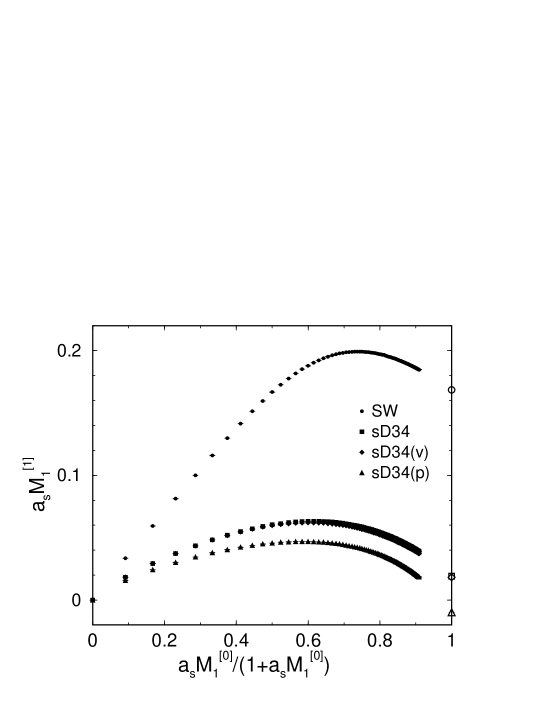
Figure 5: $a_{s}M_{1}^{[1]}$ versus $a_{s}M_{1}^{[0]}/(1+a_{s}M_{1}^{[0]})$ for the SW action and the sD34 actions. The values in the static limit are denoted by open symbols.

Now we present the results of our one-loop calculations in the $a_{t}\rightarrow 0$ limit. The one-loop correction to the rest mass $a_{s}M_{1}^{[1]}$ is plotted as a function of $a_{s}M_{1}^{[0]}/(1+a_{s}M_{1}^{[0]})$ in Figure 5, and numerical values of $a_{s}M_{1}^{[1]}$ and $a_{s}m_{0c}^{[1]}$ are given in Table 1. As shown in the figure, $a_{s}M_{1}^{[1]}$ for all the actions increase from the massless limit and reach their maximum values around $a_{s}M_{1}^{[0]}=1$–3, then decrease to the static values represented by open symbols. Fitting our results in the small mass region ($a_{s}M_{1}^{[1]}\ll 1$), we confirmed that the one-loop corrections are consistent with the mass singularity

$$M_{1}^{[1]}\sim-C_{F}\frac{3}{16\pi^{2}}M_{1}^{[0]}\log(a_{s}M_{1}^{[0]})^{2}.$$ (83)

The results for $a_{s}M_{1}^{[1]}$ in the static limit $a_{s}M_{1}^{[0]}\rightarrow\infty$ depend on the action, since the reduced static action (29) includes the $a_{s}^{3}\Delta_{i}^{2}$ term proportional to $\nu d_{s}$. This situation is in contrast to the case of finite $a_{t}$ calculations in Groote:2000jd ; Mertens:1997wx , where $a_{s}M_{1}^{[1]}$ goes to a universal value. In the finite $a_{t}$ case, $a_{s}M_{1}^{[1]}$ does not depend on $\nu d_{s}$ in the $a_{t}m_{Q}\rightarrow\infty$ limit, because the static action always gives the Wilson line.

V.2 Kinetic mass renormalization

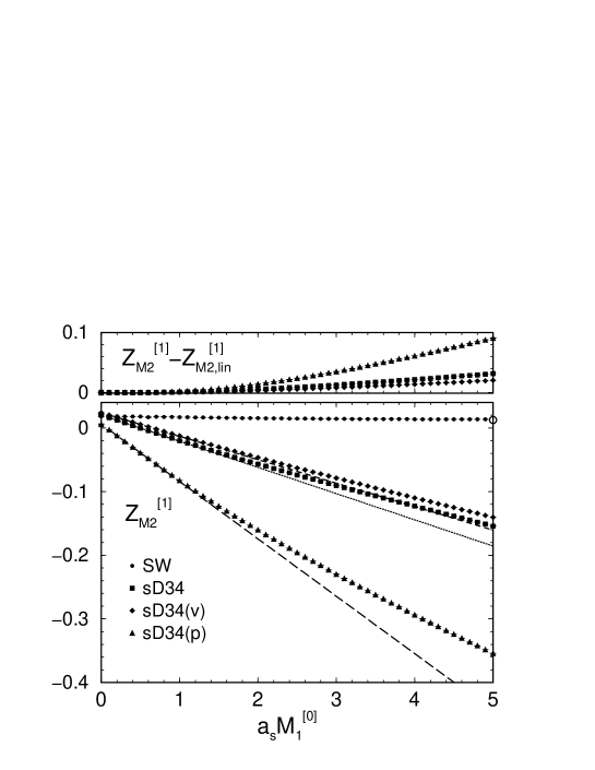
Figure 6: The lower figure shows $Z_{M_{2}}^{[1]}$ versus $a_{s}M_{1}^{[0]}$ for the SW action and the sD34 actions. The value in the static limit for the SW action is denoted by open circle. Lines are the linear approximations to the results for the sD34 actions ($Z_{M_{2},\rm lin}^{[1]}$) as explained in the text. The upper figure shows the difference $Z_{M_{2}}^{[1]}-Z_{M_{2},\rm lin}^{[1]}$ versus $a_{s}M_{1}^{[0]}$ for the sD34 actions.

The one-loop correction to the kinetic mass renormalization $Z_{M_{2}}$ is related to the speed of light renormalization $\nu$ according to (53). The study of the $a_{s}m_{Q}$ dependence of $\nu$ at the one-loop level is a main purpose of this paper. The results of $Z_{M_{2}}^{[1]}$ are shown in Figure 6, and their numerical values are given in Table 2.

First, we focus on the result for the SW action, which becomes the naive quark action in the $a_{t}\rightarrow 0$ limit as the Wilson term and the clover term vanish. From Figure 6 (lower panel), we find that the mass dependence of $Z_{M_{2}}^{[1]}$ (filled circle) is very weak, and $Z_{M_{2}}^{[1]}$ stays constant in the infinite mass limit. A difference between the value in the static limit and that in the massless limit is $Z_{M_{2}}^{[1]}(\infty)-Z_{M_{2}}^{[1]}(0)=-0.006$. This is only 6% of the same difference for the isotropic SW action $-0.10$ Mertens:1997wx . The result implies that mass dependent discretization errors of order $g^{2}(a_{s}m_{Q})^{n}$ for $Z_{M_{2}}^{[1]}$ are small on the anisotropic lattice. The same conclusion holds for any action which becomes the naive quark action in the $a_{t}\rightarrow 0$ limit. For instance, the action with $r_{s}=0$ and $d_{s}=d/\xi$, where $d$ is a constant independent of $\xi$, belongs to this class. However, we remark that such actions suffer from the spatial doublers for large values of $\xi$, as mentioned in Section II.

Next, we consider the results for the sD34 actions, which are doubler-free even in the $a_{t}\rightarrow 0$ limit. As shown in Figure 6 (lower panel), $Z_{M_{2}}^{[1]}$ for the sD34 actions monotonically decreases as the mass increases, and diverges as $O(a_{s}m_{Q})$ toward the static limit.

The $O(a_{s}m_{Q})$ divergence of $Z_{M_{2}}^{[1]}$ is due to the finiteness of $\xi D_{(1s)}$ in the static limit multiplied by $a_{s}m_{2}$ in (54). The appearance of this manifest $a_{s}m_{Q}$ dependence, which is proportional to $\nu d_{s}$, can be explained as follows. Using $Z_{M_{2}}^{[1]}$, the kinetic term renormalization $\delta_{r}$ for the static action (31) is given by

$$\delta_{r}=\lim_{m_{Q}\rightarrow\infty}\left(\frac{1}{a_{s}M_{2}}-\frac{1}{a_{s}m_{2}}\right)=-\lim_{m_{Q}\rightarrow\infty}\,g^{2}\frac{Z_{M_{2}}^{[1]}}{a_{s}m_{2}}+O(g^{4}).$$ (84)

Because $\delta_{r}$ is a constant independent of the mass, ${Z_{M_{2}}^{[1]}}$ diverges as $O(a_{s}m_{Q})$ in the large mass limit.

However, we note that this kind of $O(a_{s}m_{Q})$ divergence is nothing to do with the discretization error increasing as $a_{s}m_{Q}$ but a renormalization of the reduced static action (31). In order to isolate such an $O(g^{2}a_{s}m_{Q})$ effect, we consider a subtracted $Z_{M_{2}}^{[1]}$ defined through

$$Z_{M_{2},\rm sub}^{[1]}=Z_{M_{2}}^{[1]}+\delta_{r}^{[1]}\ a_{s}m_{2}$$ (85)

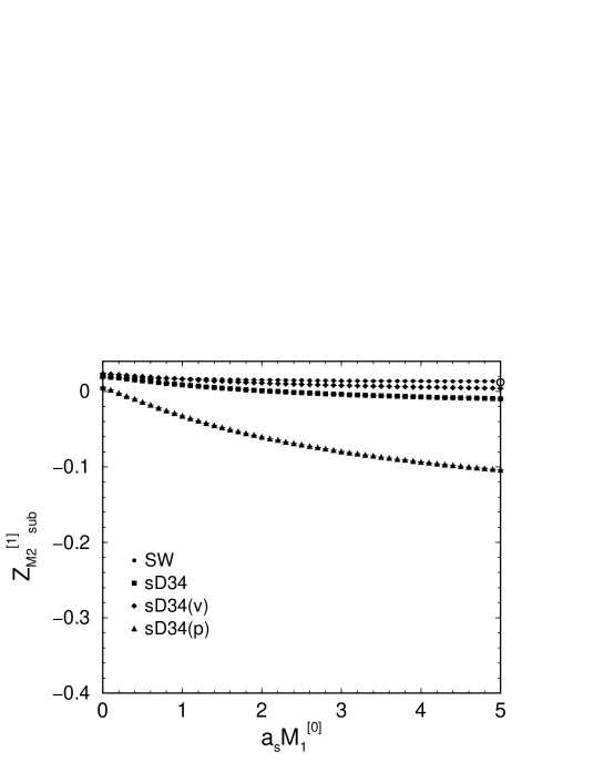
Figure 7: $Z_{M_{2},\rm sub}^{[1]}$ for the sD34 actions together with $Z_{M_{2},\rm sub}^{[1]}=Z_{M_{2}}^{[1]}$ for the SW action.

as a measure of the remaining $O(g^{2}(a_{s}m_{Q})^{n})~{}(n\geq 2)$ errors. After the subtraction of the manifest $a_{s}m_{Q}$ dependence, $Z_{M_{2},\rm sub}^{[1]}$ for the sD34 actions converges to a finite value in the static limit as shown in Figure 7. We also find that the mass dependence of $Z_{M_{2},\rm sub}^{[1]}$ for the sD34 and sD34(v) actions is as small as that for the SW action. Note that $Z_{M_{2},\rm sub}^{[1]}=Z_{M_{2}}^{[1]}$ for the SW action because of $\delta_{r}=0$.

Another way to discuss the remaining $O(g^{2}(a_{s}m_{Q})^{n})~{}(n\geq 2)$ errors for the sD34 actions is to assess their linearity in the mass parameter. Since $Z_{M_{2}}^{[1]}$ for the sD34 actions seems like a linear function of $a_{s}M_{1}^{[0]}$ effectively as shown in Figure 6 (lower panel), we attempt a linear fit using the data for $a_{s}M_{1}^{[0]}\leq 0.5$. The fitting lines $Z_{M_{2},\rm lin}^{[1]}=Z_{M_{2}}^{[1]}(0)+c_{r}^{[1]}\times\,a_{s}M_{1}^{[0]}$ shown by dashed or dotted lines approximate $Z_{M_{2}}^{[1]}$ very well from the small mass region $a_{s}M_{1}^{[0]}\ll 1$ to a relatively large mass regime $a_{s}M_{1}^{[0]}\sim 1$. The difference $Z_{M_{2}}^{[1]}-Z_{M_{2},\rm lin}^{[1]}$ is plotted in the upper panel of Figure 6. We find that the difference is less than or about 0.005 (0.01) at $a_{s}M_{1}^{[0]}=1$ (3) for the sD34 and sD34(v) actions, and slightly larger for the sD34(p) action. Since the (renormalized) coupling constant is $g^{2}=4\pi\alpha_{s}\sim 2$ in current simulations, the difference from the linearity $g^{2}(Z_{M_{2}}^{[1]}-Z_{M_{2},\rm lin}^{[1]})$ is small compared to the tree-level value $Z_{M_{2}}^{[0]}=1$. It indicates that $O(g^{2}(a_{s}m_{Q})^{n})~{}(n\geq 2)$ errors are suppressed on the anisotropic lattice, and $Z_{M_{2}}^{[1]}$ for the sD34 actions can be well approximated by a linear ansatz; $Z_{M_{2}}^{[1]}~{}\approx~{}Z_{M_{2},\rm lin}^{[1]}$.

If one would like to avoid the appearance of the renormalization scaling as $a_{s}m_{Q}$, it is possible to tune the spatial Wilson term as $R_{s}^{[1]}=-\delta_{r}^{[1]}$ such that the second term in (85) vanishes, and then the one-loop coefficient of the speed-of-light renormalization is given by $\nu^{[1]}=Z_{M_{2},\rm sub}^{[1]}/2$. Since the remaining $O((a_{s}m_{Q})^{n})$ correction for $\nu^{[1]}$ is small and does not diverge as a function of $a_{s}m_{Q}$ as shown in Figure 7, it essentially solves the problem of large radiative correction in the anisotropic lattice actions for heavy quark. It also suggests that if one can nonperturbatively tune the Wilson term in the static limit, e.g. by adjusting $r_{s}$ until the $O(a_{s}m_{Q})$ divergence of $Z_{M_{2}}$ for mesons goes away, the above cancellation of the $a_{s}m_{Q}$ error can be implemented nonperturbatively.

VI Conclusions

In this paper we discuss on the issue whether the discretization error scales as $(a_{s}m_{Q})^{n}$ when the heavy quark action is discretized on an anisotropic lattice for which the temporal lattice spacing $a_{t}$ is very small in order to keep the condition $a_{t}m_{Q}\ll 1$ while the spatial lattice spacing $a_{s}$ is relatively large and $a_{s}m_{Q}$ can be order one. Our naive expectation is that the discretization error does not behave as $a_{s}m_{Q}$ for the heavy-light mesons (or baryons) at rest, since momentum scale flowing into the spatial direction is of order of the QCD scale $\Lambda_{\mathrm{QCD}}$ rather than the heavy quark mass scale $m_{Q}$. Even at the quantum level the maximum (virtual) momentum flowing into the spatial direction is $\pi/a_{s}$, and the discretization error coming from the spatial derivative cannot pick up the large heavy quark mass.

Through the one-loop calculations of the kinetic mass renormalization for a class of lattice fermion actions, we found that our expectation is indeed the case. For the sD34 actions there is a piece which behaves as $a_{s}m_{Q}$ in the one-loop coefficient of the kinetic mass renormalization, but it originates from the renormalization of the spatial Wilson term, which remains even in the static limit, and thus does not come from the discretization of the spatial derivative. It implies that if one can nonperturbatively tune the spatial Wilson term (the parameter $r_{s}$) such that it vanishes in the static limit, the unwanted behavior $a_{s}m_{Q}$ can be removed from the speed-of-light renormalization. Although there is a possibility that the unwanted discretization error scaling as $a_{s}m_{Q}$ exists in some other quantities, it is unlikely from our considerations.

The anisotropic lattice thus remains as a promising approach to treat heavy quarks on the lattice. As in the usual relativistic approach, the theory is renormalizable and the number of necessary terms in the action is limited. It also opens a possibility to tune the parameters in the action nonperturbatively for heavy quarks.

Appendix A Definitions and Feynman rules

The lattice covariant derivatives are defined by

$$\nabla_{\mu}\psi(x) \equiv {1\over 2a_{\mu}}\,\biggl{[}U_{\mu}(x)\psi(x+\mu)-U_{-\mu}(x)\psi(x-\mu)\biggr{]}\,,$$ (86)

$$\Delta_{\mu}\psi(x) \equiv {1\over a_{\mu}^{2}}\,\biggl{[}U_{\mu}(x)\psi(x+\mu)+U_{-\mu}(x)\psi(x-\mu)-2\psi(x)\biggr{]}\,,$$ (87)

$$\nabla_{\mu}\Delta_{\mu}\psi(x) \equiv {1\over 2a_{\mu}^{3}}\,\biggl{[}U_{\mu}(x)U_{\mu}(x+\mu)\psi(x+2\mu)-U_{-\mu}(x)U_{-\mu}(x-\mu)\psi(x-2\mu)$$ (88)

$$-2U_{\mu}(x)\psi(x+\mu)+2U_{-\mu}(x)\psi(x-\mu)\biggr{]}\,,$$

$$\Delta_{\mu}^{2}\psi(x) \equiv {1\over a_{\mu}^{4}}\,\biggl{[}U_{\mu}(x)U_{\mu}(x+\mu)\psi(x+2\mu)+U_{-\mu}(x)U_{-\mu}(x-\mu)\psi(x-2\mu)$$ (89)

$$-4U_{\mu}(x)\psi(x+\mu)-4U_{-\mu}(x)\psi(x-\mu)+6\psi(x)\biggr{]}\,.$$

We also define the lattice momenta

$$a_{\mu}{\bar{p}}_{\mu} \equiv \sin(a_{\mu}p_{\mu}),$$ (90)

$$a_{\mu}\hat{p}_{\mu} \equiv 2\sin(a_{\mu}p_{\mu}/2).$$ (91)

Feynman rules for our anisotropic actions can be derived in usual way. The gluon propagator with Feynman gauge is given by

$$D_{\mu\nu}^{ab}(k)=\frac{\delta^{ab}\delta_{\mu\nu}}{\hat{k}^{2}}.$$ (92)

The quark propagator is

$$G_{0}(p)=\frac{1}{i\sum_{\mu}\gamma_{\mu}K_{\mu}(p)+L(p)},$$ (93)

where

$$K_{0}(p) = {\bar{p}}_{0}~{}\stackrel{{\scriptstyle a_{t}\rightarrow 0}}{{\longrightarrow}}~{}p_{0},$$ (94)

$$K_{i}(p) = \nu{\bar{p}}_{i}(1+b_{s}a_{i}^{2}\hat{p}_{i}^{2}),$$ (95)

and

$$L(p) = m_{0}+{1\over 2}a_{t}\sum_{\mu}r_{\mu}\hat{p}_{\mu}^{2}+\nu d_{s}\sum_{i}a_{i}^{3}\hat{p}_{i}^{4}$$ (96)

$$~{}\stackrel{{\scriptstyle a_{t}\rightarrow 0}}{{\longrightarrow}}~{} m_{0}+\nu d_{s}\sum_{i}a_{i}^{3}\hat{p}_{i}^{4}$$ (97)

for our quark actions with Eq. (8).

The one-gluon vertex with the incoming quark momentum $q$, the outgoing quark momentum $q^{\prime}$ and the incoming gluon momentum $k=q^{\prime}-q$ is given by

$$V_{1,\mu}^{a}(q,q^{\prime},k)=-igt^{a}\left[\gamma_{\mu}\bar{X}_{\mu}(q+q^{\prime},k)-i\bar{Y}_{\mu}(q+q^{\prime},k)\right],$$ (98)

where

$$\bar{X}_{\mu}(q+q^{\prime},k) = 2a_{\mu}X_{\mu}\cos\left(\frac{a_{\mu}q_{\mu}+a_{\mu}q^{\prime}_{\mu}}{2}\right)+4a_{\mu}Z_{\mu}\cos\left(a_{\mu}q_{\mu}+a_{\mu}q^{\prime}_{\mu}\right)\cos\left(\frac{a_{\mu}k_{\mu}}{2}\right),$$ (99)

$$\bar{Y}_{\mu}(q+q^{\prime},k) = 2a_{\mu}Y_{\mu}\sin\left(\frac{a_{\mu}q_{\mu}+a_{\mu}q^{\prime}_{\mu}}{2}\right)+4a_{\mu}W_{\mu}\sin\left(a_{\mu}q_{\mu}+a_{\mu}q^{\prime}_{\mu}\right)\cos\left(\frac{a_{\mu}k_{\mu}}{2}\right),$$ (100)

and

$$a_{\mu}X_{\mu} = \frac{1}{2}\,\nu_{\mu}+\nu_{\mu}b_{\mu},$$ (101)

$$a_{\mu}Y_{\mu} = \frac{1}{2}\,r_{\mu}\frac{a_{0}}{a_{\mu}}+4\nu_{\mu}d_{\mu},$$ (102)

$$a_{\mu}Z_{\mu} = -\frac{1}{2}\,\nu_{\mu}b_{\mu},$$ (103)

$$a_{\mu}W_{\mu} = -\nu_{\mu}d_{\mu}.$$ (104)

The $t^{a}$ are generators of color SU(3). We ignore the one-gluon vertex arising from the clover terms because such a vertex becomes irrelevant in the $a_{t}\rightarrow 0$ limit.

Finally the two-gluon vertex with the incoming gluon momenta $k$ and $k^{\prime}$ ($k+k^{\prime}=q^{\prime}-q$) is given by

$$V_{2,\mu\mu}^{ab}(q,q^{\prime},k,k^{\prime})=2a_{\mu}g^{2}(t^{a}t^{b})\times$$

$$\left[i\gamma_{\mu}\left\{a_{\mu}X_{\mu}\sin\left(\frac{a_{\mu}q_{\mu}+a_{\mu}q^{\prime}_{\mu}}{2}\right)+4a_{\mu}Z_{\mu}\sin\left(a_{\mu}q_{\mu}+a_{\mu}q^{\prime}_{\mu}\right)\cos\left(\frac{a_{\mu}k_{\mu}}{2}\right)\cos\left(\frac{a_{\mu}k^{\prime}_{\mu}}{2}\right)\right\}\right.$$

$$\left.-\left\{a_{\mu}Y_{\mu}\cos\left(\frac{a_{\mu}q_{\mu}+a_{\mu}q^{\prime}_{\mu}}{2}\right)+4a_{\mu}W_{\mu}\cos\left(a_{\mu}q_{\mu}+a_{\mu}q^{\prime}_{\mu}\right)\cos\left(\frac{a_{\mu}k_{\mu}}{2}\right)\cos\left(\frac{a_{\mu}k^{\prime}_{\mu}}{2}\right)\right\}\right].$$ (105)

Here we omit terms that vanish by symmetrizing between two gluons and that arise from the clover terms, which are unnecessary in the calculation of the tadpole graph.

Appendix B $k_{0}$-integrations

In this Appendix we summarize some formula on the $k_{0}$-integrations, which are needed for the calculation of the regular graph. We use the following results for one-dimensional integrations:

$$I_{1} \equiv \int^{\infty}_{-\infty}dx\,\frac{1}{a+bx^{2}}\,\frac{c}{g^{2}(ie-x)^{2}+f^{2}}$$ (106)

$$= \pi c\left\{\frac{1}{\sqrt{ab}}\,\frac{1}{-g^{2}(e-\sqrt{a/b})^{2}+f^{2}}+\frac{1}{a-b(e+f/g)^{2}}\,\frac{1}{fg}\right\},$$

$$I_{2} \equiv \int^{\infty}_{-\infty}dx\,\frac{1}{a+bx^{2}}\,\frac{c(ie-x)}{g^{2}(ie-x)^{2}+f^{2}}$$ (107)

$$= i\pi c\left\{\frac{1}{\sqrt{ab}}\,\frac{e-\sqrt{a/b}}{-g^{2}(e-\sqrt{a/b})^{2}+f^{2}}-\frac{1}{a-b(e+f/g)^{2}}\,\frac{1}{g^{2}}\right\},$$

$$I_{3} \equiv \int^{\infty}_{-\infty}dx\,\frac{1}{a+bx^{2}}\,\frac{c}{(g^{2}(ie-x)^{2}+f^{2})^{2}}~{}=~{}-\frac{1}{2f}\frac{\partial I_{1}}{\partial f},$$ (108)

$$I_{4} \equiv \int^{\infty}_{-\infty}dx\,\frac{1}{a+bx^{2}}\,\frac{c(ie-x)^{2}}{(g^{2}(ie-x)^{2}+f^{2})^{2}}~{}=~{}-\frac{1}{2g}\frac{\partial I_{1}}{\partial g},$$ (109)

$$I_{5} \equiv \int^{\infty}_{-\infty}dx\,\frac{1}{a+bx^{2}}\,\frac{c(ie-x)}{(g^{2}(ie-x)^{2}+f^{2})^{2}}~{}=~{}-\frac{1}{2f}\frac{\partial I_{2}}{\partial f},$$ (110)

$$I_{6} \equiv \int^{\infty}_{-\infty}dx\,\frac{1}{a+bx^{2}}\,\frac{c}{(g^{2}(ie-x)^{2}+f^{2})^{3}}~{}=~{}-\frac{1}{4f}\frac{\partial I_{3}}{\partial f},$$ (111)

$$I_{7} \equiv \int^{\infty}_{-\infty}dx\,\frac{1}{a+bx^{2}}\,\frac{c(ie-x)}{(g^{2}(ie-x)^{2}+f^{2})^{3}}~{}=~{}-\frac{1}{4f}\frac{\partial I_{5}}{\partial f},$$ (112)

where $e<f/g$ is assumed. These integrations are calculated by hand using the residue theorem, and checked by Mathematica.

In the calculation of the regular graph, we assign

$$x\rightarrow k_{0}\,,\ \ \ a\rightarrow|\hat{\bf k}|^{2}\,,\ \ \ b\rightarrow a_{s}^{2}\,,\ \ \ g\rightarrow 1\,,\ \ \ e\rightarrow M_{1}\,,\ \ \ f\rightarrow E({\bf k})\,,$$ (113)

where

$$E({\bf k})\equiv\sqrt{\nu^{2}\sum_{i}{\bar{k}}_{i}^{2}(1+b_{s}a_{i}^{2}\hat{k}_{i}^{2})^{2}+(m_{0}+\nu d_{s}\sum_{i}a_{i}^{3}\hat{k}_{i}^{4})^{2}}\,.$$ (114)

The overall factors $c$ depend on the spatial momentum ${\bf k}$. Using integrations $I_{1}$–$I_{7}$ with above assignments, relevant contributions from the regular graph are given by

$$\xi B_{0}^{\rm reg}(iM_{1},{\bf 0}) = \int_{\bf k}\frac{1}{2\pi}I_{2-B0}\,,$$ (115)

$$\xi C^{\rm reg}(iM_{1},{\bf 0}) = \int_{\bf k}\frac{1}{2\pi}I_{1-C}\,,$$ (116)

$$\xi A_{1}^{\rm reg}(iM_{1},{\bf 0}) = \int_{\bf k}\frac{1}{2\pi}(I_{1-A1}+I_{3-A1})\,,$$ (117)

$$\xi D_{1s}^{\rm reg}({\bf 0}) = \int_{\bf k}\frac{1}{2\pi}\left[\frac{1}{i}(I_{2-Ds}+I_{5-Ds}+I_{7-Ds})-(I_{1-Ds}+I_{3-Ds}+I_{6-Ds})\right]\,,$$ (118)

$$i\,\xi D_{1t}^{\rm reg}({\bf 0}) = \int_{\bf k}\frac{1}{2\pi}(I_{1-Dt}+I_{4-Dt}-iI_{5-Dt})\,.$$ (119)

$a_{s}M_{1}^{[1]}$
$a_{s}M_{1}^{[0]}$	SW	sD34	sD34(v)	sD34(p)
$0.0$	$0.000000(00)$	$0.000000(00)$	$0.000000(00)$	$0.000000(00)$
$0.1$	$0.033586(11)$	$0.018299(19)$	$0.018360(21)$	$0.015615(23)$
$0.2$	$0.059382(20)$	$0.029235(21)$	$0.029306(21)$	$0.024206(23)$
$0.3$	$0.081252(22)$	$0.037292(24)$	$0.037354(23)$	$0.030177(41)$
$0.4$	$0.100023(23)$	$0.043466(28)$	$0.043405(21)$	$0.034594(25)$
$0.5$	$0.116008(27)$	$0.048228(29)$	$0.048196(25)$	$0.037909(25)$
$0.6$	$0.129786(19)$	$0.051966(24)$	$0.051762(25)$	$0.040428(32)$
$0.7$	$0.141467(36)$	$0.054948(34)$	$0.054572(31)$	$0.042396(31)$
$0.8$	$0.151341(22)$	$0.057183(24)$	$0.056763(22)$	$0.043836(33)$
$0.9$	$0.159679(29)$	$0.059029(36)$	$0.058465(29)$	$0.044916(49)$
$1.0$	$0.166758(21)$	$0.060338(33)$	$0.059687(24)$	$0.045724(34)$
$2.0$	$0.196227(24)$	$0.062578(35)$	$0.060997(28)$	$0.045709(32)$
$3.0$	$0.199166(39)$	$0.058705(39)$	$0.056713(28)$	$0.041241(34)$
$4.0$	$0.197161(26)$	$0.054263(23)$	$0.052280(29)$	$0.036472(30)$
$5.0$	$0.194441(44)$	$0.050519(28)$	$0.048617(55)$	$0.032255(53)$
$10.0$	$0.184712(29)$	$0.038993(46)$	$0.037121(28)$	$0.018373(37)$
$\infty$	$0.168490(26)$	$0.019045(21)$	$0.018249(29)$	$-0.009803(27)$
$a_{s}m_{0c}^{[1]}$
-	$0.000000(00)$	$-0.060828(02)$	$-0.061672(02)$	$0.001431(03)$

Table 1: Numerical values of $a_{s}M_{1}^{[1]}$ for various values of $a_{s}M_{1}^{[0]}$, and $a_{s}m_{0c}^{[1]}$ for the SW action and the sD34 actions.

$Z_{M_{2}}^{[1]}$
$a_{s}M_{1}^{[0]}$	SW	sD34	sD34(v)	sD34(p)
$0.0$	$0.01810(35)\,\$	$0.02061(30)\,\$	$0.02369(49)\,\$	$0.00549(59)\,\$
$0.1$	$0.01812(19)\,\$	$0.016066(63)$	$0.020152(61)$	$-0.00313(11)\,\$
$0.2$	$0.018236(53)$	$0.012019(46)$	$0.016416(46)$	$-0.012140(85)$
$0.3$	$0.017991(51)$	$0.007856(48)$	$0.012592(45)$	$-0.021208(59)$
$0.4$	$0.017941(49)$	$0.003750(39)$	$0.009003(38)$	$-0.030040(78)$
$0.5$	$0.017801(43)$	$-0.000349(34)$	$0.005406(47)$	$-0.039223(56)$
$0.6$	$0.016708(38)$	$-0.004308(39)$	$0.001676(33)$	$-0.047996(50)$
$0.7$	$0.017507(32)$	$-0.008387(32)$	$-0.001963(32)$	$-0.056888(53)$
$0.8$	$0.017326(64)$	$-0.012299(84)$	$-0.005543(28)$	$-0.065500(50)$
$0.9$	$0.017142(47)$	$-0.016238(28)$	$-0.009117(28)$	$-0.074070(46)$
$1.0$	$0.016862(36)$	$-0.020149(28)$	$-0.012661(31)$	$-0.082456(55)$
$2.0$	$0.015176(35)$	$-0.056742(34)$	$-0.046665(28)$	$-0.160259(59)$
$3.0$	$0.014246(21)$	$-0.090607(29)$	$-0.078766(30)$	$-0.229675(78)$
$4.0$	$0.013677(17)$	$-0.122890(42)$	$-0.109982(40)$	$-0.293550(90)$
$5.0$	$0.013371(18)$	$-0.154177(45)$	$-0.140336(48)$	$-0.35409(12)\,\$
$10.0$	$0.012716(15)$	$-0.304675(91)$	$-0.288888(86)$	$-0.63276(22)\,\$
$\infty$	$0.012316(07)$	$-\infty$	$-\infty$	$-\infty$

Table 2: Numerical values of $Z_{M_{2}}^{[1]}$ for the SW action and the sD34 actions.

Figure 1: Energy-momentum relation at different values of $\xi$ for the SW action. The left panel shows the case of $a_{s}E({\bf 0})=0$, while the right shows $a_{s}E({\bf 0})=1$. The spatial momentum ${\bf p}$ is along the $(1,1,0)$ direction. For comparison we also plot the energy-momentum relation in the continuum.

Figure 2: Energy-momentum relation for the sD34 action.

Figure 3: Energy-momentum relation for the sD34(p) action.

Figure 4: Feynman graphs relevant for the one-loop quark self energy. The left (a) is the regular graph, and the right (b) is the tadpole graph.

References

- (1) N. Yamada, review talk at 20th International Symposium on Lattice Field Theory (LATTICE 2002), Boston, Massachusetts, 24-29 Jun 2002; arXiv:hep-lat/0210035.
- (2) B. A. Thacker and G. P. Lepage, Phys. Rev. D 43, 196 (1991).
- (3) G. P. Lepage, L. Magnea, C. Nakhleh, U. Magnea and K. Hornbostel, Phys. Rev. D 46, 4052 (1992) [arXiv:hep-lat/9205007].
- (4) A. X. El-Khadra, A. S. Kronfeld and P. B. Mackenzie, Phys. Rev. D 55, 3933 (1997) [arXiv:hep-lat/9604004].
- (5) M. G. Alford, T. R. Klassen and G. P. Lepage, Nucl. Phys. B 496, 377 (1997) [arXiv:hep-lat/9611010].
- (6) T. R. Klassen, Nucl. Phys. Proc. Suppl. 73, 918 (1999) [arXiv:hep-lat/9809174]; T. R. Klassen, unpublished.
- (7) J. Harada, A. S. Kronfeld, H. Matsufuru, N. Nakajima and T. Onogi, Phys. Rev. D 64, 074501 (2001) [arXiv:hep-lat/0103026].
- (8) S. Aoki, Y. Kuramashi and S. Tominaga, arXiv:hep-lat/0107009.
- (9) B. Sheikholeslami and R. Wohlert, Nucl. Phys. B 259, 572 (1985).
- (10) T. Umeda, R. Katayama, O. Miyamura and H. Matsufuru, arXiv:hep-lat/0011085.
- (11) H. Matsufuru, T. Onogi and T. Umeda, Phys. Rev. D 64, 114503 (2001) [arXiv:hep-lat/0107001].
- (12) J. Harada, H. Matsufuru, T. Onogi and A. Sugita, Phys. Rev. D 66, 014509 (2002) [arXiv:hep-lat/0203025].
- (13) H. W. Hamber and C. M. Wu, Phys. Lett. B 133, 351 (1983).
- (14) T. Eguchi and N. Kawamoto, Nucl. Phys. B 237, 609 (1984).
- (15) P. Chen, Phys. Rev. D 64, 034509 (2001) [arXiv:hep-lat/0006019].
- (16) M. Okamoto et al. [CP-PACS Collaboration], Phys. Rev. D 65, 094508 (2002) [arXiv:hep-lat/0112020].
- (17) Z. H. Mei and X. Q. Luo, arXiv:hep-lat/0206012.
- (18) S. Groote and J. Shigemitsu, Phys. Rev. D 62, 014508 (2000) [arXiv:hep-lat/0001021].
- (19) S. Collins, C. T. Davies, J. Hein, R. R. Horgan, G. P. Lepage and J. Shigemitsu [UKQCD collaboration], Phys. Rev. D 64, 055002 (2001) [arXiv:hep-lat/0101019].
- (20) J. Shigemitsu, S. Collins, C. T. Davies, J. Hein, R. R. Horgan and G. P. Lepage, arXiv:hep-lat/0207011.
- (21) B. P. Mertens, A. S. Kronfeld and A. X. El-Khadra, Phys. Rev. D 58, 034505 (1998) [arXiv:hep-lat/9712024].
- (22) G. P. Lepage and P. B. Mackenzie, Phys. Rev. D 48, 2250 (1993) [arXiv:hep-lat/9209022].
- (23) G. P. Lepage, J. Comput. Phys. 27, 192 (1978).