Duality of gauge field singularities and the structure of the flux tube in Abelian-projected SU(2) gauge theory and the dual Abelian Higgs model

Abstract

The structure of the flux-tube profile in Abelian-projected (AP) SU(2) gauge theory in the maximally Abelian gauge is studied. The connection between the AP flux tube and the classical flux-tube solution of the U(1) dual Abelian Higgs (DAH) model is clarified in terms of the path-integral duality transformation. This connection suggests that the electric photon and the magnetic monopole parts of the Abelian Wilson loop can act as separate sources creating the Coulombic and the solenoidal electric field inside a flux tube. The conjecture is confirmed by a lattice simulation which shows that the AP flux tube is composed of these two contributions.

I Introduction

When the QCD vacuum is viewed as a dual superconductor tHooft:1975pu ; Mandelstam:1974pi , the quark confinement mechanism can be immediately understood: the (color-) electric flux associated with a quark-antiquark ($q$-$\bar{q}$) system is squeezed into an almost-one-dimensional flux tube by the dual Meissner effect caused by magnetic monopole condensation. This picture leads to a linear confinement potential and is a dual analogue of the magnetic Abrikosov vortex in an ordinary superconductor Abrikosov:1957sx ; Nielsen:1973ve ; Nambu:1974zg . It is natural to expect that it can be quantitatively formulated by a dual version of an Abelian Higgs model, the dual Abelian Higgs (DAH) model. The Lagrangian — besides the kinetic terms of each field and a minimal coupling between the two fields — should contain a monopole self-interaction term that allows for a broken phase of dual gauge symmetry. The DAH model indeed has an electric flux-tube solution of the static $q$-$\bar{q}$ system Nambu:1974zg .

A linear potential emerging from a flux tube is quite welcome to give an interpretation for the area law behavior of the Wilson loop observed in lattice QCD simulations Creutz:1984mg . It would explain the Regge trajectory pattern or other string-like properties of hadrons Sailer:1991jv . Then the problem arises how to derive the dual superconductor scenario from QCD, that is, how to formally derive the DAH model from QCD. One also would like to observe certain characteristic features of the dual superconductor, such as the formation of flux tubes, through a Monte-Carlo simulation of lattice QCD directly.

As for the formal derivation, it is known that if magnetic monopoles are introduced as the consequence of Abelian projection a la ’t Hooft tHooft:1981ht and if the diagonal components of gluons play a dominant role (compared to the off-diagonal ones) in the long distance behavior of QCD (Abelian dominance), a condensed phase of monopoles is realized beyond a certain critical scale Ezawa:1982bf ; Ezawa:1982ey . Remarkably, lattice QCD simulations with non-Abelian configurations undergoing ’t Hooft’s Abelian-projection (typically in the maximally Abelian gauge, MAG) support this scenario numerically. For instance, the string tension measured by the “Abelian Wilson loop” constructed from the Abelian link variables (the “Abelian string tension”), is almost saturating the non-Abelian string tension Suzuki:1990gp . In this context, applying the Zwanziger formalism Zwanziger:1971hk , one can introduce the dual gauge field which is minimally coupled to monopoles. Summing over monopole current trajectories Bardakci:1978ph ; Stone:1978mx , one can also introduce a monopole field. This formulation finally leads to the DAH model Suzuki:1988yq ; Maedan:1988yi ; Suganuma:1995ps ; Sasaki:1995sa . However, it is difficult to determine the effective couplings of the DAH model through this analytical derivation, because one cannot treat the monopole current system quantitatively. In order to accomplish this, one would need numerical investigations of monopole dynamics on the lattice, for instance by means of the inverse Monte-Carlo method Shiba:1995pu ; Shiba:1995db ; Kato:1998ur ; Chernodub:2000ax . This might require more complicated ansätze for matching the monopole actions Suzuki:2001tp .

Just in order to seek flux-tube configurations in the non-Abelian gauge theory, the profiles of the electric field and the monopole current distribution induced by an Abelian Wilson loop have been studied within the Abelian-projection scheme Singh:1993jj ; Matsubara:1994nq ; Cea:1995zt ; Bali:1998gz . It has been found that the shapes are similar to those of the flux-tube solution in the DAH model. From now we call the former one “Abelian-projected (AP) flux tube” and the latter one “DAH flux tube”. We remark that the connection between the AP flux tube and the DAH flux tube is not on equal footing because the former contains the quantum effects at work in non-Abelian lattice gauge simulations on the original lattice, while the latter is a classical solution obtained by solving the field equations with dual variables. Having in mind this conceptual difference, it is still worth to determine the effective couplings of the DAH model, which could not be fixed through a formal derivation, through the comparison between the two flux tubes. This is interesting because, once the DAH parameters are fixed, one can use the DAH model for further analyses: for discussing hadronic objects Kamizawa:1993hb ; Koma:1999sm ; Koma:2000hw , for investigating the dynamics of the flux tube by deriving an effective string action from the DAH model Akhmedov:1996mw ; Antonov:1998xt ; Antonov:1998wi ; Chernodub:1998ie ; Koma:2001pz ; Koma:2002rw , etc.

Up to now, the quantitative status of the comparison between the AP and the DAH flux tubes has not been conclusive, although this has been attempted several times Singh:1993jj ; Matsubara:1994nq ; Cea:1995zt ; Bali:1998gz ; Gubarev:1999yp . In order to find DAH parameters which possess physical meaning in this context, at first it is important to understand to what extent the AP flux tube can be really related to the DAH flux tube, first of all since they are defined in terms of different (original and dual) variables. This should become clear once the duality transformation is carried out in detail. Second, also a more systematic study of the AP flux-tube profile is required to have well-controlled lattice data; one needs to check the Gribov copy effect hidden in the process of MAG fixing, has to examine to what extent the scaling property is fulfilled, should investigate the $q$-$\bar{q}$ distance dependence of the flux tube shape etc. on a sufficiently large lattice volume.

In this paper, we aim to address only the first part, the qualitative and detailed relation between the AP and the DAH flux tubes. Here we do not attempt to fix the DAH model parameters. What we plan to do here is to show that the AP flux tube has the composed internal structure as the DAH flux tube has, going through the path-integral duality transformation of the AP gauge theory. In fact, in the DAH model, as we explain later in detail, the appearance of the electric flux tube is due to the superposition of two well distinguished components, a Coulombic electric field, directly induced by the electric charges, and a solenoidal electric field induced by a monopole supercurrent. They are responsible for the Coulombic and the linearly rising part, respectively, of the inter-quark potential in the DAH model. If the electric flux profile can be uniquely decomposed in the case of the AP flux tube as well, analogously to the DAH flux tube, this will be an additional argument in favor of the DAH model description, which will be important for further quantitative discussions.

The guiding idea to discover this kind of structure also in the AP flux tube comes from the measurement of the $q$-$\bar{q}$ potential in terms of the Abelian Wilson loop. The investigation of the Abelian Wilson loop using the decomposition into an electric photon part (“photon Wilson loop”) and a magnetic monopole part (“monopole Wilson loop”) shows that also the Abelian potential consists of a Coulombic and a linear potential Stack:1994wm ; Shiba:1994ab ; Bali:1996dm . We notice that this structure is quite similar to that of the $q$-$\bar{q}$ potential in the DAH model.

The paper is organized as follows. In section II we shall discuss the theoretical connection of the photon and the monopole Wilson loops with the composed structure of the DAH flux tube. We do this by closely looking at the path-integral duality transformation of the AP gauge theory. Motivated by lattice results on the effective monopole action we adopt, as our starting point, a Villain type compact QED as the approximate action of the effective, AP gauge theory. In section III we present the numerical results, the flux profile induced by the photon and monopole Wilson loops, measured within SU(2) lattice gauge theory in the MAG. We come to the conclusion that the AP flux tube is composed out of Coulomb and solenoidal parts, which add up to the full electric flux tube, in the same manner as the DAH flux tube. Section IV is the summary.

The due improvement in the systematic study of the AP flux tube including all details of the quantitative analysis of our lattice data, along the guiding lines formulated in the present paper, is the subject of our follow-up paper koma-next .

II The composed structure of the flux tube in the DAH model

In this section, based on a path-integral analysis, we discuss a possible theoretical relation between the electric-photon and magnetic-monopole parts of the Abelian Wilson loop in the AP-SU(2) lattice gauge theory and the composed internal structure of the flux-tube solution in the U(1) DAH model.

From lattice studies of the effective monopole action in the MAG Shiba:1995pu ; Shiba:1995db ; Kato:1998ur ; Chernodub:2000ax , it is numerically suggested that, at some infrared scale, the partition function of the AP-SU(2) theory is represented by the Villain type modification of compact QED. Thus, we regard it as the effective AP gauge theory and start from the partition function

$${\cal Z}=\int_{-\pi}^{\pi}{\cal D}\theta\sum_{n^{(m)}\in Z\!\!\!Z}\exp\left[-\frac{1}{2}(F,\Delta D\;F)+i(\theta,j)\right]\;.$$ (1)

$F(C_{2})$ is the field strength

$$F=d\theta-2\pi n^{(m)}\;,$$ (2)

which is composed of compact link variables, $\theta(C_{1})\in[-\pi,\pi)$, and magnetic Dirac strings, $n^{(m)}(C_{2})\in Z\!\!\!Z$ Chernodub:1997ay . $\theta$ corresponds to the Abelian gauge field, which interacts with an external electric current $j(C_{1})\in Z\!\!\!Z$. The operator $D$ is a general differential operator and $\Delta$ is the Laplacian on the lattice. In the infrared limit, it is numerically shown that the operator $D$ is well-described by the following form: $D=\beta_{e}\Delta^{-1}+\alpha+\gamma\Delta$, where $\beta_{e}$, $\alpha$ and $\gamma$ are renormalized coupling constants of the monopole action which satisfy the relation $\beta_{e}\gg\alpha$, $\gamma$ Suzuki:2002sr . The (inverse) effective gauge coupling is $\beta_{e}\equiv 4/e^{2}$. Since the magnetic Dirac strings $n^{(m)}$ are bordered by magnetic monopole currents $k(C_{3})$ as $dn^{(m)}=-k$ (hence $dk=0$), the Abelian Bianchi identity is now violated as $dF=-2\pi\;dn^{(m)}=2\pi k$.

For a conserved electric current, $\delta j=0$, we call

$$W_{A}[j]\equiv\exp[i(\theta,j)]$$ (3)

the Abelian Wilson loop. Its electric-photon ($W_{\mathit{Ph}}$) and the magnetic-monopole ($W_{\mathit{Mo}}$) parts are specified as follows. Applying the Hodge decomposition to $\theta$, we have the relation

$$\theta = \Delta^{-1}\Delta\theta$$ (4)

$$= \Delta^{-1}(\delta d+d\delta)\theta$$

$$= \Delta^{-1}\delta F+2\pi\Delta^{-1}\delta n^{(m)}+\Delta^{-1}d\delta\theta$$

$$= \Delta^{-1}\delta F+2\pi\Delta^{-1}\delta p+2\pi q+\Delta^{-1}d\delta(\theta-2\pi q).$$

In the last line, we have used the relation $n^{(m)}=p+dq$, where $p(C_{2}),\;q(C_{1})\in Z\!\!\!Z$. This means that an arbitrary shape of the open magnetic Dirac string $n^{(m)}$ is in general described by the sum of a fixed open string $p$ with $dp=-k$ and the closed strings $dq$ with $d^{2}q=0$. Since all possible closed string fluctuations are summed over, one can choose an arbitrary open string $p$. Inserting Eq. (4) into Eq. (3), the Abelian Wilson loop can be written as

$$W_{A}[j]=\exp[i(\Delta^{-1}\delta F,j)]\cdot\exp[i(2\pi\Delta^{-1}\delta p,j)]=W_{\mathit{Ph}}[j]\cdot W_{\mathit{Mo}}[j],$$ (5)

where the third and fourth terms of Eq. (4) do not contribute to this decomposition because of the relations $\exp[2\pi i(q,j)]=1$ and $\delta j=0$.

Let us proceed with the path integration of the partition function (1) keeping track of the two parts of the Wilson loop, $W_{\mathit{Ph}}[j]$ and $W_{\mathit{Mo}}[j]$. For simplicity and for picking up the essence of the following discussions, we restrict the differential operator in Eq. (1) to the leading term, $D=\beta_{e}\Delta^{-1}$. The path integral duality transformation of such a model itself has been discussed in many places since the works Banks:1977cc ; Peskin:1978kp .

We first rewrite the summation over Dirac strings as the independent summation over monopole currents $k$ (with constraint $dk=0$) and $q$ as

$$\sum_{n^{(m)}\in Z\!\!\!Z}=\sum_{k\in Z\!\!\!Z,\;dk=0}\;\sum_{q\in Z\!\!\!Z}\;.$$ (6)

Then, the integration with respect to $\theta$ is replaced by

$$\int_{-\pi}^{\pi}{\cal D}\theta\sum_{q\in Z\!\!\!Z}=\int_{\infty}^{\infty}{\cal D}\theta^{ph}\;,$$ (7)

where $\theta^{ph}=\Delta^{-1}\delta F$ represent noncompact link variables. Acting with an exterior derivative on $\theta^{mo}=2\pi\Delta^{-1}\delta p$, one finds $d\theta^{mo}=2\pi(n^{(m)}+C^{(m)}-dq)$ with $C^{(m)}=\Delta^{-1}\delta k$. Thus, the partition function is written as noncompact QED with summation over closed monopole currents,

$${\cal Z}=\int_{-\infty}^{\infty}{\cal D}\theta^{ph}\sum_{k\in Z\!\!\!Z,\;dk=0}\exp\left[-\frac{\beta_{e}}{2}(d\theta^{ph}+2\pi C^{(m)})^{2}+i(\theta^{ph}+\theta^{mo},j)\right]\;.$$ (8)

In this expression one still realizes the violation of Abelian Bianchi identity in the form $dF=2\pi dC^{(m)}=2\pi k$ due to $dC^{(m)}=k$. Using the relation $(d\theta^{ph},C^{(m)})=(\theta^{ph},\delta C^{(m)})=0$ (since $\delta C^{(m)}=0$) one can write $(F)^{2}=(d\theta^{ph})^{2}+4\pi^{2}(C^{(m)})^{2}$. Taking into account the gauge fixing condition $\delta\theta^{ph}=0$, one can integrate over $\theta^{ph}$. This yields a direct interaction term between electric currents $j$ via the Coulomb propagator $\Delta^{-1}$. Thus we have

$${\cal Z} = \sum_{k\in Z\!\!\!Z,\;dk=0}\!\exp\left[-\frac{1}{2\beta_{e}}(j,\Delta^{-1}j)-2\pi^{2}\beta_{e}(C^{(m)})^{2}+i(\theta^{mo},j)\right]\;.$$ (9)

Defining $C^{(e)}({}^{*\!}C_{2})\equiv\Delta^{-1}\delta*j$ in analogy to $C^{(m)}=\Delta^{-1}\delta k$, the first term of the action can also be written in the form

$$\frac{1}{2\beta_{e}}(j,\Delta^{-1}j)=\frac{1}{2\beta_{e}}(*j,\Delta^{-1}*j)=\frac{1}{2\beta_{e}}(C^{(e)})^{2}=2\pi^{2}\beta_{m}(C^{(e)})^{2}\;,$$ (10)

where we have introduced the (inverse) dual gauge coupling $\beta_{m}=1/g^{2}$, which should satisfy $4\pi^{2}\beta_{e}\beta_{m}=1$ (i.e. Dirac’s condition $eg=4\pi$). Similarly, the square of $C^{(m)}$ can be rewritten

$$2\pi^{2}\beta_{e}(C^{(m)})^{2}=\frac{1}{2\beta_{m}}(k,\Delta^{-1}k)=\frac{1}{2\beta_{m}}(*k,\Delta^{-1}*k)\;.$$ (11)

The exponential of this expression can further be understood as resulting from functional integration over the magnetic part of a noncompact dual gauge field $\tilde{\theta}^{mo}({}^{*\!}C_{1})$, minimally coupled to the magnetic monopole current,

$$\exp\left[-\frac{1}{2\beta_{m}}(*k,\Delta^{-1}*k)\right]=\int_{-\infty}^{\infty}{\cal D}\tilde{\theta}^{mo}\exp\left[-\frac{\beta_{m}}{2}(d\tilde{\theta}^{mo})^{2}+i(\tilde{\theta}^{mo},*k)\right]\;.$$ (12)

We have attached the superscript “ ^mo ” in order to distinguish it from the photon part of the dual gauge field, $\tilde{\theta}^{ph}({}^{*\!}C_{1})$, which is defined in analogy to $\theta^{mo}$ as

$$\tilde{\theta}^{ph}=2\pi\Delta^{-1}\delta n^{(e)}.$$ (13)

Here $n^{(e)}({}^{*\!}C_{2})\in Z\!\!\!Z$ denotes electric Dirac strings, satisfying $dn^{(e)}=-*j$, which necessarily accompanies the presence of external electric charges. Formally, $\tilde{\theta}^{ph}$ enters our consideration when we re-express the monopole Wilson loop, using the relation

$$(\theta^{mo},j)-(\tilde{\theta}^{ph},*k)=-2\pi(p,*n^{(e)})=2\pi N\qquad(N\in Z\!\!\!Z)\;.$$ (14)

This means that the direct coupling of $j$ to $\theta^{mo}$ can be set equal to that of $k$ to $\tilde{\theta}^{ph}$, because of $\exp[i(2\pi N)]=1$. Thus, the partition function is found to be

$${\cal Z}=\int_{-\infty}^{\infty}{\cal D}\tilde{\theta}^{mo}\sum_{k\in Z\!\!\!Z,\;dk=0}\exp\Biggl{[}-\frac{\beta_{m}}{2}(d\tilde{\theta}^{mo}+2\pi C^{(e)})^{2}+i(\tilde{\theta}^{mo}+\tilde{\theta}^{ph},*k)\Biggl{]}\;.$$ (15)

The action is invariant under the transformation $\tilde{\theta}^{mo}\mapsto\tilde{\theta}^{mo}+d\tilde{f}$. This is nothing but the realization of the dual gauge symmetry, due to the conservation of magnetic monopole currents, $dk=0$. In this action, the electric currents are now implicitly defined via the violation of the dual Abelian Bianchi identity written down for the dual field strength

$$\tilde{F}=d\tilde{\theta}^{mo}+2\pi C^{(e)}$$ (16)

as $d\tilde{F}=2\pi dC^{(e)}=2\pi*j$, where $dC^{(e)}=*j$.

The summation over monopole currents is the most difficult part of the evaluation. In principle, one needs to know the monopole dynamics, for instance, such as monopole current distribution in the vacuum and self interactions, etc. The numerical investigations of the effective monopole actions based on lattice Monte-Carlo simulation in the MAG provide such information, which has suggested the approximate form of the AP action given in Eq. (1). Here, we are not going to deal with these complication, since the kinetic structure of the dual gauge field, being composed of a regular $\tilde{\theta}^{mo}$ and a singular $\tilde{\theta}^{ph}$ parts, is not affected by the summation over monopoles. We then assume that the monopole current system is described by the grand canonical ensemble of closed loops, interacting via the dual gauge field. Then the complex-valued scalar monopole field $\chi$, which minimally couples to the dual gauge field, is introduced Bardakci:1978ph ; Stone:1978mx instead of monopole currents as

$$\sum_{k\in Z\!\!\!Z,\;dk=0}\exp\Biggl{[}i(\tilde{\theta}^{mo}+\tilde{\theta}^{ph},*k)\Biggl{]}\to\int{\cal D}\chi{\cal D}\chi^{*}\exp\Biggl{[}-\left\{|(d+i(\tilde{\theta}^{mo}+\tilde{\theta}^{ph}))\chi|^{2}+\lambda(|\chi|^{2}-v^{2})^{2}\right\}\Biggl{]},$$ (17)

where the $\lambda|\chi|^{4}$ ($\lambda>0$) term plays the role to keep the density of loops being finite (it produces a short distance repulsion between the loop segments) and $v$ denotes monopole condensate which describes the typical scale of the system. In this way, we arrive at the DAH model,

$$S_{\rm DAH}=\frac{\beta_{m}}{2}(\tilde{F})^{2}+|(d+i(\tilde{\theta}^{mo}+\tilde{\theta}^{ph}))\chi|^{2}+\lambda(|\chi|^{2}-v^{2})^{2}.$$ (18)

Although we cannot argue the precise values of the effective couplings in this formal derivation, we can restrict ourselves to the range of parameters able to describe the condensed phase of monopoles, according to the lattice results Shiba:1995db .

Due to the singular structure of $\tilde{\theta}^{ph}$ associated with $n^{(e)}$ (see, Eq. (13)), the DAH model has the open flux-tube solution, obtained by solving the field equations,

$$\beta_{m}\partial_{\mu}(\partial_{\mu}\tilde{\theta}_{\nu}^{mo}-\partial_{\nu}\tilde{\theta}_{\mu}^{mo})=2(\tilde{\theta}_{\nu}^{mo}+\tilde{\theta}_{\nu}^{ph})\phi^{2}=k_{\nu}\;,$$ (19)

$$\partial_{\mu}\partial_{\mu}\phi+(\tilde{\theta}_{\mu}^{mo}+\tilde{\theta}_{\mu}^{ph})^{2}\phi=2\lambda\phi(\phi^{2}-v^{2})\;.$$ (20)

Here, we have inserted the polar decomposition of the monopole field $\chi=\phi\exp(i\eta)$ ($\phi,\eta\in\Re$), and the phase $\eta$ has been absorbed into the definition of $\tilde{\theta}_{\mu}^{mo}$. The boundary conditions of the dual gauge field and monopole field are determined so as to make the energy of the system finite: just on the electric Dirac string $n^{(e)}$, $\tilde{\theta}^{mo}_{\mu}=0$ and $\phi=0$ whereas at large distance from the string, $\tilde{\theta}^{mo}_{\mu}=-\tilde{\theta}^{ph}_{\mu}$ and $\phi=v$. After solving the field equations (in general, numerically), we can compute the profile of the electric field as the spatial part of the field strength $\tilde{F}$ in Eq. (16),

$$E = \mbox{\boldmath$\nabla$}\times\tilde{\mbox{\boldmath$\theta$}}^{mo}+2\pi\mbox{\boldmath$C$}^{(e)}\equiv\mbox{\boldmath$E$}^{mo}+\mbox{\boldmath$E$}^{ph},$$ (21)

and the magnetic current as the spatial part of the monopole current,

$$k = 2(\tilde{\mbox{\boldmath$\theta$}}^{mo}+\tilde{\mbox{\boldmath$\theta$}}^{ph})\phi^{2},$$ (22)

respectively. Concrete forms of the field equations and the boundary conditions of fields for the straight $q$-$\bar{q}$ system are given in the Appendix A.

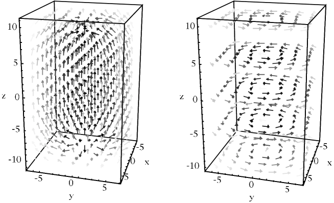
Figure 1: Profiles of electric field $\mbox{\boldmath$E$}\cdot a^{2}$ (left) and monopole current $\mbox{\boldmath$k$}\cdot a^{3}$ (right) in the DAH model, where $a$ denotes a certain length scale.

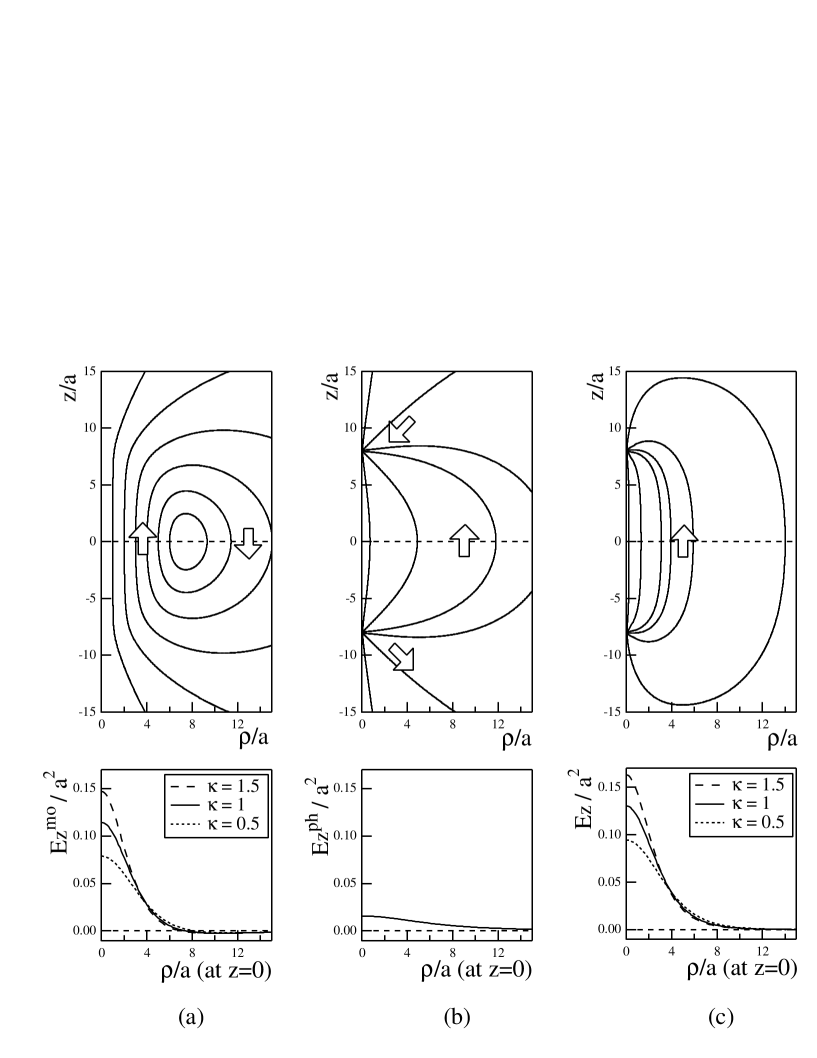
Figure 2: The flux-line pattern of the electric field (upper row) and the electric field strength as a function of the cylindrical radius (lower row): (a) the solenoidal electric field $\mbox{\boldmath$E$}^{mo}$ and (b) the Coulombic field $\mbox{\boldmath$E$}^{ph}$ add up to the flux-tube profile of the full electric field (c).

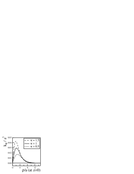
Figure 3: The monopole current strength as a function of the cylindrical radius.

A typical flux-tube solution, the profile of the electric field and the monopole current, for the straight $q$-$\bar{q}$ system is shown in Fig. 1. The parameters we have chosen are $\beta_{m}=1/g^{2}=1$, $m_{B}\cdot a=\sqrt{2}gv\cdot a=0.5$ and $m_{\chi}\cdot a=2\sqrt{\lambda}v\cdot a=0.5$, taking the $q$-$\bar{q}$ separation $r=16\;a$, where $a$ is a certain length scale. The Ginzburg-Landau parameter is here $\kappa\equiv m_{\chi}/m_{B}=1$, which means the vacuum has superconducting properties just between type-I and type-II vacuum. This set of parameters is just to illustrate the flux-tube profile as an example. In Fig. 2, we then show the ingredient of the electric-field profile based on Eq. (21). We plot the flux-line pattern of the electric fields along the $q$-$\bar{q}$ axis, and the strength of each field as a function of the cylindrical radius. In Fig. 3, we plot the strength of azimuthal monopole-current profile. Here, for the plots of the electric field and monopole current, we have added two cases corresponding to $m_{B}\cdot a=0.5$ and $m_{\chi}\cdot a=0.25$ ($\kappa=0.5$ : type I) and $m_{B}\cdot a=0.5$ and $m_{\chi}\cdot a=0.75$ ($\kappa=1.5$ : type II). Note that only the monopole-related part depends on $\kappa$, while the photon part does not.

In Fig. 2, we find that although the electric field derived from the monopole part of the dual gauge field, $E_{z}^{mo}$, takes positive value near the center, it turns negative beyond a certain radius $\rho_{c}$ (in the given case, $\rho_{c}\sim 7a$): this signals the appearance of a solenoidal electric field which plays an important role to cancel the Coulombic field, $E_{z}^{ph}$, induced by electric charges, at some distance from the electric Dirac string. By this interplay the total electric field is squeezed from the dual superconducting vacuum, which finally leads to a flux tube. This is the composed internal structure of the DAH flux tube we are referring to. The solenoidal electric field and monopole supercurrent are related by the relation, $\mbox{\boldmath$\nabla$}\times\mbox{\boldmath$E$}^{mo}=\mbox{\boldmath$k$}$. It is important to realize that although the shape of total electric field profile becomes steeper as increasing $\kappa$ due to the change of its monopole part, the flux tube is always composed of the Coulombic and solenoidal electric fields. For the infinitely separated $q$-$\bar{q}$ system, the Coulombic contribution disappears and only the solenoidal electric field remains, where translational invariance of the flux-tube profile along the $q$-$\bar{q}$ axis becomes manifest.

Now we come to the main point of the present section. Through the path-integral duality transformation, which has formally led us to the DAH model, we have found the role of the photon Wilson loop $W_{\mathit{Ph}}[j]=\exp[i(\theta^{\mathit{ph}},j)]$ and the monopole Wilson loop $W_{\mathit{Mo}}[j]=\exp[i(\theta^{\mathit{mo}},j)]$ for the DAH model and its flux-tube solution; $W_{\mathit{Ph}}[j]$ leads to the square of the Coulombic field strength $C^{(e)}$ after the integration over $\theta^{ph}$ (see, Eq. (10)), while $W_{\mathit{Mo}}[j]$ is translated into the interaction term between $\tilde{\theta}^{ph}=2\pi\Delta^{-1}\delta n^{(e)}$ and the monopole field $\chi$ (see, Eqs. (14) and (17)). Namely, the photon Wilson loop provides the origin of the Coulombic electric field contribution to the DAH flux tube. On the other hand, the monopole Wilson loop determines the non-trivial behavior of the dual gauge field, inducing the monopole supercurrent and the solenoidal electric field component of the DAH flux tube. The Coulombic and solenoidal electric fields are responsible for the Coulombic and linearly rising parts of the inter-quark potential in the DAH model. In the actual AP lattice gauge simulations, it has been numerically shown that the potential detected by the photon and monopole Wilson loops have just the same feature Stack:1994wm ; Shiba:1994ab ; Bali:1996dm . Now, this is naturally understood from the relation between each Wilson loop and the composed internal structure of the DAH flux tube. We then expect that the AP flux tube will exhibit the same composed structure as in the DAH flux tube, where $W_{\mathit{Ph}}[j]$ and $W_{\mathit{Mo}}[j]$ would be respective sources.

III Detecting the composed structure of Abelian-projected flux tube

In this section, we are going to confirm the composed structure of the AP flux tube by measuring the electric field and monopole current profiles induced from the photon and monopole parts of the Abelian Wilson loop, based on the Monte-Carlo simulation of SU(2) lattice gauge theory in the MAG.

In order to measure the the flux-tube profile induced by the Abelian Wilson loop $W_{A}[j]=\exp[i(\theta,j)]$, one can schematically use the following relation for a local operator ${\cal O}$:

$$\langle{\cal O}\rangle_{j} = \frac{\int_{-\pi}^{\pi}{\cal D}\theta\sum_{n^{(m)}}\;{\cal O}\;\exp\left[-\frac{1}{2}(F,\Delta DF)+i(\theta,j)\right]}{\int_{-\pi}^{\pi}{\cal D}\theta\sum_{n^{(m)}}\;\exp\left[-\frac{1}{2}(F,\Delta DF)+i(\theta,j)\right]}$$ (23)

$$= \frac{\int_{-\pi}^{\pi}{\cal D}\theta\sum_{n^{(m)}}\;{\cal O}W_{A}[j]\;\exp\left[-\frac{1}{2}(F,\Delta DF)\right]}{\int_{-\pi}^{\pi}{\cal D}\theta\sum_{n^{(m)}}\;W_{A}[j]\;\exp\left[-\frac{1}{2}(F,\Delta DF)\right]}$$

$$= \frac{\langle{\cal O}W_{A}[j]\rangle_{0}}{\langle W_{A}[j]\rangle_{0}},$$

where $\langle\cdots\rangle_{j}$ denotes an average in the vacuum with an external source, and $\langle\cdots\rangle_{0}$ an average in the vacuum without such source. Thus by measurement of the expectation values of $\langle{\cal O}W_{A}\rangle_{0}$ and the Abelian Wilson loop $\langle W_{A}\rangle_{0}$, the expectation value of a local operator associated with the external source, $\langle{\cal O}\rangle_{j}$, can be evaluated. Below, the Abelian field strength $F$ and the monopole current $k$ have been chosen as local operators ${\cal O}$. In the actual simulation, since we do not know the exact form of the AP action, we first generate non-Abelian SU(2) gauge configurations and then specify the U(1) degrees of freedom by Abelian projection after MAG fixing.

Typical profiles of the electric field and monopole current measured in this context are shown in Fig. 4 (some details of the simulation are given below briefly and in Appendix B). Already at glance, the shape of the resulting profiles are very similar to the flux-tube profiles obtained within the DAH model, see Fig. 1.

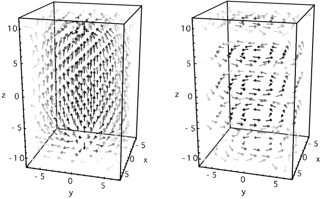
Figure 4: Profiles of electric field (left) and monopole current (right) at $\beta=2.5115$, with an Abelian Wilson loop of size 16$\times$4 on a $32^{4}$ lattice.

.

Before discussing the numerical simulation further, it is useful to consider what happens if we insert $W_{\mathit{Ph}}$ and $W_{\mathit{Mo}}$ into Eq. (23) instead of $W_{A}$. Using Eq. (5) and writing the Abelian field strength as $F=d\theta^{ph}+2\pi C^{(m)}\equiv F_{\mathit{Ph}}+F_{\mathit{Mo}}$, we can expect

$$\langle F\rangle_{j} = \frac{\langle(F_{\mathit{Ph}}+F_{\mathit{Mo}})W_{\mathit{Ph}}[j]W_{\mathit{Mo}}[j]\rangle_{0}}{\langle W_{\mathit{Ph}}[j]W_{\mathit{Mo}}[j]\rangle_{0}}\approx\frac{\langle F_{\mathit{Ph}}W_{\mathit{Ph}}[j]\rangle_{0}}{\langle W_{\mathit{Ph}}[j]\rangle_{0}}+\frac{\langle F_{\mathit{Mo}}W_{\mathit{Mo}}[j]\rangle_{0}}{\langle W_{\mathit{Mo}}[j]\rangle_{0}}=\langle F_{\mathit{Ph}}\rangle_{j}+\langle F_{\mathit{Mo}}\rangle_{j}\;.$$ (24)

Here, we have taken into account that in many cases lattice simulations in the MAG have found operators $X_{\mathit{Ph}}$ and $Y_{\mathit{Mo}}$, defined in terms of the photon part and the monopole part of the Abelian link variable $\theta$, respectively, to be uncorrelated: $\langle X_{\mathit{Ph}}Y_{\mathit{Mo}}\rangle_{0}\approx\langle X_{\mathit{Ph}}\rangle_{0}\langle Y_{\mathit{Mo}}\rangle_{0}$ (see, e.g., Ref. Bali:1996dm and references therein). From the relation (24), we expect that the sum of the flux profiles induced by the photon and monopole Wilson loops reproduces the total AP flux tube.

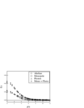
Figure 5: Electric field profile from correlators with Abelian, photon and monopole Wilson loops at $r=6a=0.48$ fm (left) and at $r=12a=0.97$ fm (right).

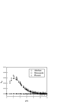
Figure 6: Monopole current profile from correlators with Abelian, photon and monopole Wilson loops at $r=6a=0.48$ fm (left) and at $r=12a=0.97$ fm (right).

Figure 7: The same plots as in Fig. 5, for flux tubes of length $r=0.48$ fm and $r=0.97$ fm, with the $E_{z}$ axis rescaled. The profile directly from the Abelian Wilson loop is omitted.

Second, let us consider the expectation value of the monopole current $k$. Since we have the obvious relation $k=-dC^{(m)}=k_{\mathit{Mo}}$, where a photon part of the monopole current does not exist, $k_{\mathit{Ph}}\propto d^{2}\theta^{ph}=0$, we will observe

$$\langle k\rangle_{j}\approx\frac{\langle k_{\mathit{Mo}}W_{\mathit{Mo}}[j]\rangle_{0}}{\langle W_{\mathit{Mo}}[j]\rangle_{0}}=\langle k_{\mathit{Mo}}\rangle_{j}.$$ (25)

This means that the correlator of the monopole current only with the monopole Wilson loop will account for the full expectation value of monopole current profile and, at the same time, the correlator with the photon Wilson loop vanishes everywhere.

We then show the corresponding lattice results, the electric field profile in Fig. 5 and the monopole current profile in Fig. 6, both as a function of the cylindrical radius. These measurements have been done at $\beta=2.5115$ on a $32^{4}$ lattice after the MAG has been fixed. The $q$-$\bar{q}$ distances are $r=6a$ and $12a$, and the measurements refer to the $x$-$y$ plane at half-distance. The lattice spacing is $a=0.081$ fm, which has been determined from the non-Abelian string tension $\sigma_{L}$, $\sqrt{\sigma_{phys}}=\sqrt{\sigma_{L}}/a\equiv 440$ MeV. Physically, the $q$-$\bar{q}$ distances correspond to 0.48 fm and 0.97 fm, respectively (see, Appendix B). In Fig. 7 we show the same electric field profiles as in Fig. 5, focussing on the region where the monopole part of $E_{z}$ becomes negative.

We find that these lattice results concerning the behavior of the profiles strongly support our considerations above; from the photon and the monopole Wilson loops, we obtain the Coulombic electric field and the solenoidal electric field with the monopole supercurrent profile, respectively. We find that the sum of these two contribution reproduces the profile obtained from the complete Abelian Wilson loop (see, Eq. (24)). There is no correlation between the photon Wilson loop and monopole current as anticipated in Eq. (25). Hence, we conclude that the AP flux tube has the same composed structure as the DAH flux tube.

The behavior of the profiles as a function of the $q$-$\bar{q}$ distance $r$ is also remarkable. While the monopole Wilson loop contributions, the solenoidal electric field and the monopole current profiles in the midplane are rather stable with respect to $r$, the photon Wilson loop contribution (i.e. the Coulombic electric field) drastically changes. From Fig. 5 it becomes obvious that the latter determines the change of the full Abelian electric field profile for different $r$. In order to see a really translationally invariant profile of the electric field, we need practically infinite $q$-$\bar{q}$ separation, $r\to\infty$. In this limit, the profile only from the monopole part remains. This situation is also the same in the DAH flux tube.

IV Summary

It has already been known that the profiles of the classical flux-tube solution in the dual Abelian Higgs (DAH) model and of the Abelian-projected (AP) flux tube, observed in lattice simulations in the maximally Abelian gauge (MAG), look quite similar.

In this paper, in order to establish a more detailed correspondence between these two kinds of profiles, we have studied the composed structure of both flux tubes more carefully. First, by applying the path-integral duality transformation to the Villain type compact QED considered as the approximate action of the AP gauge theory, we have been led to the U(1) DAH model. Along the way, we have identified the electric and magnetic parts of the Abelian Wilson loop by the Hodge decomposition, and have clarified the role of each contribution to the structure of the flux-tube solution in the DAH model. The photon and monopole Wilson loops provide sources of the Coulombic and solenoidal electric field components of the DAH flux tube.

Guided by this observation, we have performed lattice simulations of the SU(2) lattice gauge theory in the MAG and have measured the flux profiles induced by the photon and the monopole Wilson loops. We have found that the resulting profiles show the same composed structure as the DAH flux tube.

The further question would be how both sides are related quantitatively. One way would be to fit the profile of the AP flux tube by that of the DAH flux tube and to determine the DAH parameters which remain unknown in the formal derivation of the DAH model. Here, we would like to emphasize that the composed structure of the AP flux tube found here and its relation to the DAH flux tube will be important for further quantitative discussions. In fact, there is no such a work that takes into account the correspondence of the structures. In addition to this, as we have mentioned briefly in the introduction, a more systematic study of the AP flux-tube profile itself is required: the Gribov copy effect in the MAG, the scaling property, the $q$-$\bar{q}$ distance dependence, etc. Otherwise, one cannnot trust the robustness and physical relevance of the resulting DAH parameters. A part of such a quantitative analysis is reported in Lattice 2002 Koma:2002uq and the detailed report will be presented in Ref. koma-next .

In closing, we note that although we have concentrated here on SU(2) gauge theory, the ideas discussed in the present paper can be extended to arbitrary AP-SU($N$) gauge theory in the MAG Bornyakov:2001nd ; Koma:2002cv ; Ichie:2002mi .

Appendix A Classical flux-tube solution in the DAH model

In this appendix, we present concrete form of the field equations of the DAH model, Eqs. (19) and (20), for a straight $q$-$\bar{q}$ system. We use here the continuum notations; let $B^{mo}_{\mu}$ be the continuum form of the regular dual gauge field denoted $\tilde{\theta}_{\mu}^{mo}$ on the lattice, $B^{ph}_{\mu}$ that of the singular dual gauge field $\tilde{\theta}_{\mu}^{ph}$.

We put the quark and the antiquark at $\mbox{\boldmath$x$}_{1}=(-r/2)\mbox{\boldmath$e$}_{z}$ and $\mbox{\boldmath$x$}_{2}=(+r/2)\mbox{\boldmath$e$}_{z}$. The corresponding electric current is written as $j_{\mu}(x)=\delta_{\mu 0}\left(\delta(\mbox{\boldmath$x$}-\mbox{\boldmath$x$}_{1})-\delta(\mbox{\boldmath$x$}-\mbox{\boldmath$x$}_{2})\right)$. Since this system has cylindrical geometry, the fields can be parametrized in terms of cylindrical coordinates $(\rho,\varphi,z)$ as

$$\phi = \phi(\rho,z)\;,$$ (26)

$$\mbox{\boldmath$B$}^{mo} = B^{mo}(\rho,z)\mbox{\boldmath$e$}_{\varphi}\equiv\frac{\hat{B}^{mo}(\rho,z)}{\rho}\mbox{\boldmath$e$}_{\varphi}\;,$$ (27)

$$\mbox{\boldmath$B$}^{ph} = -\frac{n}{2\rho}\left(\frac{z+r/2}{\sqrt{\rho^{2}+(z+r/2)^{2}}}-\frac{z-r/2}{\sqrt{\rho^{2}+(z-r/2)^{2}}}\right)\mbox{\boldmath$e$}_{\varphi}\;.$$ (28)

The factor $n$ in $\mbox{\boldmath$B$}^{ph}$ is the winding number of the flux tube (an integer value), which is determined by the representation of the electric charges Koma:2001ut ; Koma:2001is ; Koma:2002cv . The fundamental representation corresponds to $n=1$.

The field equations (19) and (20) are then reduced to:

$$\beta_{m}\left(\frac{\partial^{2}\hat{B}^{mo}}{\partial\rho^{2}}-\frac{1}{\rho}\frac{\partial\hat{B}^{mo}}{\partial\rho}+\frac{\partial^{2}\hat{B}^{mo}}{\partial z^{2}}\right)$$

$$-2\left(\hat{B}^{mo}-\frac{n}{2}\left(\frac{z+r/2}{\sqrt{\rho^{2}+\left(z+r/2\right)^{2}}}-\frac{z-r/2}{\sqrt{\rho^{2}+\left(z-r/2\right)^{2}}}\right)\right)\phi^{2}=0,$$ (29)

$$\frac{\partial^{2}\phi}{\partial\rho^{2}}+\frac{1}{\rho}\frac{\partial\phi}{\partial\rho}+\frac{\partial^{2}\phi}{\partial z^{2}}$$

$$-\left(\frac{\hat{B}^{mo}-\frac{n}{2}\left(\frac{z+r/2}{\sqrt{\rho^{2}+\left(z+r/2\right)^{2}}}-\frac{z-r/2}{\sqrt{\rho^{2}+\left(z-r/2\right)^{2}}}\right)}{\rho}\right)^{2}\phi-2\lambda\phi(\phi^{2}-v^{2})=0.$$ (30)

The boundary conditions are specified so as to make the energy of the system finite as

$$\hat{B}^{mo}=0\quad{\rm as}\quad\rho\to 0,\quad{\rm and}\quad\phi=0\quad{\rm as}\quad\rho\to 0\quad{\rm for}\quad-r\leq z\leq r,$$

$$\hat{B}^{mo}=\frac{n}{2}\left(\frac{z+r/2}{\sqrt{\rho^{2}+\left(z+r/2\right)^{2}}}-\frac{z-r/2}{\sqrt{\rho^{2}+\left(z-r/2\right)^{2}}}\right)\quad{\rm and}\quad\phi=v\quad{\rm as}\quad\rho,\;z\to\infty\;.$$ (31)

After getting the numerical solution of the field equations for $\hat{B}^{mo}$ and $\phi$, the profiles of the electric field are computed as Eq. (21), where

$$\mbox{\boldmath$E$}^{mo} = -\frac{1}{\rho}\frac{\partial\hat{B}^{mo}}{\partial z}\mbox{\boldmath$e$}_{\rho}+\frac{1}{\rho}\frac{\partial\hat{B}^{mo}}{\partial\rho}\mbox{\boldmath$e$}_{z},$$ (32)

$$\mbox{\boldmath$E$}^{ph} = \frac{n}{2}\left(\frac{\rho}{(\rho^{2}+(z+r/2)^{2})^{3/2}}-\frac{\rho}{(\rho^{2}+(z-r/2)^{2})^{3/2}}\right)\mbox{\boldmath$e$}_{\rho}$$ (33)

$$+\frac{n}{2}\left(\frac{z+r/2}{(\rho^{2}+(z+r/2)^{2})^{3/2}}-\frac{z-r/2}{(\rho^{2}+(z-r/2)^{2})^{3/2}}\right)\mbox{\boldmath$e$}_{z}.$$

The profile of the monopole current (22) is given by

$$\mbox{\boldmath$k$}=2\left(\hat{B}^{mo}-\frac{n}{2}\left(\frac{z+r/2}{\sqrt{\rho^{2}+\left(z+r/2\right)^{2}}}-\frac{z-r/2}{\sqrt{\rho^{2}+\left(z-r/2\right)^{2}}}\right)\right)\phi^{2}\;\mbox{\boldmath$e$}_{\varphi}\;.$$ (34)

Appendix B lattice simulation detail

For the SU(2) link variables, $U_{\mu}(s)$, generated by Monte-Carlo method with Wilson gauge action, we adopt the maximally Abelian gauge (MAG) fixing, which is achieved by maximizing the functional

$$R[U^{V}]=\sum_{s,\mu}{\rm tr}\left\{\tau_{3}U^{V}_{\mu}(s)\tau_{3}U^{V~{}\dagger}_{\mu}(s)\right\}\;.$$ (35)

After the MAG fixing, Abelian projection is performed; the SU(2) link variables $U_{\mu}^{V}(s)=U_{\mu}^{MA}(s)$ are factorized into a diagonal (Abelian) link variable $u_{\mu}(s)\in{\rm U(1)}_{3}$ and the off-diagonal (charged matter field) parts $c_{\mu}(s)$, $c_{\mu}^{*}(s)\in{\rm SU(2)}/{\rm U(1)}_{3}$ as follows

$$U_{\mu}^{\mathit{MA}}(s)=\left(\begin{array}[]{cc}\sqrt{1-|c_{\mu}(s)|^{2}}&-c_{\mu}^{*}(s)\\ c_{\mu}^{*}(s)&\sqrt{1-|c_{\mu}(s)|^{2}}\end{array}\right)\left(\begin{array}[]{cc}u_{\mu}(s)&0\\ 0&u_{\mu}^{*}(s)\end{array}\right)\;,$$ (40)

where the Abelian link variables $u_{\mu}(s)$ are then explicitly written as

$$u_{\mu}(s)=e^{i\theta_{\mu}(s)}\quad(\theta_{\mu}(s)\in[-\pi,\pi))\;.$$ (41)

The Abelian plaquette variables is then constructed as

$$\theta_{\mu\nu}(s) \equiv \theta_{\mu}(s)+\theta_{\nu}(s+\hat{\mu})-\theta_{\mu}(s+\hat{\nu})-\theta_{\nu}(s)\quad\in[-4\pi,4\pi)\;,$$ (42)

which is decomposed into a regular part $\bar{\theta}_{\mu\nu}(s)\in[-\pi,\pi)$ and a singular (magnetic Dirac string) part $n_{\mu\nu}^{(m)}(s)=0,\pm 1,\pm 2$ as follows

$$\theta_{\mu\nu}(s) \equiv \bar{\theta}_{\mu\nu}(s)+2\pi n_{\mu\nu}^{(m)}(s)\;.$$ (43)

The Abelian field strength is defined by $\bar{\theta}_{\mu\nu}(s)=\theta_{\mu\nu}(s)-2\pi n_{\mu\nu}^{(m)}(s)$. Following DeGrand and Touissaint DeGrand:1980eq , magnetic monopoles are extracted as the string boundaries

$$k_{\mu}(s_{d})=-\frac{1}{2}\varepsilon_{\mu\nu\rho\sigma}\partial_{\nu}n_{\rho\sigma}^{(m)}(s+\hat{\mu})\qquad(\varepsilon_{1234}=1)\;,$$ (44)

where $|k_{\mu}(s_{d})|\leq 2$ and $s_{d}\equiv s+(\hat{1}+\hat{2}+\hat{3}+\hat{4})/2$ denotes the dual site.

For measuring the correlation function, we have used the following local operators: an electric field operator

$${\cal O}(s)=i\bar{\theta}_{i4}(s)=i(\theta_{i4}(s)-2\pi n_{i4}^{(m)}(s)),$$ (45)

and a monopole current operator

$${\cal O}(s_{d})=2\pi ik_{i}(s_{d})$$ (46)

The Abelian Wilson loop is constructed as

$$W_{A}[j]=\prod_{l\in j}u_{\mu}(s)=e^{i\sum_{l\in j}\theta_{\mu}(s)}.$$ (47)

Similarly, the photon and the monopole Wilson loop are constructed from the photon and monopole parts of Abelian link variables, $\theta^{ph}$ and $\theta^{mo}$, respectively, where

$$\theta_{\mu}(s)=\Delta^{-1}\partial_{\nu}(\bar{\theta}_{\mu\nu}(s)+2\pi n_{\mu\nu}^{(m)}(s))=\theta_{\mu}^{ph}(s)+\theta_{\mu}^{mo}(s).$$ (48)

In this decomposition, it is necessary to adopt the Abelian Landau gauge which is characterized by $\partial_{\mu}\theta_{\mu}(s)=0$. Note, however, that the Wilson loops constructed from each link variable are Abelian gauge invariant.

In this simulation, in order to see the profiles which belong to the ground state of a flux tube, we have adopted a smearing technique for spacelike Abelian link variables. Then we have constructed the smeared Abelian Wilson loop Bali:1996dm . Considering the fourth direction as the Euclidean time direction, we have performed $N_{s}$ times the following step in a smearing procedure applied only to the spatial Abelian links ($i,j=1,2,3$),

$$\alpha e^{i\theta_{i}(s)}+\sum_{j\neq i}e^{i(\theta_{j}(s)+\theta_{i}(s+\hat{j})-\theta_{j}(s+\hat{i}))}\to e^{i\theta_{i}(s)}\;,$$ (49)

where $\alpha$ is an appropriate smearing parameter. The same procedure was also applied to the spatial parts of the photon and the monopole link variables before constructing each type of Wilson loop.

The numerical simulations which are presented in this paper have been done at $\beta=$ 2.5115. The lattice volume was $32^{4}$. We have used 100 configurations for measurements. We have produced them after 3000 thermalization sweeps, separated by 500 Monte Carlo updates. They have been stored for performing MAG fixing. This has been repeated $N_{g}$ times, starting each time from a different random gauge copy of the configuration, in order to explore an increasing number of Gribov copies. The copy reaching the maximal value of the gauge functional (35) has been selected for measuring the profiles and kept for further increasing of $N_{g}$. Finally we have chosen $N_{g}=20$. For the MAG fixing itself, we have used the simulated annealing algorithm Bali:1996dm , followed by a final steepest descent relaxation. The size of the Wilson loops mainly studied (for Fig. 5, 6 and 7) are $R\times T$ = $6\times 6$ and $12\times 6$ in units of lattice spacing $a$. We have measured the profiles in the $x$-$y$ plane orthogonal to the Wilson loop in its midpoint. The Abelian smearing parameters have been found by optimization as $N_{s}=8$ and $\alpha=2.0$. With this choice, the profiles induced by the Abelian Wilson loop with timelike extensions $T=8$ and $T=6$ agree within errors.

The physical scale (the lattice spacing $a(\beta=2.5115)$) has been determined from the non-Abelian string tension $\sigma_{L}$ by fixing $\sqrt{\sigma_{phys}}=\sqrt{\sigma_{L}}/a\equiv 440$ MeV. The non-Abelian string tension has been re-evaluated by measuring expectation values of non-Abelian Wilson loops with an optimized non-Abelian smearing. The potential has been fitted to match the form $V(R)=C-A/R+\sigma_{L}\;R$. The resulting string tension is $\sigma_{L}=0.0323(4)$ at $\beta=2.5115$, such that the corresponding lattice spacing in physical units is $a(\beta)=0.0806(5)$ fm.

References

- (1) G. ’t Hooft, in High-Energy Physics. Proceedings of the EPS International Conference, Palermo, Italy, 23-28 June 1975, edited by A. Zichichi Vol. 2, pp. 1225–1249, Editrice Compositori, Bologna, 1976.
- (2) S. Mandelstam, Phys. Rept. 23C, 245 (1976).
- (3) A. A. Abrikosov, Sov. Phys. JETP 5, 1174 (1957).
- (4) H. B. Nielsen and P. Olesen, Nucl. Phys. B61, 45 (1973).
- (5) Y. Nambu, Phys. Rev. D10, 4262 (1974).
- (6) M. Creutz, QUARKS, GLUONS AND LATTICES (Cambridge, Uk: Univ. Pr. ( Cambridge Monographs On Mathematical Physics), 1983), 169p.
- (7) K. Sailer, T. Schoenfeld, Z. Schram, A. Schaefer, and W. Greiner, J. Phys. G17, 1005 (1991).
- (8) G. ’t Hooft, Nucl. Phys. B190, 455 (1981).
- (9) Z. F. Ezawa and A. Iwazaki, Phys. Rev. D25, 2681 (1982).
- (10) Z. F. Ezawa and A. Iwazaki, Phys. Rev. D26, 631 (1982).
- (11) T. Suzuki and I. Yotsuyanagi, Phys. Rev. D42, 4257 (1990).
- (12) D. Zwanziger, Phys. Rev. D3, 880 (1971).
- (13) K. Bardakci and S. Samuel, Phys. Rev. D18, 2849 (1978).
- (14) M. Stone and P. R. Thomas, Phys. Rev. Lett. 41, 351 (1978).
- (15) T. Suzuki, Prog. Theor. Phys. 80, 929 (1988).
- (16) S. Maedan and T. Suzuki, Prog. Theor. Phys. 81, 229 (1989).
- (17) H. Suganuma, S. Sasaki, and H. Toki, Nucl. Phys. B435, 207 (1995), hep-ph/9312350.
- (18) S. Sasaki, H. Suganuma, and H. Toki, Prog. Theor. Phys. 94, 373 (1995).
- (19) H. Shiba and T. Suzuki, Phys. Lett. B343, 315 (1995), hep-lat/9406010.
- (20) H. Shiba and T. Suzuki, Phys. Lett. B351, 519 (1995), hep-lat/9408004.
- (21) S. Kato, N. Nakamura, T. Suzuki, and S. Kitahara, Nucl. Phys. B520, 323 (1998).
- (22) M. N. Chernodub et al., Phys. Rev. D62, 094506 (2000), hep-lat/0006025.
- (23) T. Suzuki et al., Nucl. Phys. B (Proc. Suppl.) 106, 631 (2002), hep-lat/0110059.
- (24) V. Singh, D. A. Browne, and R. W. Haymaker, Phys. Lett. B306, 115 (1993), hep-lat/9301004.
- (25) Y. Matsubara, S. Ejiri, and T. Suzuki, Nucl. Phys. B (Proc. Suppl.) 34, 176 (1994), hep-lat/9311061.
- (26) P. Cea and L. Cosmai, Phys. Rev. D52, 5152 (1995), hep-lat/9504008.
- (27) G. S. Bali, C. Schlichter, and K. Schilling, Prog. Theor. Phys. Suppl. 131, 645 (1998), hep-lat/9802005.
- (28) S. Kamizawa, Y. Matsubara, H. Shiba, and T. Suzuki, Nucl. Phys. B389, 563 (1993).
- (29) Y. Koma, H. Suganuma, and H. Toki, Phys. Rev. D60, 074024 (1999), hep-ph/9902441.
- (30) Y. Koma, E.-M. Ilgenfritz, T. Suzuki, and H. Toki, Phys. Rev. D64, 014015 (2001), hep-ph/0011165.
- (31) E. T. Akhmedov, M. N. Chernodub, M. I. Polikarpov, and M. A. Zubkov, Phys. Rev. D53, 2087 (1996), hep-th/9505070.
- (32) D. Antonov and D. Ebert, Eur. Phys. J. C8, 343 (1999), hep-th/9806153.
- (33) D. Antonov and D. Ebert, Phys. Lett. B444, 208 (1998), hep-th/9809018.
- (34) M. N. Chernodub and D. A. Komarov, JETP Lett. 68, 117 (1998), hep-th/9809183.
- (35) Y. Koma, M. Koma, D. Ebert, and H. Toki, JHEP 08, 047 (2002), hep-th/0108138.
- (36) Y. Koma, M. Koma, D. Ebert, and H. Toki, Nucl. Phys. B648, 189 (2003), hep-th/0206074.
- (37) F. V. Gubarev, E.-M. Ilgenfritz, M. I. Polikarpov, and T. Suzuki, Phys. Lett. B468, 134 (1999), hep-lat/9909099.
- (38) J. D. Stack, S. D. Neiman, and R. J. Wensley, Phys. Rev. D50, 3399 (1994), hep-lat/9404014.
- (39) H. Shiba and T. Suzuki, Phys. Lett. B333, 461 (1994), hep-lat/9404015.
- (40) G. S. Bali, V. Bornyakov, M. Mueller-Preussker, and K. Schilling, Phys. Rev. D54, 2863 (1996), hep-lat/9603012.
- (41) Y. Koma, M. Koma, E.-M. Ilgenfritz, and T. Suzuki, A detailed study of the Abelian-projected SU(2) flux tube and its dual Ginzburg-Landau analysis, 2003, hep-lat/0308008.
- (42) M. N. Chernodub and M. I. Polikarpov, Abelian projections and monopoles, 1997, hep-th/9710205.
- (43) T. Suzuki and M. N. Chernodub, Screening and confinement in Abelian effective theories, 2002, hep-lat/0207018.
- (44) T. Banks, R. Myerson, and J. Kogut, Nucl. Phys. B129, 493 (1977).
- (45) M. E. Peskin, Ann. Phys. 113, 122 (1978).
- (46) Y. Koma, M. Koma, T. Suzuki, E.-M. Ilgenfritz, and M. I. Polikarpov, Nucl. Phys. B (Proc. Suppl.) 119, 676 (2003), hep-lat/0210014.
- (47) V. Bornyakov et al., Nucl. Phys. B (Proc. Suppl.) 106, 634 (2002), hep-lat/0111042.
- (48) Y. Koma, Phys. Rev. D66, 114006 (2002), hep-ph/0208066.
- (49) H. Ichie, V. Bornyakov, T. Streuer, and G. Schierholz, (2002), hep-lat/0212024.
- (50) Y. Koma, E.-M. Ilgenfritz, H. Toki, and T. Suzuki, Phys. Rev. D64, 011501 (2001), hep-ph/0103162.
- (51) Y. Koma and M. Koma, Eur. Phys. J. C26, 457 (2003), hep-ph/0109033.
- (52) T. A. DeGrand and D. Toussaint, Phys. Rev. D22, 2478 (1980).