Lattice QCD at non-vanishing density: phase diagram, equation of state

Abstract

We propose a method to study lattice QCD at non-vanishing temperature ($T$) and chemical potential ($\mu$). We use $n_{f}$=2+1 dynamical staggered quarks with semi-realistic masses on $L_{t}$=4 lattices. The critical endpoint (E) of QCD on the Re($\mu$)-T plane is located. We calculate the pressure (p), the energy density ($\epsilon$) and the baryon density ($n_{B}$) of QCD at non-vanishing T and $\mu$.

1 Introduction

QCD at finite $T$ and/or $\mu$ is of fundamental importance, since it describes physics relevant in the early universe, in neutron stars and in heavy ion collisions. Extensive experimental work has been done with heavy ion collisions at CERN and Brookhaven to explore the $\mu$-$T$ phase boundary (cf. [1]). Note, that past, present and future heavy ion experiments with always higher and higher energies produce states closer and closer to the $T$ axis of the $\mu$-$T$ diagram. It is a long-standing question, whether a critical point exists on the $\mu$-$T$ plane, and particularly how to tell its location theoretically [2].

Universal arguments [3] and lattice results [4] indicate that at $\mu$=0 the real world probably has a crossover. Arguments based on a variety of models (see e.g. [6, 7, 2]) predict a first order finite $T$ phase transition at large $\mu$. Combining the $\mu=0$ and large $\mu$ informations suggests that the phase diagram features a critical endpoint $E$ (with chemical potential $\mu_{E}$ and temperature $T_{E}$), at which the line of first order phase transitions ($\mu>\mu_{E}$ and $T<T_{E}$) ends [2]. At E the phase transition is of second order and long wavelength fluctuations appear, which results in (see e.g. [8]) consequences, similar to critical opalescence. Passing close enough to ($\mu_{E}$,$T_{E}$) one expects simultaneous signatures which exhibit non-monotonic dependence on the control parameters [9], since one can miss the critical point on either side.

The location of E is an unambiguous, non-perturbative prediction of QCD. No ab initio, lattice QCD study based was done to locate E. Crude models with $m_{s}=\infty$ were used (e.g. [2]) suggesting that $\mu_{E}\approx$ 700 MeV, which should be smaller for finite $m_{s}$. The goal of our work is to propose a new method to study lattice QCD at finite $\mu$ and apply it to locate the endpoint. We use full QCD with dynamical $n_{f}$=2+1 staggered quarks.

QCD at finite $\mu$ can be given on the lattice [10]; however, standard Monte-Carlo techniques fail. At Re($\mu$)$\neq$0 the determinant of the Euclidean Dirac operator is complex, which spoils any importance sampling method.

Several suggestions were studied in detail to solve the problem.

For small gauge coupling an attractive approach is the “Glasgow method” [11] in which the partition function is expanded in powers of $\exp(\mu/T)$ by using an ensemble of configurations weighted by the $\mu$=0 action. After collecting more than 20 million configurations only unphysical results were obtained: a premature onset transition. The reason is that the $\mu$=0 ensemble does not overlap sufficiently with the states of interest. We show how to handle this problem for small $\mu$ values.

At imaginary $\mu$ the measure remains positive and standard Monte Carlo techniques apply. One can also use the fact that the partition function away from the transition line should be an analytic function of $\mu$, and the fit for imaginary $\mu$ values could be analytically continued to real values of $\mu$ [12, 13].

Due to the renewed interest several promising ideas appeared in the last years (without giving a complete list see e.g. [14, 15, 16, 17, 18]).

Figure 1: Schematic difference between the present and the Glasgow methods.

We propose a method to reduce the overlap problem and determine the phase diagram in the $\mu$-T plane (for details see [19]). The idea is to produce an ensemble of QCD configurations at $\mu$=0 and at the transition temperature $T_{c}$. Then we determine the Boltzmann weights [20] of these configurations at $\mu\neq 0$ and at $T$ lowered to the transition temperatures at this non-vanishing $\mu$. Since transition configurations are reweighted to transition ones a much better overlap can be observed than by reweighting pure hadronic configurations to transition ones [11]. Since the original ensemble is collected at $\mu$=0 we do not expect it to be able to describe the physics of the large $\mu$ region with e.g. exotic colour superconductivity. Fortunately, the typical $\mu$ values at present heavy ion accelerators are smaller than the region we cover.

We illustrate the applicability of the method and locate the critical point of QCD. (Multi-dimensional reweighting was successful for determining the endpoint of the hot electroweak plasma [22] e.g. on 4D lattices.) Furthermore we give the equation of state of the QCD plasma at non-vanishing temperature and chemical potential.

2 Overlap improving multi-parameter reweighting

Let us study a generic system of fermions $\psi$ and bosons $\phi$, where the fermion Lagrange density is ${\bar{\psi}}M(\phi)\psi$. Integrating over the Grassmann fields we get:

$$Z(\alpha)=\int{D}\phi\exp[-S_{bos}(\alpha,\phi)]\det M(\phi,\alpha),$$ (1)

where $\alpha$ is the parameter set of the Lagrangian. In the case of staggered QCD $\alpha$ consists of $\beta$, $m_{q}$ and $\mu$. For some choice of the parameters $\alpha$=$\alpha_{0}$ importance sampling can be done (e.g. for Re($\mu$)=0). Rewriting eq. (1)

$$Z(\alpha)=\int{D}\phi\exp[-S_{bos}(\alpha_{0},\phi)]\det M(\phi,\alpha_{0})$$

$$\left\{\exp[-S_{bos}(\alpha,\phi)+S_{bos}(\alpha_{0},\phi)]{\det M(\phi,\alpha)\over\det M(\phi,\alpha_{0})}\right\}.$$ (2)

The curly bracket is measured on each independent configuration and is interpreted as a weight factor $\{w(\beta,\mu,m,U)\}$. The rest is treated as the integration measure. Changing only one parameter of the ensemble generated at $\alpha_{0}$ provides an accurate value for some observables only for high statistics. This is ensured by rare fluctuations as the mismatched measure occasionally sampled the regions where the integrand is large. This is the overlap problem. Having several parameters the set $\alpha_{0}$ can be adjusted to get a better overlap than obtained by varying only one parameter.

The basic idea of the method as applied to dynamical QCD can be summarized as follows. We study the system at ${\rm Re}(\mu)$=0 around its transition point. Using a Glasgow-type technique we calculate the determinants for each configuration for a set of $\mu$, which, similarly to the Ferrenberg-Swendsen method [20], can be used for reweighting. The average plaquette values can be used to perform an additional reweighting in $\beta$. Since transition configurations were reweighted to transition ones a much better overlap can be observed than by reweighting pure hadronic configurations to transition ones as done by the Glasgow-type techniques. The differences between the two methods are shown in Figure 1. (Note, that reweighting techniques have very broad applicability. E.g. recently it was possible to determine the topological susceptibility with overlap fermions [21].)

3 The endpoint of $n_{f}=2+1$ QCD

In QCD with $n_{f}$ staggered quarks one changes the determinants to their $n_{f}$/4 power in our two equations. Importance sampling works at some $\beta$ and at Re($\mu$)=0. Since $\det M$ is complex an additional problem arises, one should choose among the possible Riemann-sheets of the fractional power in eq. (2). This can be done by using [19] the fact that at $\mu$=$\mu_{w}$ the ratio of the determinants is 1 and it should be a continuous function of $\mu$.

In the following we keep $\mu$ real and look for the zeros of $Z$ for complex $\beta$. At a first order phase transition the free energy $\propto\log Z(\beta)$ is non-analytic. A phase transition appears only in the V$\rightarrow\infty$ limit, but not in a finite $V$. Nevertheless, $Z$ has zeros at finite V, which are at complex parameters (e.g. $\beta$). For a system with first order transition these zeros approach the real axis as V$\rightarrow\infty$ by a $1/V$ scaling. This V$\rightarrow\infty$ limit generates the non-analyticity of the free energy. For a system with crossover $Z$ is analytic, and the zeros do not approach the real axis as V$\rightarrow\infty$.

Figure 2: The T-$\mu$ diagram. Direct results are given with errorbars. The dotted line shows the crossover, the solid line the first order transition. The box gives the uncertainties of the endpoint.

At T$\neq$0 we used $L_{t}$=4, $L_{s}$=4,6,8 lattices. T=0 runs were done on $10^{3}\cdot$ 16 lattices. $m_{u,d}$=0.025 and $m_{s}$=0.2 were our bare quark masses. At $T\neq 0$ we determined the complex valued Lee-Yang zeros [23], $\beta_{0}$, for different V-s as a function of $\mu$. Their V$\rightarrow\infty$ limit was given by a $\beta_{0}(V)=\beta_{0}^{\infty}+\zeta/V$ extrapolation. We used 14000, 3600 and 840 configurations on $L_{s}$=4,6 and $8$ lattices, respectively. For small $\mu$ values Im($\beta_{0}^{\infty}$) is inconsistent with zero, and predicts a crossover. Increasing $\mu$, the value of Im($\beta_{0}^{\infty}$) decreases. Thus the transition becomes consistent with a first order phase transition. Our primary result is $\mu_{end}=0.375(20)$ in lattice units.

To set the physical scale we used an average of $R_{0}$, $m_{\rho}$ and $\sqrt{\sigma}$. Including systematics due to finite V we have $(R_{0}\cdot m_{\pi})=0.73(6)$, which is at least twice, $m_{u,d}$ is at least four times as large as the physical values.

Figure 2 shows the phase diagram in physical units, thus $T$ as a function of $\mu_{B}$, the baryonic chemical potential (which is three times larger than the quark chemical potential). The endpoint is at $T_{E}=160\pm 3.5$ MeV, $\mu_{E}=725\pm 35$ MeV. At $\mu_{B}$=0 we obtained $T_{c}=172\pm 3$ MeV.

Using a Taylor expansion around $\mu$=0, T$\neq$0 for small $\mu$ can be used to determine the curvature of the phase diagram and to calculate thermal properties [24]. A different method, analytic continuation from imaginary $\mu$, confirmed also the results of [19] on the $\mu$–$T$ diagram [12, 13].

4 Equation of state at non-vanishing T and $\mu$

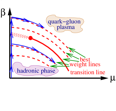
Figure 3: The best weight lines on the $\mu$–$\beta$ plane. In the middle we indicate the transition line. Its first dotted part is the crossover region. The blob represents the critical endpoint, after which the transition is of first order. The integration paths used to calculate $p$ are shown by the arrows along the $\beta$ axis and the best weight lines.

The equation of state (EOS) at $\mu$$\neq$0 is essential to describe the quark gluon plasma (QGP) formation at heavy ion collider experiments. Results are only available for $\mu$=0 (e.g. [25, 26, 27]) at T$\neq$0.

Figure 4: $p$ normalised by $T^{4}$ as a function of $T/T_{c}$ at $\mu=0$ (to help the continuum interpretation the raw lattice result is multiplied by $c_{\mu}$=0.446).

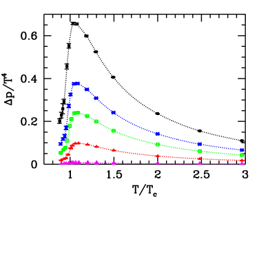
Figure 5: $\Delta p=p(\mu\neq 0,T)-p(\mu=0,T)$ normalised by $T^{4}$ as a function of $T/T_{c}$ for $\mu_{B}$=100, 210, 330, 410 MeV and 530 MeV (from bottom to top). To help the continuum interpretation the raw lattice result is multiplied by $c_{\mu}$=0.446.

We use 4 $\cdot N_{s}^{3}$ lattices at $T$$\neq$0 with $N_{s}$=8,10,12 for reweighting and we extrapolate to V$\rightarrow$$\infty$ using the available volumes ($V$). At $T$=0 lattices of $24\cdot 14^{3}$ are taken for vacuum subtraction and to connect lattice parameters to physical quantities. 14 different $\beta$ values are used, which correspond to $T/T_{c}=0.8,\dots,3$. Our T=0 simulations provided $R_{0}$ and $\sigma$. The lattice spacing at $T_{c}$ is $\approx$0.25–0.30 fm. We use 2+1 flavours of dynamical staggered quarks. While varying $\beta$ (thus T) we keep the physical quark masses approx. constant (the pion to rho mass ratio is $m_{\pi}/m_{\rho}\approx$0.66).

The determination of the equation of state at $\mu\neq$0 needs several observables, ${O}$, at $\mu$$\neq$0. This is obtained by using the weights of eq. (2)

$${\overline{O}}(\beta,\mu,m)=\frac{\sum\{w(\beta,\mu,m,U)\}{O}(\beta,\mu,m,U)}{\sum\{w(\beta,\mu,m,U)\}}.$$ (3)

$p$ can be obtained from the partition function as $p$=$T\cdot\partial\log Z/\partial V$ which can be written as $p$=(T/V)$\cdot\log Z$ for large homogeneous systems. On the lattice we can only determine the derivatives of $\log Z$ with respect to the parameters of the action ($\beta,m,\mu$). Using the notation $\langle{O}(\beta,\mu,m)\rangle$= ${\overline{{{O}}}(\beta,\mu,m)}_{T\neq 0}-{\overline{{O}}(\beta,\mu=0,m)}_{T=0}$. $p$ can be written as an integral [28]:

$$\frac{p}{T^{4}}=\frac{1}{T^{3}V}\int d(\beta,m,\mu)$$ (4)

$$\left(\left\langle\frac{\partial(\log Z)}{\partial\beta}\right\rangle,\left\langle\frac{\partial(\log Z)}{\partial m}\right\rangle,\left\langle\frac{\partial(\log Z)}{\partial\mu}\right\rangle\right).$$

The integral is by definition independent of the integration path. The chosen integration paths are shown in Fig 3.

The energy density can be written as $\epsilon=(T^{2}/V)\cdot\partial(\log Z)/\partial{T}+(\mu T/V)\cdot\partial(\log Z)/\partial\mu$. By changing the lattice spacing $T$ and $V$ are simultaneously varied. The special combination $\epsilon-3p$ contains only derivatives with respect to $a$ and $\mu$:

$$\frac{\epsilon-3p}{T^{4}}=-\left.\frac{a}{T^{3}V}\frac{\partial\log(Z)}{\partial a}\right|_{\mu}+\left.\frac{\mu}{T^{3}V}\frac{\partial(\log Z)}{\partial\mu}\right|_{a}.$$ (5)

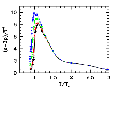
Figure 6: $(\epsilon-3p)/T^{4}$ at $\mu_{B}$=0, 210, 410 MeV and 530 MeV versus $T/T_{c}$ (from bottom to top). To help the continuum interpretation the raw lattice result is multiplied by $c_{p}$=0.518.

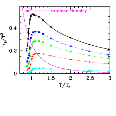
Figure 7: $n_{B}/T^{3}$ versus $T/T_{c}$ for the same $\mu_{B}$ values as in Fig. 3 (from bottom to top). (to help the continuum interpretation the raw lattice result is multiplied by $c_{\mu}$=0.446). As a reference value the line starting in the left upper corner indicates the nuclear density.

The quark number density is $n=(T/V)\cdot\partial\log(Z)/\partial\mu$ which can be measured directly or obtained from $p$ (baryon density is $n_{B}$=$n$/3 and baryonic chemical potential is $\mu_{B}$=3$\mu$).

We present direct lattice results on $p(\mu=0,T)$, $\Delta p(\mu,T)=p(\mu\neq 0,T)-p(\mu=0,T)$, $\epsilon(\mu,T)$-3$p(\mu,T)$ and $n_{B}(\mu,T)$. Additional overall factors were used to help the phenomenological interpretation.

Fig. 4 shows $p$ at $\mu$=0. In Fig. 5 we show $\Delta p/T^{4}$ for different $\mu$ values. Fig. 6 shows $\epsilon$-3$p$ normalised by $T^{4}$, which tends to zero for large $T$. Fig. 7 gives the baryonic density as a function of $T/T_{c}$ for different $\mu$-s. The densities can exceed the nuclear density by up to an order of magnitude.

An important finding concerns the applicability of our reweighting method: the maximal $\mu$ scales with the volume as $\mu_{\rm{max}}\cdot a\sim(N_{t}\cdot N_{s}^{3})^{-0.25}$. If this behaviour persists, one could –in principle– approach the true continuum limit ($a\sim 1/N_{t}\sim(N_{t}\cdot N_{s}^{3})^{-0.25}$, thus $\mu_{\rm{max}}$$\approx$const.).

5 Conclusion

We proposed a method –an overlap improving multi-parameter reweighting technique– to numerically study non-zero $\mu$ and determine the phase diagram in the $T$-$\mu$ plane. Our method is applicable to any number of Wilson or staggered quarks.

We studied the $\mu$-$T$ phase diagram of QCD with dynamical $n_{f}$=2+1 quarks. Using our method we obtained $T_{E}$$\approx$160 MeV and $\mu_{E}$$\approx$700 MeV for the endpoint. Though $\mu_{E}$ is too large to be studied at RHIC or LHC, the endpoint would probably move closer to the $\mu$=0 axis when the quark masses get reduced.

The equation of state was determined on the temperature versus chemical potential plane. According to our results the applicability range of the overlap improving multi-parameter reweighting method for the quark chemical potential can be summarized as $\mu\mathop{\raise 1.29167pt\hbox{$<$\kern-7.5pt\raise-4.73611pt\hbox{$\sim$}}}T$.

Clearly, more work is needed to get the final values by extrapolating in the R-algorithm and to the thermodynamic, chiral and continuum limits. The details of the presented results can be found in [19, 29].

References

- [1] J. Stachel, these proceedings.
- [2] M. Halasz et al. Phys. Rev. D58 (1998) 096007; J. Berges, K. Rajagopal, Nucl. Phys. B538 (1999) 215. M. Stephanov, K. Rajagopal, E. Shuryak, Phys. Rev. Lett. 81 (1998) 4816; T.M. Schwarz, S.P. Klevansky, G. Papp, Phys. Rev. C60 (1999) 055205.
- [3] R. Pisarski and F. Wilczek, Phys. Rev. D29 (1984) 338; F. Wilczek, Int. J. Mod. Phys. A7 (1992) 3911; K. Rajagopal and F. Wilczek, Nucl. Phys. B399 (1993) 395.
- [4] For recent reviews see: A. Ukawa, Nucl. Phys. Proc. Suppl. 53 (1997) 106; E. Laerman, ibid. 63 (1998) 114; F. Karsch, ibid. 83 (2000) 14; S. Ejiri, ibid. 94 (2001) 19; S. Hands, ibid 106 (2002) 142; J. B. Kogut, arXiv:hep-lat/0208077; a review comparing recent analytic and lattice results: M. G. Alford, arXiv:hep-ph/0209287.
- [5] F.K. Brown, Phys. Rev. Lett. 65 (1990) 2491; S. Aoki et al., Nucl. Phys. Proc. Suppl. 73 (1999) 459.
- [6] A. Barducci et al., Phys. Lett. B231 (1989) 463; Phys. Rev. D41 (1990) 1610; ibid. D49 (1994) 426; S.P. Klevansky, Rev. Mod. Phys. 64 (1992) 649; M. Stephanov, Phys. Rev. Lett. 76, (1996) 4472.
- [7] M. Alford, K. Rajagopal and F. Wilczek, Phys. Lett. B422 (1998) 247; Nucl. Phys. B537 (1999) 443; R. Rapp, T. Schäfer, E.V. Shuryak and M. Velkovsky, Phys. Rev. Lett. 81 (1998) 53; for a recent review with references see K. Rajagopal and F. Wilczek, hep-ph/0011333.
- [8] S. Borsányi et al., Phys. Rev. D64 (2001) 125011.
- [9] M. Stephanov, K. Rajagopal and E. Shuryak, Phys. Rev. D60 (1999) 114028.
- [10] P. Hasenfratz and F. Karsch, Phys. Lett. B125 (1983) 308; J. Kogut et al., Nucl. Phys. B225 (1983) 93.
- [11] I.M. Barbour et al., Nucl. Phys. B (Proc. Suppl.) 60A (1998) 220.
- [12] P. de Forcrand and O. Philipsen, hep-lat/0205016; hep-lat/0209084; P. de Forcrand, these proceedings.
- [13] M. D’Elia, M.P. Lombardo, hep-lat/0209146.
- [14] D. K. Hong and S. D. Hsu, Phys. Rev. D 66 (2002) 071501; D. K. Hong, these proceedings arXiv:hep-ph/0301125.
- [15] J. Ambjorn et al., JHEP 0210 (2002) 062
- [16] U. J. Wiese, Nucl. Phys. A 702 (2002) 211.
- [17] K. F. Liu, Int. J. Mod. Phys. B 16 (2002) 2017.
- [18] G. Akemann and T. Wettig, these proceedings, arXiv:hep-lat/0301017.
- [19] Z. Fodor, S. D. Katz, Phys. Lett. B 534 (2002) 87; JHEP 0203 (2002) 014.
- [20] A.M. Ferrenberg, R.H. Swendsen, Phys. Rev. Lett. 63 (1989) 1195; 61 (1988) 2635.
- [21] T. G. Kovacs, arXiv:hep-lat/0111021.
- [22] Y. Aoki et al., Phys. Rev. D60 (1999) 013001; F. Csikor, Z. Fodor and J. Heitger, Phys. Rev. Lett. 82 (1999) 21; for details of the electroweak simulations see e.g. F. Csikor et al., Phys. Lett. B 357 (1995) 156 and references therein.
- [23] C.N. Yang and T.D. Lee, Phys. Rev. 87 (1952) 404.
- [24] C. R. Allton et al., hep-lat/0204010; S. Ejiri et al., hep-lat/0209012; C. Schmidt et al, hep-lat/0209009, C. Schmidt, hep-lat/0210037, S. Ejiri, hep-lat/0212022.
- [25] S. Gottlieb et al., Phys. Rev. D 55 (1997) 6852.
- [26] F. Karsch, E. Laermann and A. Peikert, Phys. Lett. B 478 (2000) 447.
- [27] A. Ali Khan et al. [CP-PACS collaboration], Phys. Rev. D 64 (2001) 074510.
- [28] J. Engels et al., Phys. Lett. B 252 (1990) 625.
- [29] Z. Fodor, S.D. Katz and K.K. Szabó, hep-lat/0208078; F. Csikor et al., in preparation.