Matrix model correlation functions and lattice data for the QCD Dirac operator with chemical potential

Abstract

We apply a complex chiral random matrix model as an effective model to QCD with a small chemical potential at zero temperature. In our model the correlation functions of complex eigenvalues can be determined analytically in two different limits, at weak and strong non-Hermiticity. We compare them to the distribution of the smallest Dirac operator eigenvalues from quenched QCD lattice data for small values of the chemical potential, appropriately rescaled with the volume. This confirms the existence of two different scaling regimes from lattice data.

1 Introduction

The presence of a chemical potential $\mu$ in QCD remains a challenging problem, due to the fact that the Dirac operator eigenvalues become complex. One possibility to study this situation analytically is given by random matrix models. The origin of such an effective description for real Dirac eigenvalues at $\mu=0$, as first suggested in [Jac], is by now very well established, and we refer to [JT] for a review. A chiral random matrix model including a chemical potential was proposed in [Steph]. While its partition function and susceptibilities were determined analytically in [Halasz], the microscopic correlation functions are not known to date. Very recently the model has been simulated on the lattice [Kostas], confirming the results of [Halasz]. In [MPW] complex Dirac spectra have been analyzed using quenched lattice data in the bulk of the spectrum. Here chiral symmetry is not important, and the relevant matrix model correlations are given by the known results for the Ginibre ensemble [Gin]. A transition starting from the Gaussian unitary ensemble (GUE) at $\mu=0$ via the Ginibre to the Poisson ensemble was observed [MPW].

Very recently an alternative chiral matrix model with complex eigenvalues was introduced and solved in [A02]. Here the microscopic, complex correlation functions are calculated in two different limits. The first limit is called weakly non-Hermitian and was discovered in [FKS]. It interpolates between the chiral GUE [Jac] and the correlations in the second limit at strong non-Hermiticity. The results of Ginibre [Gin] are at strong non-Hermiticity, too, but differ from [A02] due to chiral symmetry. We note that the model [A02] is always in the phase with broken chiral symmetry, in contrast to [Steph].

2 Chiral random matrix theory with complex eigenvalues

In this section we summarize the results of the complex extension [A02] of the chiral GUE. The matrix model partition function is defined as

$$Z^{(a)}(\tau) \equiv \int\limits_{\mathbb{C}^{N}}\prod_{j=1}^{N}dz_{j}^{2}\ |z_{j}|^{2a+1}\exp\!\left[-\frac{N}{1-\tau^{2}}\left(|z_{j}|^{2}-\frac{\tau}{2}(z_{j}^{2}+z_{j}^{\ast\,2})\right)\right]$$ (1)

$$\times\prod_{k>l}^{N}\left|z_{k}^{2}-z_{l}^{2}\right|^{2}.$$

In analogy to the chiral GUE [Jac], the power $a=N_{f}+\nu$ combines the number of massless quark flavors $N_{f}$ and the topological charge $\nu$. The non-Hermiticity parameter $\tau\in[0,1]$ relates to the chemical potential $\mu$ via

$$4\mu^{2}\ =\ 1-\tau^{2}$$ (2)

from comparing [Steph] and [A02] at small $\mu$. For $\tau\to 1$, the complex eigenvalues $z_{j}$ become real, and we recover the partition function of the chiral GUE [Jac]. In the limit $\tau\to 0$, the non-Hermiticity is maximal, and eq. (1) becomes a chiral extension of the Ginibre ensemble [Gin]. The relation between the matrix model [Steph] and eq. (1) consists in a nontrivial mapping of the complex phase of the Dirac determinant in the former to the exponent of the latter, and we conjecture that the two models are in the same universality class.

The model of eq. (1) is solved at finite and large $N$ using the technique of orthogonal polynomials in the complex plane [A02]. We distinguish two different large-$N$ limits: in the weakly non-Hermitian limit [FKS] we keep

$$\lim_{N\to\infty}\lim_{\tau\to 1}\ N(1-\tau^{2})\equiv\alpha^{2}$$ (3)

fixed. We thus send $\mu\to 0$ such that the volume $V$ times $\mu^{2}$ is fixed. In this limit the eigenvalues macroscopically collapse to the real line while microscopically they still extend into the complex plane. At strong non-Hermiticity we take $N\to\infty$ at fixed $\tau\in[0,1)$. In this limit the macroscopic eigenvalue density becomes constant on an ellipse in the complex plane.

The result for the microscopic density at weak non-Hermiticity reads

$$\rho^{(a)}_{\rm weak}(\xi)=\frac{\sqrt{\pi\alpha^{2}}}{\mbox{erf}(\alpha)}\ |\xi|\ \exp\!\left[\frac{-1}{\alpha^{2}}(\Im m\,\xi)^{2}\right]\int_{0}^{1}dt\ \mbox{e}^{-\alpha^{2}t}J_{a}(\sqrt{t}\xi)J_{a}(\sqrt{t}\xi^{\ast})\>,$$ (4)

where we have rescaled the complex eigenvalues $\xi\equiv Nz\sqrt{2}$ with the same power in $N$ as for real eigenvalues [Jac]. In contrast, we obtain for the microscopic density at strong non-Hermiticity${}^{\mbox{\scriptsize a}}$

$$\rho^{(a)}_{\rm strong}(\xi)=\sqrt{\frac{\pi}{1-\tau^{2}}}\ |\xi|\ \exp\!\left[\frac{-1}{2(1-\tau^{2})}\,|\xi|^{2}\right]I_{a}\left(\frac{|\xi|^{2}}{2(1-\tau^{2})}\right),$$ (5)

rescaling $\xi\equiv\sqrt{2N}\,z$ here. For the higher order $k$-point eigenvalue correlation functions in both limits we refer to [A02].

3 Comparison with lattice data

In this section we compare quenched QCD lattice data with the predictions of eqs. (4) and (5). The data were generated on a $6^{4}$ lattice at gauge coupling $\beta=5.0$ using staggered fermions. We have chosen two different values for the chemical potential, $\mu=0.006$ and $\mu=0.2$, with 3500 and 4500 configurations, respectively, corresponding to the two different regimes of weak and strong non-Hermiticity. In both cases, we are concentrating on the microscopic scale (i.e. a few eigenvalues) so that instead of unfolding the data we only need to rescale them by the mean level spacing.

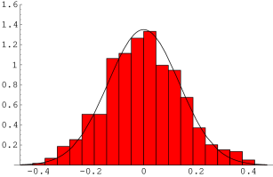
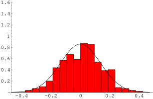
Figure 1: Cuts of the Dirac eigenvalue density for fixed real part of the eigenvalues, plotted vs the imaginary part, for $\mu=0.006$, along with eq. (4). Left: real part corresponds to first maximum in Fig. 2, right: real part corresponds to first minimum in Fig. 2.

For $\mu=0.006$ we determine the parameter $\alpha$ from the weak limit by a fit to the decay into the complex plane for a fixed real value, as shown in Fig. 1.

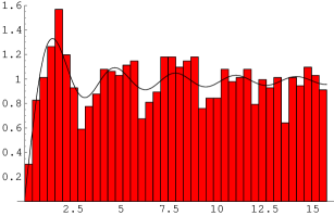
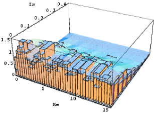
Figure 2: Left: cut of the Dirac eigenvalue density along the real axis for $\mu=0.006$, along with eq. (4). Right: the density in the complex plane, along with eq. (4) (which is slightly displaced for comparison).

We find on average $\alpha=0.19$, varying about 4% when determined along the first maximum or minimum on the real axis. This agrees roughly with $\alpha\sim 0.27$ obtained from eqs. (2, 3) and the rescaled level spacing. The discrepancy may be due to the uncertainty in the latter and will be further investigated. In Fig. 2 (left) we show a section of the data along the real axis. Since $\alpha$ is small, we could equally well plot the real density [Jac], $\rho^{(a)}_{\rm real}(\xi)=\frac{1}{2}\pi\xi[J_{0}(\xi)^{2}+J_{1}(\xi)^{2}]$, differing by $\leq 0.5\%$. The histogram in Fig. 2 (right) shows the quantitative agreement in the complex plane.

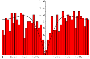
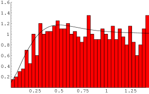
Figure 3: Cuts of the Dirac eigenvalue density for $\mu=0.2$, along with eq. (5). Left: cut along the imaginary axis, right: cut along the real axis.

At strong non-Hermiticity we rescale the data for $\mu=0.2$ independently in the real and imaginary directions with the square root of the respective level spacing. Cuts along the axes are shown in Fig. 3, and the complete plot is in Fig 4. Here we have used the relation (2) instead of fitting, leading to $\tau=0.9165$. The repulsion of the eigenvalues from the origin, which is very different from that in the weak limit, is clearly seen in the data.

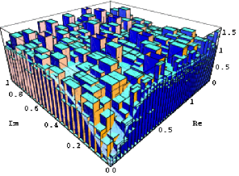
Figure 4: Dirac eigenvalue density and eq. (5) in the complex plane for $\mu=0.2$.

4 Conclusions

In this first exploratory study, we found good agreement between the predictions of the model (1) and data from lattice QCD simulations. In particular, the two predicted scaling regimes corresponding to weak and strong non-Hermiticity are clearly visible in the data. Obviously, more work is needed to make these conclusions more quantitative (e.g. larger volume, higher statistics, unfolding details).

References

- [1] E.V. Shuryak and J.J.M. Verbaarschot, Nucl. Phys. A560, 306 (1993); J.J.M. Verbaarschot, Phys. Rev. Lett. 72, 2531 (1994).
- [2] J.J.M. Verbaarschot and T. Wettig, Ann. Rev. Nucl. Part. Sci. 50, 343 (2000).
- [3] M.A. Stephanov, Phys. Rev. Lett. 76, 4472 (1996).
- [4] M.A. Halasz, A.D. Jackson and J.J.M. Verbaarschot, Phys. Rev. D56, 5140 (1997).
- [5] J. Ambjorn, K.N. Anagnostopoulos, J. Nishimura and J.J.M. Verbaarschot, JHEP 0210, 062 (2002).
- [6] H. Markum, R. Pullirsch and T. Wettig, Phys. Rev. Lett. 83, 484 (1999).
- [7] J. Ginibre, J. Math. Phys. 6, 440 (1965).
- [8] G. Akemann, Phys. Rev. Lett. 89, 072002 (2002); Special Issue on Random Matrices of J. Phys. A to appear, hep-th/0204246.
- [9] Y.V. Fyodorov, B.A. Khoruzhenko and H.-J. Sommers, Phys. Lett. A226, 46 (1997); Phys. Rev. Lett. 79, 557 (1997).