On the renormalization of the Polyakov loop

Abstract

We discuss a non-perturbative renormalization of $n$-point Polyakov loop correlation functions by explicitly introducing a renormalization constant for the Polyakov loop operator on a lattice deduced from the short distance properties of $2$-pint correlators. We calculate this constant for the $SU(3)$ gauge theory.

1 Need of renormalized Polyakov loop

Universal properties of the confinement-deconfinement phase transition in QCD are often discussed in the quenched approximation ($\sim SU(N_{c}\equiv 3)$) where the Polyakov loop $L$ is treated as an order parameter. In a lattice regularized version, $L({\bf x})=\prod_{x_{0}=1}^{N_{\tau}}U(x_{0},{\bf x})$, where $U(x_{0},{\bf x})\in SU(N_{c})$ denotes the gauge link variable on a lattice of size $N_{\sigma}^{3}\times N_{\tau}$. The expectation value of the traced Polyakov loop is said to be related to the free energy[1] of a single test-quark put into a gluonic heat bath ($F_{q}$) and that of the heat bath alone ($F_{0}$) via:

$$\langle L\rangle \equiv \langle\frac{1}{N_{\sigma}^{3}}\sum\limits_{{\bf x}}\tilde{\mbox{Tr}}L({\bf x})\rangle\;\simeq\;\frac{Z_{q}}{Z_{0}}\;=\;e^{-\beta(F_{q}-F_{0})}.\qquad\quad(\tilde{\mbox{Tr}}1\!\!1\equiv 1)$$ (1)

$Z_{q}$ and $Z_{0}$ denote the partition functions of the system with and without test-quark at inverse temperature $\beta=1/T$. However, it is well-known that $\langle L\rangle$ contains (UV-) divergent self-energy contributions, i.e. in lattice perturbation theory,

$$\langle L\rangle\simeq e^{-c_{1}N_{\tau}g^{2}+{O}(g^{4})},$$ (2)

where $1/aT=N_{\tau}$ and $c_{1}$ denotes the coefficient[2] of the expansion in the bare coupling $g^{2}$. From this expression it follows, that taking the continuum limit of (2) at fixed temperature leads to a vanishing Polyakov loop expectation value even in the deconfined phase: The divergence appearing on a lattice has to be removed by renormalization[3].

Why is a renormalization of $\langle L\rangle$ of interest? Firstly, $\langle L\rangle$ acts as an order parameter for the confinement-deconfinement phase transition which should have a physical meaning. Secondly, a renormalized Polyakov loop can be used to construct effective actions for the hadron dynamics near the phase transition[4]. And thirdly, Polyakov loop correlation functions refer to free energies containing the potential energy and entropy which are of interest in heavy quark physics. For example investigations of meson and hadron properties via the Polyakov loop and the Polyakov loop correlation functions on a lattice show the need for both, the renormalized Polyakov loop and the renormalized $n$-point Polyakov loop correlation functions.

2 Towards renormalized $n$-point Polyakov loop correlations

Recently we suggested[5] that a renormalization of the Polyakov loop can be obtained through the renormalization of the quark-anti-quark free energy calculated at short quark anti-quark distances. At short distances the finite temperature quark-anti-quark free energy is given by the zero temperature heavy-quark potential. From this property it follows that the divergent self energy contribution in the quark-anti-quark free energy at finite temperature can be removed through a matching of its short distance behaviour to that of the heavy-quark potential at zero temperature, which may be calculated perturbatively[6]. Once having done so, also the large distance behaviour of the finite temperature free energy is fixed and can be used to extract the renormalized Polyakov loop as no additional divergences are introduced at finite temperature. Clearly, to each renormalization prescription corresponds a renormalization constant (which in general depends on the number of colors and flavors) and it is worth noting that the Polyakov loop and the Polyakov loop correlation functions are composite operators and as such need their own renormalization constants and conditions.

It turns out, however, that once having fixed the renormalization constant for the Polyakov loop operator, the renormalization scheme applies to any $n$-point Polyakov loop correlation function at finite temperature. This important feature is based on the (hierarchic) divergence structure of $n$-point Polyakov loop correlation functions which allows to remove the divergences through one single renormalization constant. It thus follows that it is sufficient to calculate only $2$-point Polyakov loop correlation functions at finite temperature in order to extract the renormalized Polyakov loop and the renormalization constant.

In the renormalization scheme described above, however, the renormalized quantities are defined only up to an arbitrary constant ($c$) in the zero temperature potential. In terms of 2-point correlation functions we may fix the zero temperature potential relatively to the potential of the string picture at large quark anti-quark separations, for instance we define $c$ through $V_{(c)}(R\gg 1)\simeq\sigma R+c+{O}({1}/{R})$, where $V_{(c)}(R)$ denotes the zero temperature potential and $\sigma$ is the string tension. Usually one takes the standard Cornell potential ($c\equiv 0$).

In order to be definite, we define the renormalized Polyakov loop $L_{(c)}^{R}$ and its renormalization constant $Z_{(c)}^{R}(g^{2})$ through

$$L_{(c)}^{R}({\bf x}) \equiv \prod\limits_{x_{0}=1}^{N_{\tau}}Z_{(c)}^{R}(g^{2})U(x_{0},{\bf x})\;=\;\left(Z_{(c)}^{R}(g^{2})\right)^{N_{\tau}}L({\bf x}).$$ (3)

A multiplicative introduction of the renormalization constant in the lattice operator respect the center symmetry of $SU(N)$ and ensures that also the expectation value of the renormalized Polyakov loop can be used as an order parameter for the confinement-deconfinement phase transition. Moreover, (3) implies

$$\langle\tilde{\mbox{Tr}}L^{R}_{1}({\bf x}_{1})\;...\;\tilde{\mbox{Tr}}L^{R}_{nq}({\bf x}_{nq})\;...\;\tilde{\mbox{Tr}}L^{R\dagger}_{{\tilde{n}}\bar{q}}({\bf y}_{{\tilde{n}}\bar{q}})\rangle\;=\;\left(Z_{(c)}^{R}(g^{2})\right)^{(nq+{\tilde{n}}\bar{q})N_{\tau}}\langle\;...\;\rangle$$

$$\qquad\qquad\qquad=\;\left(Z_{(c)}^{R}(g^{2})\right)^{(nq+{\tilde{n}}\bar{q})N_{\tau}}e^{-\beta(F_{nq,{\tilde{n}}\bar{q}}-F_{0})}.$$ (4)

The behaviour of (4) at infinite quark separations can be used to define the renormalized Polyakov loop, for instance in terms of $2$-point Polyakov loop correlation functions,

$$\frac{F^{\infty}_{(c)}(T)}{T}\equiv\lim_{R\to\infty}\frac{F_{(c)q\bar{q}}^{R}(R,T)}{T}=-\ln|\langle\left(Z_{(c)}^{R}(g^{2})\right)^{N_{\tau}}\!\!\!L\rangle|^{2}=-\ln|\langle L_{(c)}^{R}\rangle|^{2}.$$ (5)

We should note that (5) respects the usual colour structure of a quark anti-quark pair: It can form a colour singlet or colour octet state. However, the renormalized quark-anti-quark free energies coincide[5, 7] in all colour channels at infinite quark separation. Consequently, the renormalized Polyakov loop expectation value, which can be estimated from $\exp(-F^{\infty}_{(c)}/2T)$, does not reflect a colour structure and its magnitude is related to the free energy of a single heavy quark placed into a thermal gluonic heat bath.

3 Discussion of lattice results in $SU(N_{c}\equiv 3)$

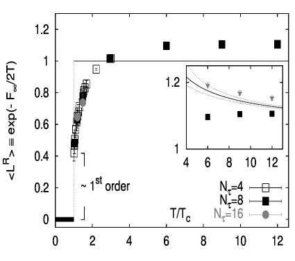
Figure 1: The renormalized Polyakov loop expectation value as defined in (5) calculated on lattices of size $32^{3}\times 4,8,16$. The matching to the zero temperature potential utilizes the standard Cornell form ($c=0$). The inserted figure shows a comparison of $\langle L^{R}\rangle$ for the case $c=0$ (squares) and $c=-T_{c}$ (triangles) at $T\raise 1.29167pt\hbox{$>$\kern-7.5pt\raise-4.73611pt\hbox{$\sim$}}6T_{c}$ to (continuum) 1-loop perturbation theory.

Lattice results[5] of the renormalized Polyakov loop are shown in Fig. 1. The renormalized Polyakov loop expectation value acts as an order parameter for the confinement-deconfinement phase transition and is well behaved in the continuum limit. At high temperatures, $\langle L^{R}\rangle$ approaches values larger than unity, which is supposed to be its high temperature limit. However, the renormalized Polyakov loop depends (multiplicatively) on the fixing of the zero-T potential. In order to demonstrate this dependence and to study contact with perturbation theory[8] we have inserted data with different fixing constants, $c=0$ and $c=-T_{c}$ (see inserted figure). Although the renormalization scheme depends on this fixing, the renormalized Polyakov loop expectation value approaches an ’universal’ value at large temperatures: Indeed, for different $c$ and $\tilde{c}$ it follows $\lim_{T\to\infty}\langle L^{R}_{(\tilde{c})}\rangle=\lim_{T\to\infty}\langle L^{R}_{(c)}\rangle$. Since a shift of the zero temperature potential corresponds to a non-perturbative contribution in the renormalized Polyakov loop $<L^{R}\rangle$ we expect the renormalized Polyakov loop to coincide with (continuum) perturbation theory at high temperatures where the shift does not influence the magnitude of $\langle L^{R}\rangle$. We therefore also expect that the renormalized Polyakov loop defined in our scheme approaches unity at infinite temperature.

$\beta\equiv 6/g^{2}$	4.100	4.127	4.154	4.179	4.200	4.229
$N_{\tau}=4$	1.367(2)	1.368(3)	1.367(3)	1.368(2)	1.368(2)	1.369(2)
$\beta\equiv 6/g^{2}$	4.321	4.343	4.365	4.400	4.600	4.839
$N_{\tau}=4$	1.367(2)	1.366(1)	1.365(1)	1.364(1)	1.349(1)	1.329(1)
$\beta\equiv 6/g^{2}$	4.5592	4.6605	4.8393	5.4261	6.0434	6.6450
$N_{\tau}=8$	1.355(1)	1.346(1)	1.330(1)	1.283(4)	1.242(2)	1.209(1)

Figure 2: The non-perturbatively determined renormalization constant defined through $Z_{(0)}^{R}=(\langle L^{R}_{(0)}/\langle L\rangle)^{1/N_{\tau}}$.

The renormalization constant for the Polyakov loop can be estimated in terms of $(\langle L^{R}\rangle/\langle L\rangle)^{1/N_{\tau}}$. We only note here, that the values of $Z^{R}$ (see Fig. 2) are independent of the lattice extent in time direction and compensate the divergence appearing in (2). For small couplings $g^{2}$, $\beta\equiv 6/g^{2}\in[4.8,6.6]$, the data for $Z^{R}$ can be well described with a function $f(g^{2})=\exp(Q_{2}(8/3)g^{2}+Q_{4}g^{4})$ with $Q_{2}=0.106$ and $Q_{4}=-0.065$. These values are of the same magnitude as they appear in lattice perturbation theory[2].

4 Conclusion

We have shown that the non-perturbative renormalization scheme applies to $n$-point Polyakov loop correlation functions once having fixed the renormalization constant for one of these correlation functions. This can, for instance, be done for the simplest Polyakov loop correlation function, the $2$-point function which describes the quark-anti-quark free energy. The renormalization of the free energies is equivalent to having fixed the corresponding partition function from which other physical quantities like the potential energy[7] can now be deduced.

References

- [1] L. G. McLerran and B. Svetitsky, Phys. Rev. D24 (1981) 450.
- [2] U. Heller and F. Karsch, Nucl. Phys. B251 (1985) 254.
- [3] For a recent discussion and further references see also: P. de Forcrand and L.v. Smekal, Phys. Rev. D66-011504 (2002), hep-lat/0107018.
- [4] A. Dumitru and R.D. Pisarski, Phys. Lett.B525 (2002) 95.
- [5] O. Kaczmarek et al., Phys. Lett. B543 (2002) 41.
- [6] S. Necco and R. Sommer, Nucl. Phys. B622 (2002) 328.
-
[7]
F. Zantow et al., hep-lat/0301015; contribution to
SEWM-2002
(this conference). - [8] E. Gava and R. Jengo, Phys. Lett. B105 (1981) 285.