The electrical conductivity and soft photon emissivity of the QCD plasma

Abstract

The electrical conductivity in the hot phase of the QCD plasma is extracted from a quenched lattice measurement of the Euclidean time vector correlator for $1.5\leq T/T_{c}\leq 3$. The spectral density in the vicinity of the origin is examined using a method specially adapted to this region, and a peak at small energies is seen. The continuum limit of the electrical conductivity, and the closely related soft photon emissivity of the QCD plasma, are then extracted from a fit to the Fourier transform of the temporal vector correlator.

The soft photon production rate from the plasma phase of hadronic matter is of importance to searches for the QCD phase transition wa98 . Consequently, there has been a long history of attempts at perturbative computations of this rate history . The first lattice prediction of dilepton (off-shell photon) rates was performed a while back dilepton . Recently the leading order computation of the photon production rate was completed amy . The Kubo formula relates the soft limit of this rate to the DC electrical conductivity of the QCD plasma, $\sigma$. To leading log accuracy in the gauge coupling, $g=\sqrt{4\pi\alpha_{\scriptscriptstyle S}}$, one has $\sigma\propto\alpha T/g^{4}\log g^{-1}$, where $\alpha$ is the fine structure constant. The proportionality constant has been computed recently in the leading-log approximation amy2 . Here we report the first computation of $\sigma$ and the soft photon emissivity from a quenched lattice computation in a region of temperature where $g$ is large and the weak-coupling approach fails amynote . Our methods can also be applied to other transport problems.

The photon emissivity at temperature $T$ is related to the imaginary part of the retarded photon propagator, i.e., the spectral density, $\rho_{\scriptscriptstyle EM}^{\mu\nu}$, for the electromagnetic current correlator, through the relation

$$\omega\frac{d\Omega}{d^{3}{\mathbf{p}}}=\frac{1}{8\pi^{3}}n_{\scriptscriptstyle B}(\omega,T){\rho_{\scriptscriptstyle EM}}_{\mu}^{\mu}(\omega,{\mathbf{p}},T).$$ (1)

In this work we shall take $\omega={\mathbf{p}}=0$, and hence obtain the soft photon production rate. Since the EM Ward identity gives $\rho^{00}(\omega,{\mathbf{0}},T)=0$, this soft limit is related to transport properties of the QCD plasma through the Kubo formula,

$$\sigma(T)=\frac{1}{6}\left.\frac{\partial}{\partial\omega}{\rho_{\scriptscriptstyle EM}}_{i}^{i}(\omega,{\mathbf{0}},T)\right|_{\omega=0},$$ (2)

where the sum is over spatial polarisations. A lattice determination of this rate proceeds from the spectral representation for Euclidean current correlators—

$$G_{\scriptscriptstyle EM}(t,{\mathbf{p}},T)=\int_{0}^{\infty}\frac{d\omega}{2\pi}K(\omega,t,T)\rho_{\scriptscriptstyle EM}(\omega,{\mathbf{p}},T),$$ (3)

where the integral kernel $K=\exp(\omega t)n_{\scriptscriptstyle B}(\omega,T)+\exp(-\omega t)[1+n_{\scriptscriptstyle B}(\omega,T)]$. $G_{\scriptscriptstyle EM}$ is the product of the vector correlator summed over all polarisations, $G_{\scriptscriptstyle V}$, and the EM vertex factor $C_{\scriptscriptstyle EM}=4\pi\alpha\sum_{f}e_{f}^{2}$, where $e_{f}$ is the charge of a quark of flavour $f$. On discretising the integral it becomes clear that the extraction of $\rho_{\scriptscriptstyle EM}$ from the lattice computation of $G_{\scriptscriptstyle EM}$ is akin to a linear least squares problem. The complication is that the (potentially infinite) number of parameters to be fitted exceeds the number of data points (which is half the number of lattice sites in the time direction, $N_{t}$). The solution is to constrain the function $\rho_{\scriptscriptstyle EM}$ through an informed guess baym , and use a Bayesian method to extract it nullsp . The Maximum Entropy Method (MEM) gubernatis ; asakawa along with a free-field theory model of the spectral function has been used in the past dilepton . The hard dilepton rate for $\omega/T\geq 4$ is fully under control, with lattice and perturbation theory in good agreement dilepton . For that reason we concentrate here on the electrical conductivity and the soft photon rate.

Correlators were investigated at $T=1.5T_{c}$, $2T_{c}$ and $3T_{c}$ in quenched QCD. The temperature range is realistic for heavy-ion collisions. However, $g>1$ in this entire range of temperature precise and is therefore ineffective in the separation of length scales upon which weak-coupling approaches depend. In order to make continuum extrapolations, the computations were performed on a sequence of lattice spacings, $a=1/8T$, $1/10T$, $1/12T$ and $1/14T$, (i.e., $N_{t}=8$, 10, 12 and 14). Quark mass effects were controlled by working with staggered quarks of masses $m/T_{c}=0.03$ and $0.1$. Details of the runs, statistics, and the generation of configurations for $N_{t}<14$ are described in gavai . For these lattice spacings the computations were performed on two different spatial volumes in order to control finite volume effects. For $N_{t}=14$ we have added runs on $14\times 30^{3}$ lattices for $T=1.5T_{c}$ and $2T_{c}$, and on $14\times 44^{3}$ lattices for $T=3T_{c}$, generating 50 configurations separated by 500 sweeps each. We have measured vector correlators with two degenerate flavours of quarks. It has been demonstrated recently that in this limit the charged and uncharged vector correlators are identical nf11 .

Small but statistically significant differences between the lattice results and ideal quark gas predictions for $G_{\scriptscriptstyle EM}$ are observed at all temperatures, lattice spacings, quark masses and volumes investigated. In any lattice computation, we expect the high frequency part of $\rho_{\scriptscriptstyle EM}$ to contain lattice artifacts. Moreover, physics at momenta of order $1/a$ is perturbative short and not of interest in the present context. We remove this physics by taking the difference between the Euclidean temporal propagators in QCD and an ideal quark gas (free field theory) on the same lattice—

$$\Delta G_{\scriptscriptstyle EM}(\omega)=G_{\scriptscriptstyle EM}^{\scriptscriptstyle QCD}(\omega)-G_{\scriptscriptstyle EM}^{ideal}(\omega),$$ (4)

A subtraction is needed to remove the $\omega^{2}$ divergent pieces from the dispersion relations hilg . Other benefits accruing from this are discussed later.

We have estimated the spectral density by two classes of methods. The first class of general techniques consist of discretising the integral in eq. (3) into $N_{\omega}$ energy bins and rewriting the equation in the form $G_{\scriptscriptstyle EM}=K\rho_{\scriptscriptstyle EM}$ where $K$ is now an $N_{t}\times N_{\omega}$ matrix, $G_{\scriptscriptstyle EM}$ the data vector of length $N_{t}$ and $\rho_{\scriptscriptstyle EM}$ represents a vector of length $N_{\omega}$ integ . For $N_{\omega}>N_{t}$ the solution is non-unique. Additional constraints, called priors, must then be imposed to determine them ill . The extraction of the spectral density is performed in the context of Bayesian parameter extraction. Given the data on $G$, the probability distribution function for $\rho$ can be written using Bayes’ formula

$$P(\rho|G)=P(G|\rho)P(\rho)/P(G),$$ (5)

where $P(A|B)$ denotes the conditional probability of $A$ given $B$. The probability distribution function $P(\rho)$ contains the prior information on $\rho$ that is needed for the analysis. Writing $P(\rho|G)=\exp[-F(\rho)]$, the maximum likelihood analysis of the probability reduces to the problem of minimizing $F$. Since $P(G)$ is independent of $\rho$, this problem can be formulated as a minimisation of the function

$$F(\rho)=(G-K\rho)^{T}\Sigma^{-1}(G-K\rho)+\beta U(\rho),$$ (6)

where the first term is the logarithm of $P(G|\rho)$ and $P(\rho)=\exp[-\beta U]$. The superscript $T$ denotes a transpose, $\Sigma$ is the covariance matrix of the data, and $\beta$ is a non-negative parameter whose choice is specified later.

The MEM technique consists of choosing some vector $\rho_{\scriptscriptstyle EM}^{0}$ and defining $U(\rho_{\scriptscriptstyle EM})=\sum_{i}\rho_{\scriptscriptstyle EM}^{i}[\log(\rho_{\scriptscriptstyle EM}^{i}/\rho_{\scriptscriptstyle EM}^{0\,i})-1]$, where the sum is over components of the vectors. In previous works the prior $\rho_{\scriptscriptstyle EM}^{0}$ has been chosen to be the vector spectral function in an ideal quark gas dilepton . Another whole class of techniques is obtained by choosing $U(\rho_{\scriptscriptstyle EM})=[{\cal L}(\rho_{\scriptscriptstyle EM}-\rho_{\scriptscriptstyle EM}^{0})]^{2}$ where ${\cal L}$ is a non-singular matrix. The choices ${\cal L}=1$, $D$ and $D^{2}$ (where $D$ is a discretisation of the derivative) have been suggested in the literature. ${\cal L}=1$ is the model that $\Delta\rho_{\scriptscriptstyle EM}\equiv\rho_{\scriptscriptstyle EM}-\rho_{\scriptscriptstyle EM}^{0}=0$ except as forced by the data, ${\cal L}=D$ makes the a priori choice that $\Delta\rho_{\scriptscriptstyle EM}$ is constant and ${\cal L}=D^{2}$ is the prior choice of smooth $\Delta\rho_{\scriptscriptstyle EM}$ honerkamp .

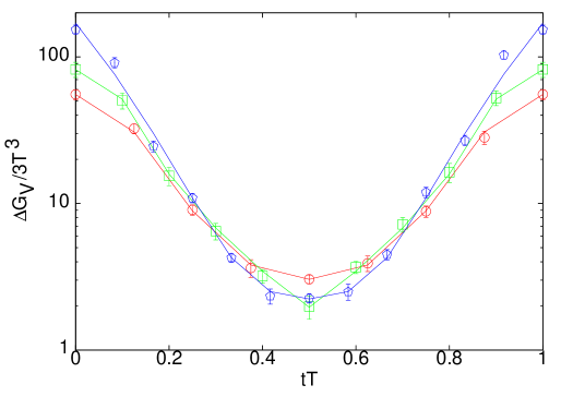
Figure 1: Bayesian fits to $\Delta G_{\scriptscriptstyle V}(t)$ at $T=2T_{c}$ for $m/T_{c}=0.03$ and $N_{t}=8$ (circles) 10 (squares) and 12 (pentagons). The fits were made with $N_{\omega}=16$ and $0\leq\omega\leq 4\pi T$, choosing ${\cal L}=1$. Changes in the fits due to variations in these algorithmic quantities are indistinguishable on the scale of this figure.

Such regulators have the added advantage that minimisation of the function $F$ in eq. (6) yields the linear problem—

$$\left[K^{T}\Sigma^{-1}K+\beta{\cal L}^{T}{\cal L}\right]\rho_{\scriptscriptstyle EM}=K^{T}\Sigma^{-1}G_{\scriptscriptstyle EM}+\beta{\cal L}^{T}{\cal L}\rho_{\scriptscriptstyle EM}^{0}.$$ (7)

Since ${\cal L}^{T}{\cal L}$ is positive definite, it is clear that the term in $\beta$ on the left hand side regulates the problem, by adding a term to $K^{T}\Sigma^{-1}K$ which makes the sum invertible. Since, for a well-determined parameter fitting problem, the value of $F$ is the $\chi^{2}$ value, we choose a value of $\beta$ at which $F=N_{t}$ at the minimum of $F(\beta)$, i.e., at the maximum a posteriori probability.

Considering the Bayesian problem as a field theory for the function $\rho_{\scriptscriptstyle EM}$, the method of maximising the a posteriori probability is equivalent to a semi-classical solution. The advantage of choosing a linear regulator is two fold. First, the search for the minimum is simply the solution of a system of linear equations; in non-linear minimisation it is no simple matter to correctly identify the global minimum press . Second, the linear problem is guaranteed to have a single minimum, whereas a general non-linear regulator may have multiple local minima, leading to complications analogous to the physics of phase transitions.

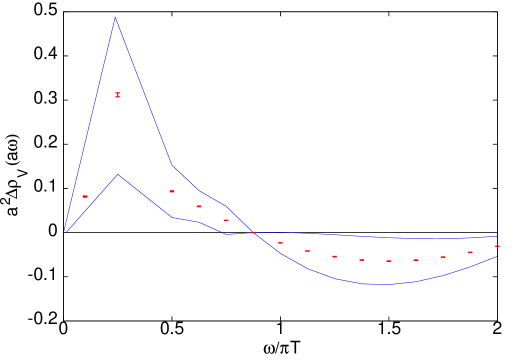
Figure 2: $\Delta\rho_{\scriptscriptstyle V}(\omega)$ obtained from fits to $\Delta G_{\scriptscriptstyle V}(t)$ at $T=2T_{c}$ determined on a $12\times 26^{2}\times 48$ lattice with $m/T_{c}=0.03$. Statistical errors obtained with $N_{\omega}=32$ are denoted by the bars, while the lines span thrice the range allowed by various systematic uncertainties as discussed in the text.

Since previous work has demonstrated that for $\omega\gg T$ lattice computations match perturbation theory dilepton , we focus our attention on the region $\omega\leq\pi T$. The linear relation between $G_{\scriptscriptstyle EM}$ and $\rho_{\scriptscriptstyle EM}$ means that we can assume $\rho_{\scriptscriptstyle EM}=\rho_{\scriptscriptstyle EM}^{0}+\Delta\rho_{\scriptscriptstyle EM}$, where $\rho_{\scriptscriptstyle EM}^{0}$ is the usual MEM prior in an ideal quark gas. At small $\omega$ this goes to zero faster than linearly in $\omega$ and hence does not contribute to $\sigma/T$ deltafoot . By choosing to work with $\Delta G_{\scriptscriptstyle EM}$, this $\rho_{\scriptscriptstyle EM}^{0}$ is removed from the problem, and we are freed to concentrate on the piece $\Delta\rho_{\scriptscriptstyle EM}$, which contains all the information needed to extract $\sigma$. Then in eq. (7) we use ${\cal L}=1$, replace $G_{\scriptscriptstyle EM}$ by $\Delta G_{\scriptscriptstyle EM}$ and $\rho_{\scriptscriptstyle EM}$ by $\Delta\rho_{\scriptscriptstyle EM}$, and remove the term in $\rho_{\scriptscriptstyle EM}^{0}$. The upper limit of the integral was truncated to $\omega=2n\pi T$ and the range divided into an uniform mesh of $N_{\omega}$ points. Varying $n$ and $N_{\omega}$ independently in the range $2\leq n\leq 4$ and $16\leq N_{\omega}\leq 64$ has no effect on the quality of the fit to the data (see Figure 1).

Statistical errors on $\Delta\rho_{\scriptscriptstyle EM}$ are assigned by a bootstrap over the measured values of $\Delta G_{\scriptscriptstyle EM}$. These are minor compared to uncertainties arising from algorithmic parameters. The latter are estimated by changing the integration method which is used to discretise eq. (3), the bin size in the integration, the integration limit, $N_{\omega}$, and the Bayesian prior specified by the matrix ${\cal L}$. Thrice the combined uncertainty due to these four factors is shown as the band in Figure 2 within which $\Delta\rho_{\scriptscriptstyle EM}$ lies. Even with this generous allowance for uncertainties there seems to be a peak in the spectral function at small $\omega$. For $\omega\geq\pi T$ the spectral function is roughly consistent with free field theory, but there is some evidence of a further peak at $\omega\approx 16\pi T$. The most important systematic uncertainty turns out to be related to control over the limit $a\to 0$. We found that the position of the peak and the slope at the origin change in going from $N_{t}=8$ to 14. This phenomenon has been noticed earlier in the context of MEM limit . A method which allows for better control of the continuum limit is required.

For this we utilize a second class of Bayesian methods, in which the prior is a model of the observed bump in the soft part of the spectrum. Since $\rho_{\scriptscriptstyle EM}$ is real and non-singular for real $\omega$, odd in $\omega$, and non-negative for $\omega>0$, one can choose to work with the most general form which gives rise to a non-vanishing electrical conductivity,

$$\frac{1}{T^{2}}\Delta\rho_{\scriptscriptstyle EM}(z)=\frac{z\sum_{n=0}^{N}\gamma_{n}z^{2n}}{1+\sum_{m=1}^{M}\delta_{m}z^{2m}},$$ (8)

where $z=\omega/T$ and with all $\gamma_{n}$ and $\delta_{m}$ real and non-negative aarts . The constraint that $\Delta\rho_{\scriptscriptstyle EM}\to 0$ at large $\omega$ is imposed by choosing $M>N$ param . We shall use the notation $(N,M)$ to denote a particular choice of $N$ and $M$. Bayesian techniques for parameter estimation then proceed by choosing a priori probability distributions for each parameter lepage .

The parameters in eq. (8) are most conveniently extracted by fitting to the Fourier transform of eq. (3) over the Euclidean time $t$ dolan

$${\cal G}_{\scriptscriptstyle EM}(\omega_{n},{\mathbf{p}},T)=\oint\frac{d\omega}{2i\pi}\frac{\rho_{\scriptscriptstyle EM}(\omega,{\mathbf{p}},T)}{\omega-\omega_{n}},$$ (9)

where the Euclidean frequencies are $\omega_{n}=2in\pi T$, ($1\leq n\leq N_{t}$ on a lattice) and the path of integration over complex $\omega$ runs over the real line and is closed in the upper half-plane. The form of $\rho_{\scriptscriptstyle EM}$ in eq. (8) can then be used to express the Fourier coefficients in terms of the parameters, which can be determined either through a least squares method if $1+N+M<N_{t}/2$, or a Bayesian method when there are more parameters than data.

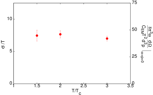
Figure 3: The electrical conductivity of the QCD plasma, $\sigma$, as a function of the temperature, $T$. The dimensionless quantity related to the soft photon emission rate shown on the right hand y-axis equals $6\sigma/T$ deltafoot . The bars denote statistical errors in the fit to the form in eq. (8) with $M=2$ and $N=1$.

A particular simplification occurs for $(0,M)$, since $\gamma_{0}$ is the only parameter that contributes for $\omega_{n}=0$. In all these cases $\sigma/T=C_{\scriptscriptstyle EM}(\chi_{\scriptscriptstyle V}-\chi_{\scriptscriptstyle V}^{0})/3T^{2}$, where $\chi_{\scriptscriptstyle V}={\cal G}_{\scriptscriptstyle V}(0,{\mathbf{0}},T)$ is the vector meson susceptibility gupta obtained in QCD and $\chi_{\scriptscriptstyle V}^{0}$ is the same quantity for an ideal quark gas on the same lattice arvind . Since the remaining parameters do not appear in this expression, their prior probabilities can be integrated out of the problem, without any assumptions about them. Such a marginalisation of the prior distribution is a general technique which has been demonstrated on other problems in the past for .

The extraction using $N=0$ must be insufficient for $T>10^{11}T_{c}$, since it does not reproduce the parametric dependence of $\sigma$ on $g$ in weak-coupling theory, which is expected to work at these temperatures. This can be improved by allowing for other values of $(N,M)$. We have investigated the stability of our results by going to $(1,2)$. Such a multiparameter fit moves the result up by 7%, which is within the statistical uncertainty. The electrical conductivity is thus reasonably stable, although it would be interesting in future to investigate its stability further, especially by using larger values of $N_{t}$.

In principle, such an extraction of parameters other than $\gamma_{0}$ in eq. (8), allows us to proceed beyond the $\omega=0$ limit of the dilepton rate. As more parameters are determined, the shape of the soft dilepton spectrum is also better constrained. An interesting open question is of the number of Fourier coefficients needed to fix the shape of the dilepton spectrum. This question is related to the stability of the transport coefficient, and we plan a study in the near future to address this question.

The estimates of $\sigma$ from the formula above are subject to lattice artifacts of order $a^{2}$ coming from ${\cal G}_{\scriptscriptstyle V}$. The continuum limit can then be obtained by an extrapolation in $1/N_{t}^{2}$. Finite volume effects turn out to be invisible within errors. Nor is there any visible quark mass dependence for small quark masses, since $m/T_{c}=0.03$ and $0.1$ give identical results within errors. We estimate $\sigma/T\approx 7C_{\scriptscriptstyle EM}$ in the continuum limit of the temperature range we studied. Finally, have used the estimate of $\sigma$ to predict the soft photon emissivity of the QCD plasma in equilibrium, as shown in Figure 3.

In summary, we adopted a sequence of Bayesian techniques for the inverse problem of extracting spectral densities, $\rho_{\scriptscriptstyle EM}$. In view of the results of dilepton we used the dispersion relations for Euclidean propagators after subtraction of the ideal gas values of the Euclidean temporal correlator, $\Delta G_{\scriptscriptstyle EM}$. We observed that in the QCD plasma, in the temperature range $1.5\leq T/T_{c}\leq 3$, the spectral density is peaked at small energies. This peak was next analyzed using a parametrised form of the Bayesian prior and the electrical conductivity of the plasma was extracted. This was then used to predict the soft photon emissivity of the QCD plasma.

Rough estimates of typical transport related time and length scales in the QCD plasma can be obtained by using the extracted value of the electrical conductivity in conjunction with the simple transport formula $\sigma=C_{EM}n_{q}\tau_{q}/m$ ($C_{EM}$ is nothing but the average charge square: $e^{2}$). If the number density of quarks, $n_{q}$, is substituted by the corresponding entropy density, and the screening mass used for $m$, then one finds the quark mean free time $\tau_{q}\approx 0.3$ fm. This is also the time scale for the persistence of charge, isospin, strangeness and baryon number fluctuations in the plasma amy2 . A possible experimental check could be to determine the mean free path of very soft off-shell photons ($\omega\ll 0.15(2\pi T)\approx 200$ MeV). These are only 20 times longer than $\tau_{q}$, i.e., about 6 fm. The fireball at RHIC may be marginally transparent to such photons, but at LHC the fireball size could be large enough to attenuate the intensity of very soft photons. Such an observation would constitute direct evidence for short mean free paths in the plasma.

Some estimates of other transport coefficients can be obtained if one assumes that the mean free time of gluons is $\tau_{q}/2$, since they should be related by colour factors. Then simple transport formulæ treated in the same approximation as before lead us to the estimate that the dimensionless ratio $\eta/S\approx 0.2$, where $S$ is the entropy density of the plasma and $\eta$ is the shear viscosity. This ratio is of the same order of magnitude as extracted from present heavy-ion data teany and obeys a bound conjectured in son . It would be useful to make a direct measurement of the shear viscosity on the lattice.

Many interesting lines of research are relegated to the future. The dilepton emissivity away from $\omega=0$ is a conceptually simple extension, but requires further numerical work, as explained before. Extending these measurements closer toward $T_{c}$ where correlation lengths grow larger saumen is of obvious importance, but outside the scope of this paper, as is the extension to dynamical QCD. The interesting question of the effectiveness of linear response theory, and hence of the Kubo formulae closer to $T_{c}$, can perhaps be probed using the non-linear susceptibilities defined in zakopane .

References

- (1) R. Albrecht et al. (CERN WA80), Phys. Rev. Lett., 76 (1996) 3506; G. Agakishiev et al., (CERN NA45/CERES) Phys. Lett., B 422 (1998) 405; M. M. Aggarwal et al. (CERN WA98), Phys. Rev. Lett., 85 (2000) 3595.
- (2) See F. Gelis, Nucl. Phys., A 715 (2003) 329, for a recent review of the subject.
- (3) F. Karsch et al., Phys. Lett., B 530 (2002) 147. Of course, in a lattice computation this is dressed by all possible gluon and sea quark insertions, the latter being absent in the quenched approximation.
- (4) P. Arnold et al., J. H. E. P., 0111 (2001) 057.
- (5) P. Arnold et al., J. H. E. P., 0011 (2000) 001.
- (6) The leading-log approximation gives a negative value of , since , indicating the failure of the approximation. Dropping the logarithm to “cure” this problem is unfeasible because the expansion is organised in powers of the logarithm.
- (7) R. V. Gavai and S. Gupta, Phys. Rev., D 67 (2003) 034501.
- (8) L. P. Kadanoff and G. Baym, Quantum Statistical Mechanics, W. A. Benjamin, New York (1962).
- (9) The integral on the right of eq. (3) could admit a non-trivial kernel, i.e., there could be a class of non-vanishing functions for which the integral vanishes. However they must necessarily change sign at least once, and we exclude them from the class of admissible spectral functions. In this restricted space, eq. (3) is invertible in the continuum limit. See also baym .
- (10) M. Jarrell and J. E. Gubernatis, Phys. Rep., 269 (1996) 133.
- (11) Y. Nakahara et al., Phys. Rev., D 60 (1999) 091503; M. Asakawa et al., Prog. Part. Nucl. Phys., 46 (2001) 459; I. Wetzorke et al., Nucl. Phys. Proc. Suppl., 106 (2002) 510.
- (12) S. Gupta, Phys. Rev., D 64 (2001) 034507.
- (13) R. V. Gavai and S. Gupta, Phys. Rev., D 66 (2002) 094510.
- (14) G. P. Lepage and P. B. McKenzie, Phys. Rev., D 48 (1993) 2250
- (15) J. Hilgevoord, Dispersion Relations and Causal Description, North-Holland, Amsterdam (1960).
- (16) The discretisation of the integral is made using Newton-Cotes formulæpress . The weights due to the conversion of the integral to the sum are included in the matrix .
- (17) W. H. Press et al., Numerical Recipes, Cambridge University Press, Cambridge, (1989).
- (18) A. N. Tikhonov and V. Y. Arsenin, Solutions of Ill-posed Problems, Wiley, New York (1977); M. M. Lavrent’ev et al.. Ill-posed Problems of Mathematical Physics and Analysis, Translations of Mathematical Monographs, Vol. 64, American Mathematical Society, Providence (1986).
- (19) For a comparison of the different methods, see, for example, J. Honerkamp, Statistical Physics, Springer, Berlin (2002).
- (20) The photon production rate in eq. (1) contains an extra term in which vanishes but can be shown formally to be of the form , where is the charge susceptibility measured in gavai . In the rest of this paper we treat this rate without this piece. It should be added in applications where it is needed.
- (21) M. Asakawa et al., Nucl. Phys., A 715 (2003) 863.
- (22) G. Aarts and J. M. M. Resco, J. H. E. P., 0204 (2002) 053, and hep-lat/0209033. is sufficient for positivity of ; reflection symmetry in the real and imaginary axes of the zero and pole sets is necessary and sufficient. For the conditions on the zero set are even weaker.
- (23) F. Karsch and H. W. Wyld, Phys. Rev., D 35 (1987) 2518 and S. Sakai et al., hep-lat/9810031, use a relaxation time approach which corresponds to taking and for .
- (24) G. P. Lepage et al., Nucl. Phys., B (Proc. Suppl.) 106 (2002) 12.
- (25) L. Dolan and R. Jackiw, Phys. Rev., D 9 (1974) 3320.
- (26) W. J. Fitzgerald and J. J. K. Ó Ruanaidh, Numerical Bayesian Methods Applied to Signal Processing, Springer, Heidelberg (1996).
- (27) S. Gupta Phys. Lett., B 288 (1992) 171.
- (28) Considering as a function of the poles of eq. (8) one proves that it is bounded as the poles go to zero or infinity in separate groups. The value of this function can then be obtained by induction. I would like to thank T. Ramadas and Arvind Nair for suggesting the method of proof.
- (29) D. Teaney, Phys. Rev., C 68 (2003) 034913.
- (30) P. Kovtun, D. T. Son and A. O. Starinets, J. H. E. P., 0310 (2003) 064.
- (31) O. Kaczmarek et al., Phys. Rev., D 62 (2000) 034021; S. Datta and S. Gupta, Phys. Rev., D 67 (2003) 054503.
- (32) S. Gupta, Acta Phys. Polon., B 33 (2002) 4259; R. V. Gavai and S. Gupta, Phys. Rev., D68 (2003) 034506 and hep-lat/0309014.