Interactions between Lattice Hadrons H. Rudolf FiebigPhysics Department, FIU, Miami, Florida 33199, USA Harald MarkumAtominstitut, Technische Universität Wien, A-1040 Vienna, Austria

1 Abstract

The effective residual interaction for a system of hadrons has a long tradition in theoretical physics. It has been mostly addressed in terms of boson exchange models. The aim of this review is to describe approaches based on lattice field theory and numerical simulation. At the present time this subject matter is in an exploratory stage. A large array of problems waits to be tackled, so that known features of hadron-hadron interactions will eventually be understood in a model-independent way. The lattice formulation, being capable of dealing with the nonperturbative regime, describes strong-interaction physics from first principles, i.e. quantum chromodynamics (QCD). Although the physics of hadron-hadron interactions may be intrinsically complicated, the methods used in lattice simulations are simple: For the most part they are based on standard mass calculations. This chapter addresses commonly used techniques, within $\mbox{QCD}_{3+1}$ and also simpler lattice models, describes important results, and also gives some insight into numerical methods for multi-quark systems.

2 Introductory Overview on Goals, Strategies, and Methods

2.1 Modeling Nuclear Forces

The theory of nuclear forces was pioneered by Yukawa [1] in 1935. A particle of intermediate mass, a meson, accounts for the interaction energy of the proton and neutron. In the framework of a quantum field theory the meson appears as the quantum of an effective field that describes the strong interaction [2]. The approximate range of the interaction

$$R=\frac{\hbar c}{mc^{2}}$$ (1)

is roughly consistent with $R\approx 2~{}{\rm fm}$, for a meson mass in the region of $m\approx 100~{}{\rm MeV}$. Those numbers are crude estimates based on the uncertainty relation (for energy and time) and the contemporary experimental evidence.

An effective neutron-proton interaction can be obtained from solutions of the Klein-Gordon equation for the meson field $\varphi$

$$(\Box+m^{2})\varphi(x)=g{\bar{\psi}(x)}\psi(x)\,,$$ (2)

with the pion-nucleon coupling $g$. In the static limit, where the product of nucleon fields $\bar{\psi}\psi$ is replaced with a generic point-like source,

$$(-\Delta+m^{2})\varphi(\vec{r}\,)=g\delta(\vec{r}\,)\,,$$ (3)

the solution, i.e. the static Green function,

$$\varphi(x)=\frac{g}{4\pi}\frac{e^{-mr}}{r}$$ (4)

is interpreted as a potential energy function, the ‘Coulomb potential’ of the meson theory. (Units are such that $\hbar=c=1$, conversion is $\hbar c=0.197~{}\mbox{GeV\,fm}$.) This line of thought is in close analogy to electrodynamics where the Coulomb potential emerges as the solution of a Poisson equation with a static point-like charge (source).

Since the early work, the meson theory of nuclear forces has received much attention and refinements. One of the more significant insights [3] has been that the range of the nucleon-nucleon force can be subdivided into three regions:

• The long-range region, inter-nucleon distances are above $r\approx 1.5~{}\mbox{fm}$. Here we have attraction. This is the region described by the Yukawa potential.

• Intermediate-range attraction, around $r\approx 1.0~{}\mbox{fm}$.

• Short-range repulsion, below $r\approx 0.5~{}\mbox{fm}$.

Other salient features are:

• A tensor force, important for the quadrupole moment of the deuteron.

• The presence of a spin-orbit force.

• Charge independence of the strong interaction.

In order to describe the short-distance region, scalar and vector mesons ($\eta,\rho,\omega,\ldots$) are needed in the boson-exchange model. Remarkably, a $\pi$–$\pi$ correlated state (known as the $\sigma$ meson) is relied upon to produce intermediate range attraction. The pseudoscalar meson ($\pi$), which also gives rise to the long-range (though finite) Yukawa potential, contributes significantly to the tensor force.

After approximately half a century the meson theory of nuclear forces is at a mature, sophisticated stage. Exhaustive review articles exist, for example Refs. [4, 5, 6, 7] may serve the interested reader. Boson-exchange models of this type presently constitute the state-of-the-art for effective theories of nuclear forces.

Typical for this class of models is an effective Lagrangian, say for the nucleon-nucleon interaction, such as

$${\cal L}_{\bar{\psi}\varphi\psi} = \sum_{\varphi}\left(\rule{0.0pt}{14.22636pt}-g_{\rm P}\overline{\psi}i\gamma_{5}\psi\varphi^{\rm P}+g_{\rm S}\overline{\psi}\psi\varphi^{\rm S}\right.$$ (5)

$$\left.-g_{\rm V}\overline{\psi}\gamma_{\mu}\psi\varphi^{\rm V}_{\mu}-\frac{f_{\rm V}}{2M}\overline{\psi}\sigma^{\mu\nu}\psi\partial_{\mu}\varphi^{\rm V}_{\nu}\right)\,,$$

with pseudoscalar $g_{\rm P}$, scalar $g_{\rm S}$, vector $g_{\rm V}$ and tensor $f_{\rm V}$ couplings for the various bosons $\varphi$, and $M$ is the nucleon mass [7]. Potentials are obtained from tree-level diagrams to the nucleon-nucleon propagator. Those are most naturally written in momentum space. The simplest contribution derived from (5) is

$$V(\vec{k})=-\frac{g_{\rm P}^{2}}{12M}\left[\vec{\sigma}_{1}\cdot\vec{\sigma}_{2}-\vec{\sigma}_{1}\cdot\vec{\sigma}_{2}\frac{m_{\rm P}^{2}}{\vec{k}^{2}+m_{\rm P}^{2}}+\frac{S_{12}(\vec{k})}{\vec{k}^{2}+m_{\rm P}^{2}}\right]\vec{\tau}_{1}\cdot\vec{\tau}_{2}\ldots\,,$$ (6)

where $m_{\rm P}$ is the pseudoscalar mass. This already is the non-relativistic reduction where the three terms correspond to a (coordinate-space) $\delta$-function, a Yukawa, and a tensor potential, the latter containing

$$S_{12}=3(\vec{\sigma}_{1}\cdot\vec{k})(\vec{\sigma}_{2}\cdot\vec{k})-\vec{\sigma}_{1}\cdot\vec{\sigma}_{2}\vec{k}^{2}\,.$$ (7)

The momentum transfer is $\vec{k}=\vec{q}\,^{\prime}-\vec{q}$ and $\vec{\sigma}_{1}$, $\vec{\sigma}_{2}$ are the nucleon spins. In addition, for each type of coupling momentum cutoff form factors are included with the coupling constants $g_{\rm P},g_{\rm S},g_{\rm V}$ and $f_{\rm V}$, for example

$$g_{\rm P}^{2}\rightarrow g_{\rm P}^{2}\ \left(\frac{\Lambda_{\rm P}^{2}-m_{\rm P}^{2}}{\Lambda_{\rm P}^{2}+\vec{k}^{2}}\right)^{n_{\rm P}}\,.$$ (8)

The inverse of a momentum cutoff parameter $\Lambda_{\rm P}$ is a length, and as such indicates the region of validity of the model. Values of $\approx 1~{}{\rm GeV}$, or equivalently $\approx 0.2~{}{\rm fm}$ are typical. Other refinements of the model include isobar ($\Delta$) degrees of freedom, and the extension to the strange hadron sector [8, 9]. Typical potentials are illustrated in Fig. 1.

Figure 1: Generic form of a central nucleon-nucleon potential according to boson exchange models and its contribution from various bosons. Schematic drawing after Ref. [7].

The philosophy of boson exchange models is to take the phenomenology of low-energy excitations of the hadronic vacuum as a starting point. The experimentally known spectrum of mesons and hadrons is used to reconstruct the forces between those particles. The result is an effective theory with adjustable parameters and predictive power in a reasonably well-defined realm of validity. An example is shown in Fig. 2. Naturally, the question of how hadronic interaction results from the underlying microscopic structure of hadrons and the, as we now know, complicated structure of the hadronic vacuum, is beyond the scope, and aim, of the model.

Figure 2: Nucleon-nucleon scattering phase shift for channels ${}^{1}S_{0}$ and ${}^{1}D_{2}$ compiled from Ref. [10]. In the ${}^{1}D_{2}$ channel the smooth curve is a ‘Bonn-potential’ result.

In the present context we wish to look at hadronic interactions from the perspective of lattice QCD. Since the physics of hadronic interactions is contained in the low-energy, non-perturbative, regime of QCD the lattice formulation is well suited for this task.

2.2 The Lattice QCD Perspective

From the lattice QCD point of view the three-fold subdivision of the inter-nucleon interaction region, see Fig. 1, appears in a new light:

• The long-range region is expected to be dominated by excitations of the QCD vacuum that are recovered only in the chiral limit of the lattice simulation. If Wilson fermions are used this region can be monitored by extrapolating to the zero-mass limit of the pseudoscalar meson, which is the Goldstone boson of QCD. The mechanism for pion exchange is available on the lattice because correlated quark-antiquark pairs are dynamically provided by the lattice action. This is true even if the simulation is limited to the quenched approximation.

• In the intermediate-distance region various excitations of the QCD vacuum of somewhat higher mass will take over. Those may be pure hadronic states, gluonic excitations, or combinations of such. In contrast to boson exchange models the precise nature of those need not be known as input. Again those would be accounted for by the lattice action. At $r\approx 1.0~{}\mbox{fm}$ this is really a transition region between an appropriate description in terms of effective hadronic fields and the asymptotically free regime of the interior quark-gluon cores of the hadrons. The validity of traditional boson exchange models seems somewhat stretched here. With the currently available lattice constants ($\approx 0.1$ – $0.4~{}\mbox{fm}$) the intermediate-distance region appears appropriate for lattice QCD.

• For small distances the compositeness of the hadrons, as finite-size quark-gluon systems, will play the dominant role. Not surprisingly, quark models have been used to study the nucleon-nucleon interaction. The energies involved are naturally larger, for example $\approx 2~{}{\rm GeV}$, and thus point to lattice constants of about $\approx 0.1~{}{\rm fm}$, being not out of reach of contemporary lattice simulations. Lattice QCD provides dynamically for the compositeness of the hadrons. Internal hadronic structure is, in turn, crucial for the features of the residual interaction.

Thus lattice QCD is in a position to combine the classic nucleon-nucleon interaction regions in a single unified approach. Moreover, the strange hadron sector, or effects of strangeness in the light-quark sector are straightforwardly incorporated.

2.3 Short and Long Term Goals for Lattice QCD

While boson exchange models have a long tradition, attempts to study residual interactions between systems of hadrons within lattice QCD are only in an experimental stage. The physics of hadronic interactions in terms of first principles is rather involved, see Fig. 3. Conceptual, technical, and computational questions are very much in the foreground at this time. The tentative nature of this situation will be apparent throughout this chapter.

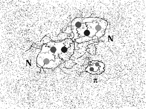
Figure 3: Cartoon of a strongly interacting hadron-hadron system from the QCD perspective.

Nevertheless, there is potential for new physics, or at least for understanding known phenomena in a new light. In particular, probing hadronic matter at somewhat higher energies, say in the 4 – 8 GeV region with electron beams, has become a new focus in experimental nuclear physics. The interest here lies in the boundary between particle (high energy) and nuclear (low energy) physics which we will refer to as hadronic physics. Our short-term working list is as follows:

• Discuss various basic concepts and numerical methods using simple lattice models.

• Study simple systems, mostly meson-meson, and extract non-relativistic potentials.

• Explore alternative approaches to the problem, like momentum space and coordinate space formulations.

As a long-term perspective we have in mind:

• Study realistic meson-meson, meson-baryon, and baryon-baryon systems. For example, the pion-nucleon system features the prominent delta resonance, a hallmark of strong-interaction physics.

• Residual interactions in the strange-hadron sector.

• Develop advanced methods, possibly the direct extraction of scattering amplitudes from the lattice.

2.4 Probing the Lattice

A hadron-hadron force may be viewed as a hyperfine interaction in the hadron-hadron system. In one way or another, we must therefore compare the mass spectrum of the interacting hadron-hadron system to the spectrum of the non-interacting hadron-hadron system.

About two decades ago it was realized that finite volume effects may in principle be exploited to achieve this end [11]. The energy levels of a two-hadron system, say two mesons with mass $m$ each, are subject to finite-size corrections. Those decrease with powers of $1/L$ as the lattice size $L$ increases. The formal study of finite-size effects in this context is due to Lüscher [12, 13]. In Ref. [13] the following equation for the ground-state two-body energy shift

$$W_{0}-2m=-\frac{4\pi a_{0}}{mL^{3}}\left\{1+c_{1}\frac{a_{0}}{L}+c_{2}\frac{a_{0}^{2}}{L^{2}}\right\}+o(L^{-6})$$ (9)

is derived. It is valid for s-wave elastic scattering, below the particle production threshold. Above $c_{1}=-2.837297$, $c_{2}=6.375183$, and $a_{0}$ is the s-wave scattering length. This result has been the basis for a number of studies [14, 15, 16, 17, 18, 19, 20, 21, 22, 23, 24, 25, 26]. The extraction of scattering information beyond the static limit, like phase shifts at nonzero relative energy, is formally more involved [27, 28].

In general it will be necessary to probe the lattice (vacuum) with one- and two-hadron operators. Let $\phi_{\vec{p}}(t)$ be a composite field, say, constructed from quark–antiquark (meson) or from three–quark (baryon) fields. Let $\vec{p}$ be the hadron momentum, for simplicity we disregard additional quantum numbers. The time correlation matrix built from one-hadron operators

$$C^{(2)}_{\vec{p}\,\vec{q}}(t,t_{0})=\langle\phi^{\dagger}_{\vec{p}}(t)\,\phi_{\vec{q}}(t_{0})\rangle-\langle\phi^{\dagger}_{\vec{p}}(t)\rangle\langle\phi^{\phantom{\dagger}}_{\vec{q}}(t_{0})\rangle$$ (10)

possesses eigenvalues $\lambda^{(2)}_{m_{1}}(t,t_{0})$ which behave exponentially,

$$\lambda^{(2)}_{m_{1}}(t,t_{0})\propto e^{-w_{m_{1}}(t-t_{0})}\,.$$ (11)

The time correlation matrix is just the euclidean version of a propagator, in our example a 2-point function $C^{(2)}$ on the hadronic level (a 4- or 6-point function on the quark level). Thus from (11) the energies $w_{m_{1}}$ of the one-meson system can be extracted. Typically, this is done numerically. A practical example is shown in Fig. 4. The interpretation of the $w_{m_{1}}$ is that those are energies of the hadron moving through the lattice. In principle, the hadron could be in an internally excited state.

Figure 4: Typical time correlation functions (eigenvalues) extracted from a lattice simulation. The examples are for a pseudoscalar meson (PSM) and a vector meson (VEC) using $\mbox{QCD}_{3+1}$ and Wilson fermions.

The fields $\Phi_{\vec{p}}(t)=\phi_{-\vec{p}}(t)\,\phi_{+\vec{p}}(t)$ can be used for probing two-hadron states. These are operators with total momentum $\vec{P}=0$. Note that $\vec{p}$ in this example means the relative momentum of the two-hadron system. We construct a 4-point correlation matrix

$$C^{(4)}_{\vec{p}\,\vec{q}}(t,t_{0})=\langle\Phi^{\dagger}_{\vec{p}}(t)\,\Phi_{\vec{q}}(t_{0})\rangle-\langle\Phi^{\dagger}_{\vec{p}}(t)\rangle\langle\Phi^{\phantom{\dagger}}_{\vec{q}}(t_{0})\rangle\,,$$ (12)

and, correspondingly, the eigenvalues

$$\lambda^{(4)}_{n}(t,t_{0})\propto e^{-W_{n}(t-t_{0})}$$ (13)

yield the energy levels $W_{n}$ of the two-hadron system. Most importantly, these levels somehow contain the desired residual interaction.

A sensible definition of the latter, of course, also involves the eigenvectors of $C^{(2)}$ and $C^{(4)}$, however, comparison of the level schemes

$$\{\overline{W}_{m=(m_{1},m_{2})}\stackrel{{\scriptstyle\rm def}}{{=}}w_{m_{1}}+w_{m_{2}}\}\quad\mbox{to}\quad\{W_{n}\}$$ (14)

already gives important insight into the nature of the hadron-hadron force.

Probing the lattice with momentum-type operators is only one of several alternatives. The use of coordinate space operators is another popular choice [29, 30, 31, 32, 33, 34, 35].

2.5 Finite-size Methods

The spectrum $\{W_{n}\}$ of the interacting two-body system may be utilized in a variety of ways. Lüscher has shown how to extract scattering phase shifts directly from the spectrum [28]. The idea is to match the poles of (interacting) Green functions that live on the finite-sized periodic lattice to the poles of (free) Green functions in infinite volume. Since the lattice Green functions comprise the interaction, comparison in the asymptotic (free) region yields the phase shifts. Using methods similar to the ‘Jost’ formalism of scattering theory [36] an equation of the following form

$$\det\left[e^{2i\delta}-(M+i)^{-1}(M-i)\right]=0$$ (15)

is derived. Here $M=M(q^{2})$ is an analytically constructed energy-dependent matrix ($W^{2}=m^{2}+q^{2}$). It reflects features of the ‘natural’ (free) spectrum of the periodic lattice. The other matrix $e^{2i\delta}$ in (15) contains a set of scattering phase shifts $\delta_{\ell}(q^{2})$. The lattice simulation gives a discrete spectrum $\{W_{n}\}$. A certain energy $W_{n}$, for a fixed $n$, is then used to calculate $M(q_{n}^{2})$ and (15) is solved for the corresponding $\delta_{\ell}(q_{n}^{2})$. This yields a set of phase shifts, as many as the size of $M$, at each energy $W_{n}$. The physical $\delta_{\ell}(q_{n}^{2})$, at a discrete $q_{n}^{2}$, is contained in this set.

A simple illustration of the idea behind this formalism [27] is the following: Consider a solution $\psi(x)$ of a Schrödinger equation in the noninteracting case with a phase $kL=2\pi\,n$. It satisfies $\psi(x)=\psi(x\!+\!L)$, see Fig. 5(a). If the interaction is turned on, say an attractive potential with range $|x|\leq 0.2L$, the periodic boundary condition would be violated, see Fig. 5(b), unless compensated for by a simultaneous change in the kinematical phase $kL$. In other words, the change in $kL$ necessary to restore the original periodic boundary conditions, see Fig. 5(c), is a measure for the phase shift.

Figure 5: Generic solutions $\psi(x)$ of a Schrödinger equation: (a) no interaction, (b) an attractive potential around $x\approx 0$, and (c) with decreased wave number $k$ to restore the original phase conditions.

The kinematical phase $kL$ is changed by varying $k$ or $L$. Varying $L$ is reminiscent of a finite-size effect, see (9). Finding the change in $k$ at fixed $L$ is equivalent to finding all (discrete) two-body levels $\{W_{n}\}$ for the interacting case. This method, which already appears in Ref. [13], has been used by Lüscher and Wolff [27] to obtain scattering phase shifts in an O(3) nonlinear sigma model on a 1+1 dimensional lattice.

2.6 Residual Interaction

Scattering phase shifts are very close to observable quantities (cross sections). This is an appealing feature of Lüscher’s method, as the above procedure came to be known. On the other hand an effective residual interaction between hadrons is more in line with the historic development and has a heuristic value which should not be underestimated. We will therefore place considerable emphasis on this aspect. In this approach the information contained in the 2- and 4-point correlation matrices, see (10) and (12), will be utilized in a different way.

In principle an effective residual interaction is subject to definition. Towards this end we will first split a free, or non-interacting, part off the 4-point correlation matrix (12)

$$C^{(4)}(t,t_{0})=\overline{C}(t,t_{0})+C_{I}(t,t_{0})\,,$$ (16)

where $\overline{C}$ is built from 2-point correlators $C^{(2)}$ and describes two non-interacting hadrons on the lattice. This can be accomplished by means of diagrammatic considerations. In terms of (16) we then define an effective residual interaction as

$$H_{I}=-\frac{\partial}{\partial t}\ln\left(\overline{C}^{\,-1/2}C_{I}\,\overline{C}^{\,-1/2}\right)\,.$$ (17)

In principle the interaction Hamiltonian (potential) is non-local. Our focus is to compute $H_{I}$ from a lattice simulation and eventually calculate the corresponding phase shifts.

The above method relies on lattice sizes large enough to accommodate two hadrons. Assuming a manageable lattice $L^{3}\times T$ with, say, $L=10$ and physical extent of about $4.0$ fm this translates into a lattice constant of $a=0.4$ fm. As experience with hadron spectroscopy has shown the standard Wilson plaquette action [37] requires $a\approx 0.1-0.2$ fm in order to work reasonably close to the continuum limit. This does not sound very encouraging for putting multi-hadron systems on the lattice.

2.7 Use of Improved Actions

Fortunately, considerable progress in recent years has provided us with so-called ‘improved’ lattice actions [38]. Here, in the simplest form, one supplements the Wilson action, built from elementary $1\times 1$ plaquettes (pl), with larger $1\times 2$ rectangles (rt)

$$S_{G}[U]=\beta\left(\rule{0.0pt}{9.0pt}S_{pl}[U]+c_{rt}S_{rt}[U]\right)\,.$$ (18)

The Wilson part of the action (pl) approaches the classical (tree-level) limit like $o(a^{4})$ as $a\rightarrow 0$. If $c_{rt}=-1/20$ the (rt) term in (18) improves this behavior to order $o(a^{5})$. We refer to such an action as $o(a)$ tree-level improved. Better yet, one can also account for a large part of the quantum fluctuations of the gluon field through renormalizing the link variables $U_{\mu}(x)$. Of course, this would destroy the tree-level cancellations between the (pl) and (rt) terms in (18). Within mean-field theory it can be ‘repaired’ by changing the factor $c_{rt}$ to

$$c_{rt}=-\frac{1}{20u^{2}}\,,$$ (19)

where $u$, known as the tadpole factor, is the fourth root of the average (4-link) plaquette

$$u=\langle\frac{1}{3}\mbox{Re}\,\mbox{Tr}\,U_{pl}\rangle^{1/4}\,.$$ (20)

The tadpole factor can easily be computed self-consistently within a running lattice simulation. There are also radiative corrections which can be incorporated into the lattice action to some extent [39, 40, 41].

The benefit of improvement is that the physical continuum limit, $a\rightarrow 0$, is approached ‘faster’ compared to the Wilson action. The ‘same physics’ is described with improved actions at larger lattice constants $a$. For example, a Wilson action at $a\approx 0.1$ fm may give a similar mass spectrum as an improved action at $a\approx 0.3$ fm. For our present purpose of putting two hadrons on the lattice, this means that, stretching things a bit and choosing $a\approx 0.4$ fm, we would only need an $L^{3}\times T$ lattice with about $L=10$ for a lattice of 4.0 fm across. This should give us a first window on two-hadron systems on the lattice.

Improved actions have been a big innovation for lattice field theory [42]. There are versions of improved actions including fermions [43], and work pushing the improvement to higher order, for example $o(a^{2})$ improved actions [44, 45, 46]. – In Appendix 8 we have collected some topics that are relevant to this chapter. – Strong-interaction physics, in particular the boundary between particle and nuclear physics, is now open to studies within quantum chromodynamics.

3 A Simple U(1) Lattice Model in 2+1 Dimensions

In order to discuss some practical work we look at a simple but non-trivial model. We consider U(1) gauge theory on an $L^{d}\times T$ lattice, in $d+1$ dimensions, with $d=2$. The intent is to study the interaction between two mesons living in a plane. For the sake of simplicity we work with the (unimproved) Wilson action and use staggered fermions.

3.1 Lattice Action

For a U(1) gauge group the link variables are

$$U_{\mu}(x)=e^{i\Theta_{\mu}(x)}\in\mbox{U(1)}\,,$$ (21)

with $\mu=1\ldots d+1$, $x=(\vec{x},t)$, and $\Theta_{\mu}(x)\in[-\pi,\pi)$. The plaquette (pl) variables are

$$U_{pl}(\mu,\nu;x) = U_{\mu}(x)U_{\nu}(x+\hat{\mu})U^{\dagger}_{\mu}(x+\hat{\nu})U^{\dagger}_{\nu}(x)$$ (22)

$$= \exp\left(\rule{0.0pt}{9.0pt}i\Theta_{pl}(\mu,\nu;x)\right)\,,$$

where

$$\Theta_{pl}(\mu,\nu;x)=\Theta_{\mu}(x)+\Theta_{\nu}(x+\hat{\mu})-\Theta_{\mu}(x+\hat{\nu})-\Theta_{\nu}(x)$$ (23)

is the oriented plaquette angle. We write $\hat{\mu}$ for a vector of length $a$ in direction $\mu$. The (compact form of the) Wilson gauge field action is

$$S_{G}=\beta\sum_{x}\sum_{\mu<\nu}\mbox{Re}\left(\rule{0.0pt}{9.0pt}1-U_{pl}(\mu,\nu;x)\right)=\beta\sum_{x}\sum_{\mu<\nu}\left(\rule{0.0pt}{9.0pt}1-\cos\Theta_{pl}(\mu,\nu;x)\right)\,.$$ (24)

For simplicity, fermions are treated in the staggered, or Kogut-Susskind, scheme where Dirac indices have been ‘spin-diagonalized’ away [47, 48, 49]. Thus we work with one-component Grassmann fields $\chi_{f}(x)$ defined on the lattice sites $x=(\vec{x},t)$, with (external) flavor index $f=u,d,s$. There is just one color index, $C=1$, which we omit. The fermionic action can be written as

$$S_{F}=\sum_{x,y}\sum_{f}\bar{\chi}_{f}(x)\>G^{-1}(x,y)[U]\,\chi_{f}(y)\,,$$ (25)

with the flavor-independent fermion matrix

$$G^{-1}(x,y)=\frac{1}{2}\sum_{\mu}\eta_{\mu}(x)\left[U_{\mu}(x)\delta_{x+\hat{\mu},y}-U^{\dagger}_{\mu}(y)\delta_{x,y+\hat{\mu}}\right]+m_{F}\,\delta_{x,y}\,,$$ (26)

including a mass term. Here $\eta_{\mu}(x)=(-1)^{x_{1}+\ldots x_{\mu-1}},\mu=2\ldots d+1,\eta_{1}(x)=1$ is the staggered phase.

This lattice field model is confining in finite volume [50], and exhibits chiral symmetry breaking [51] and monopole condensation [52], for appropriately chosen inverse gauge coupling $\beta$. Its basis is the euclidean generating functional integral

$$Z[\bar{J},J]=\int[dU][d\chi][d\bar{\chi}]e^{-S_{G}[U]-S_{F}[U,\chi,\bar{\chi}]+\bar{J}\chi+\bar{\chi}J}\,,$$ (27)

with the fermionic sources $\bar{J}\chi=\sum_{x}\bar{J}(x)\chi(x)$ and $\bar{\chi}J=\sum_{x}\bar{\chi}(x)J(x)$. We will use gauge configurations in the quenched approximation.

3.2 Meson Fields

The simplest hadrons we can work with are pseudoscalar mesons. In the staggered scheme suitable one-meson operators are

$$\phi_{\vec{p}}(t)=L^{-2}\sum_{\vec{x}}\,e^{i\vec{p}\cdot\vec{x}}\bar{\chi}_{d}(\vec{x},t)\,\chi_{u}(\vec{x},t)\,.$$ (28)

The $\vec{x}$ sum extends over the spatial sites of the lattice. The fixed flavor assignment $u$,$d$ leading to a $\pi^{+}$ will simplify computations. For $d=2$, a planar lattice, the momentum parameters are

$$\vec{p}=\frac{2\pi}{L}(k_{1},k_{2})\,,\quad\mbox{where}\quad k_{1,2}=-(\frac{L}{2}-1)\ldots\frac{L}{2}\,,\quad\mbox{even $L$}\,,$$ (29)

if $L$ is odd we have $k_{i}=-(L-1)/2\ldots(L-1)/2$. The operators (28) probe the lattice (vacuum) for composite meson states with momentum $\vec{p}$. Products of those operators probe for multi-meson excitations. For example

$$\Phi_{\vec{p}}(t)=\phi_{-\vec{p}}(t)\,\phi_{+\vec{p}}(t)$$ (30)

describes two-meson fields with total momentum $\vec{P}=0$ and relative momentum $\vec{p}$. The reduced mass is $m/2$.

3.3 Correlation Matrices

The time-correlation matrix for the one-meson system is

$$C^{(2)}_{\vec{p}\,\vec{q}}(t,t_{0})=\langle\phi^{\dagger}_{\vec{p}}(t)\,\phi_{\vec{q}}(t_{0})\rangle-\langle\phi^{\dagger}_{\vec{p}}(t)\rangle\langle\phi^{\phantom{\dagger}}_{\vec{q}}(t_{0})\rangle\,.$$ (31)

It can be worked out with Wick’s theorem in terms of contractions between the Grassmann fields. In our simple example we use, see Appendix 7,

$$\ldots\stackrel{{\scriptstyle n}}{{\chi}}_{f}(x)\stackrel{{\scriptstyle n}}{{\bar{\chi}}}_{f^{\prime}}(x^{\prime})\ldots = \ldots\delta_{ff^{\prime}}{G}(x,x^{\prime})\ldots$$ (32)

$$\ldots\stackrel{{\scriptstyle n}}{{\bar{\chi}}}_{f}(x)\stackrel{{\scriptstyle n}}{{\chi}}_{f^{\prime}}(x^{\prime})\ldots = \ldots\delta_{ff^{\prime}}{G}^{\ast}(x,x^{\prime})\ldots\,,$$ (33)

where ${n}$ indicates the partners of the contraction, and $G$ is the inverse fermion matrix, cf. (26). This may be used to work out the correlation matrices. For example, consider

$$\langle\phi^{\dagger}_{\vec{p}}(t)\,\phi_{\vec{q}}(t_{0})\rangle=L^{-4}\sum_{\vec{x}}\sum_{\vec{y}}\,e^{-i\vec{p}\cdot\vec{x}}e^{i\vec{q}\cdot\vec{y}}\langle\bar{\chi}_{u}(\vec{x},t)\chi_{d}(\vec{x},t)\,\bar{\chi}_{d}(\vec{y},t_{0})\chi_{u}(\vec{y},t_{0})\rangle\,.$$ (34)

Because of the flavor assignment in (28) the separable term in (31) is zero, and there is only one group of contractions in the first term

$$C^{(2)}\sim\;\;\,\stackrel{{\scriptstyle 2}}{{\bar{\chi}}}_{u}\,\stackrel{{\scriptstyle 1}}{{\chi}}_{d}\,\stackrel{{\scriptstyle 1}}{{\bar{\chi}}}_{d}\,\stackrel{{\scriptstyle 2}}{{\chi}}_{u}\,,$$ (35)

with

$$\ldots\stackrel{{\scriptstyle 1}}{{\chi}}_{d}(\vec{x},t)\stackrel{{\scriptstyle 1}}{{\bar{\chi}}}_{d}(\vec{y},t_{0})\ldots = \ldots G(\vec{x}t,\vec{y}t_{0})\ldots$$ (36)

$$\ldots\stackrel{{\scriptstyle 2}}{{\bar{\chi}}}_{u}(\vec{x},t)\stackrel{{\scriptstyle 2}}{{\chi}}_{u}(\vec{y},t_{0})\ldots = \ldots G^{\ast}(\vec{x}t,\vec{y}t_{0})\ldots\,.$$ (37)

Thus we obtain

$$C^{(2)}_{\vec{p}\,\vec{q}}(t,t_{0})=L^{-4}\sum_{\vec{x}}\sum_{\vec{y}}e^{-i\vec{p}\cdot\vec{x}+i\vec{q}\cdot\vec{y}}\langle|G(\vec{x}t,\vec{y}t_{0})|^{2}\rangle\,.$$ (38)

Assuming translational invariance

$$\langle|G(\vec{x},t;\vec{y},t_{0})|^{2}\rangle=\langle|G(\vec{x}+\vec{a},t;\vec{y}+\vec{a},t_{0})|^{2}\rangle$$ (39)

renders the 2-point correlator diagonal

$$C^{(2)}_{\vec{p}\,\vec{q}}(t,t_{0})=\delta_{\vec{p}\,\vec{q}}\;L^{-2}\sum_{\vec{x}}e^{-i\vec{p}\cdot\vec{x}}\langle|G(\vec{x}t,\vec{x}_{0}t_{0})|^{2}\rangle\,\,e^{i\vec{p}\cdot\vec{x}_{0}}\,.$$ (40)

The point $\vec{x}_{0}$ is arbitrary, $C^{(2)}$ is independent of $\vec{x}_{0}$, and the phase factor is irrelevant.

The 4-point correlator describes the propagation of two interacting mesons on the lattice

$$C^{(4)}_{\vec{p}\,\vec{q}}(t,t_{0})=\langle\Phi^{\dagger}_{\vec{p}}(t)\,\Phi_{\vec{q}}(t_{0})\rangle-\langle\Phi^{\dagger}_{\vec{p}}(t)\rangle\langle\Phi^{\phantom{\dagger}}_{\vec{q}}(t_{0})\rangle\,.$$ (41)

Here $\vec{p}$ and $\vec{q}$ are the relative momenta in the meson-meson system. In terms of the fermion propagator this correlator reads

$$C^{(4)}_{\vec{p}\,\vec{q}}(t,t_{0}) =L^{-8}\>\sum_{\vec{x}_{1}}\>\sum_{\vec{x}_{2}}\>\sum_{\vec{y}_{1}}\>\sum_{\vec{y}_{2}}\>{\rm e}^{i\vec{p}\cdot(\vec{x}_{2}-\vec{x}_{1})+i\vec{q}\cdot(\vec{y}_{2}-\vec{y}_{1})}$$

$$\mbox{}\left\langle\left(\>G^{\ast}(\vec{x}_{2}t,\vec{y}_{2}t_{0})\quad G(\vec{x}_{2}t,\vec{y}_{2}t_{0})\quad G^{\ast}(\vec{x}_{1}t,\vec{y}_{1}t_{0})\quad G(\vec{x}_{1}t,\vec{y}_{1}t_{0})\right.\right.$$

$$\mbox{}+G^{\ast}(\vec{x}_{1}t,\vec{y}_{2}t_{0})\quad G(\vec{x}_{1}t,\vec{y}_{2}t_{0})\quad G^{\ast}(\vec{x}_{2}t,\vec{y}_{1}t_{0})\quad G(\vec{x}_{2}t,\vec{y}_{1}t_{0})$$

$$\mbox{}-G^{\ast}(\vec{x}_{2}t,\vec{y}_{1}t_{0})\quad G(\vec{x}_{2}t,\vec{y}_{2}t_{0})\quad G^{\ast}(\vec{x}_{1}t,\vec{y}_{2}t_{0})\quad G(\vec{x}_{1}t,\vec{y}_{1}t_{0})$$

$$\mbox{}-\left.\left.G(\vec{x}_{2}t,\vec{y}_{1}t_{0})\quad G^{\ast}(\vec{x}_{2}t,\vec{y}_{2}t_{0})\quad G(\vec{x}_{1}t,\vec{y}_{2}t_{0})\quad G^{\ast}(\vec{x}_{1}t,\vec{y}_{1}t_{0})\right)\right\rangle\,.$$

For an SU(N) gauge group, $G\rightarrow G_{CC^{\prime}}$, there would be sums over four sets of color indices corresponding to the $\vec{x}_{1},\vec{x}_{2},\vec{y}_{1},\vec{y}_{2}$ assignment in (3.3). A diagrammatic classification of the various terms which contribute to $C^{(4)}$ proves useful. Such a classification arises naturally from working out the contractions between the quark fields in (41) and (31). Let us write

$$C^{(4)} = C^{(4A)}+C^{(4B)}-C^{(4C)}-C^{(4D)}$$ (43)

$$= \mbox{ \begin{picture}(18.0,17.0)\put(2.0,-6.0){\line(0,1){15.0}} \put(4.0,-6.0){\line(0,1){15.0}} \put(11.0,-6.0){\line(0,1){15.0}} \put(13.0,-6.0){\line(0,1){15.0}} \put(2.0,-6.0){\line(1,0){2.0}} \put(2.0,9.0){\line(1,0){2.0}} \put(11.0,-6.0){\line(1,0){2.0}} \put(11.0,9.0){\line(1,0){2.0}} \end{picture} }+\mbox{ \begin{picture}(18.0,17.0)\put(2.0,-6.0){\line(3,5){9.0}} \put(4.0,-6.0){\line(3,5){9.0}} \put(11.0,-6.0){\line(-3,5){9.0}} \put(13.0,-6.0){\line(-3,5){9.0}} \put(2.0,-6.0){\line(1,0){2.0}} \put(2.0,9.0){\line(1,0){2.0}} \put(11.0,-6.0){\line(1,0){2.0}} \put(11.0,9.0){\line(1,0){2.0}} \end{picture} }-\mbox{ \begin{picture}(18.0,17.0)\put(2.0,-6.0){\line(0,1){15.0}} \put(3.0,-6.0){\line(3,5){9.0}} \put(12.0,-6.0){\line(-3,5){9.0}} \put(13.0,-6.0){\line(0,1){15.0}} \put(2.0,4.0){\vector(0,1){0.0}} \put(2.0,-6.0){\line(1,0){1.0}} \put(2.0,9.0){\line(1,0){1.0}} \put(12.0,-6.0){\line(1,0){1.0}} \put(12.0,9.0){\line(1,0){1.0}} \end{picture} }-\mbox{ \begin{picture}(18.0,17.0)\put(2.0,-6.0){\line(0,1){15.0}} \put(3.0,-6.0){\line(3,5){9.0}} \put(12.0,-6.0){\line(-3,5){9.0}} \put(13.0,-6.0){\line(0,1){15.0}} \put(2.0,-1.0){\vector(0,-1){0.0}} \put(2.0,-6.0){\line(1,0){1.0}} \put(2.0,9.0){\line(1,0){1.0}} \put(12.0,-6.0){\line(1,0){1.0}} \put(12.0,9.0){\line(1,0){1.0}} \end{picture} }$$ (44)

for the four terms as they occur in (3.3). Each diagram line corresponds to a fermion propagator, see Fig. 6. Specifically, using the notation introduced in (32) and (33), we have

$$C^{(4A)}=\langle\stackrel{{\scriptstyle 43\phantom{9}}}{{\phi^{\dagger}_{+\vec{p}}}}\stackrel{{\scriptstyle 21\phantom{99}}}{{\phi^{\dagger}_{-\vec{p}}}}\stackrel{{\scriptstyle 12\phantom{99}}}{{\phi^{\phantom{\dagger}}_{-\vec{q}}}}\stackrel{{\scriptstyle 34\phantom{9}}}{{\phi^{\phantom{\dagger}}_{+\vec{q}}}}\rangle=\langle\stackrel{{\scriptstyle 43\phantom{9}}}{{\phi^{\dagger}_{+\vec{p}}}}\stackrel{{\scriptstyle 34\phantom{9}}}{{\phi^{\phantom{\dagger}}_{+\vec{q}}}}\stackrel{{\scriptstyle 21\phantom{99}}}{{\phi^{\dagger}_{-\vec{p}}}}\stackrel{{\scriptstyle 12\phantom{99}}}{{\phi^{\phantom{\dagger}}_{-\vec{q}}}}\rangle$$ (45)

$$C^{(4B)}=\langle\stackrel{{\scriptstyle 21\phantom{9}}}{{\phi^{\dagger}_{+\vec{p}}}}\stackrel{{\scriptstyle 43\phantom{99}}}{{\phi^{\dagger}_{-\vec{p}}}}\stackrel{{\scriptstyle 12\phantom{99}}}{{\phi^{\phantom{\dagger}}_{-\vec{q}}}}\stackrel{{\scriptstyle 34\phantom{9}}}{{\phi^{\phantom{\dagger}}_{+\vec{q}}}}\rangle=\langle\stackrel{{\scriptstyle 43\phantom{99}}}{{\phi^{\dagger}_{-\vec{p}}}}\stackrel{{\scriptstyle 34\phantom{9}}}{{\phi^{\phantom{\dagger}}_{+\vec{q}}}}\stackrel{{\scriptstyle 21\phantom{9}}}{{\phi^{\dagger}_{+\vec{p}}}}\stackrel{{\scriptstyle 12\phantom{99}}}{{\phi^{\phantom{\dagger}}_{-\vec{q}}}}\rangle\,,$$ (46)

where the ${n}={1}\ldots{4}$ identify the partners $\chi$ and $\bar{\chi}$ of a contraction. In diagrams A and B no quark exchange between the mesons occurs. Diagram B describes the exchange of (composite) mesons as a whole. On the other hand diagrams C and D both contain quark exchange between the mesons

$$C^{(4C)}=\langle\stackrel{{\scriptstyle 23\phantom{9}}}{{\phi^{\dagger}_{+\vec{p}}}}\stackrel{{\scriptstyle 41\phantom{99}}}{{\phi^{\dagger}_{-\vec{p}}}}\stackrel{{\scriptstyle 12\phantom{99}}}{{\phi^{\phantom{\dagger}}_{-\vec{q}}}}\stackrel{{\scriptstyle 34\phantom{9}}}{{\phi^{\phantom{\dagger}}_{+\vec{q}}}}\rangle$$ (47)

$$C^{(4D)}=\langle\stackrel{{\scriptstyle 41\phantom{9}}}{{\phi^{\dagger}_{+\vec{p}}}}\stackrel{{\scriptstyle 23\phantom{99}}}{{\phi^{\dagger}_{-\vec{p}}}}\stackrel{{\scriptstyle 12\phantom{99}}}{{\phi^{\phantom{\dagger}}_{-\vec{q}}}}\stackrel{{\scriptstyle 34\phantom{9}}}{{\phi^{\phantom{\dagger}}_{+\vec{q}}}}\rangle\,.$$ (48)

Thus these diagrams must be considered as sources of effective interaction.

Figure 6: Diagrammatic classification of the correlation matrix $C^{(4)}$ according to (3.3).

The propagation of free, noninteracting, mesons is contained in $C^{(4A)}+C^{(4B)}$. However, gluonic correlations between the mesons are also present because the gauge configuration average $\langle\ldots\rangle$ is taken over the product of all four fields. (This is also true for $C^{(4C)}$ and $C^{(4D)}$.) Gluonic correlations of course contribute to the effective residual interaction. Hence it is essential to isolate the uncorrelated part contained in $C^{(4A)}+C^{(4B)}$.

3.4 Correlation Matrix for Noninteracting Mesons

Let us examine $C^{(4A)}$. Expressing the contractions in (45) in terms of quark propagators with the notation introduced in (32) and (33) we have, in generic notation

$$C^{(4A)}\sim\langle\stackrel{{\scriptstyle 4}}{{G^{\ast}}}\stackrel{{\scriptstyle 3}}{{G^{\phantom{\ast}}}}\!\stackrel{{\scriptstyle 2}}{{G^{\ast}}}\stackrel{{\scriptstyle 1}}{{G^{\phantom{\ast}}}}\!\rangle\,,$$ (49)

where the $\sim$ indicates the Fourier sums, etc, which carry over from (28), see (3.3). The gauge configuration average in (49) may be analyzed by means of the cumulant (or cluster) expansion theorem. Taking advantage of $\langle G\rangle=0$ we have

$$\langle\stackrel{{\scriptstyle 4}}{{G^{\ast}}}\stackrel{{\scriptstyle 3}}{{G^{\phantom{\ast}}}}\stackrel{{\scriptstyle 2}}{{G^{\ast}}}\stackrel{{\scriptstyle 1}}{{G^{\phantom{\ast}}}}\rangle=$$

$$\langle\stackrel{{\scriptstyle 4}}{{G^{\ast}}}\stackrel{{\scriptstyle 3}}{{G^{\phantom{\ast}}}}\rangle\langle\stackrel{{\scriptstyle 2}}{{G^{\ast}}}\stackrel{{\scriptstyle 1}}{{G^{\phantom{\ast}}}}\rangle+\langle\stackrel{{\scriptstyle 4}}{{G^{\ast}}}\stackrel{{\scriptstyle 1}}{{G^{\phantom{\ast}}}}\rangle\langle\stackrel{{\scriptstyle 2}}{{G^{\ast}}}\stackrel{{\scriptstyle 3}}{{G^{\phantom{\ast}}}}\rangle+\langle\stackrel{{\scriptstyle 4}}{{G^{\ast}}}\stackrel{{\scriptstyle 2}}{{G^{\ast}}}\rangle\langle\stackrel{{\scriptstyle 3}}{{G^{\phantom{\ast}}}}\stackrel{{\scriptstyle 1}}{{G^{\phantom{\ast}}}}\rangle+\langle\!\langle\stackrel{{\scriptstyle 4}}{{G^{\ast}}}\stackrel{{\scriptstyle 3}}{{G^{\phantom{\ast}}}}\stackrel{{\scriptstyle 2}}{{G^{\ast}}}\stackrel{{\scriptstyle 1}}{{G^{\phantom{\ast}}}}\rangle\!\rangle\,.$$

The last term defines the cumulant. The first three terms on the right-hand side of (LABEL:eq52) are illustrated in Fig. 7.

Figure 7: Illustration of the cumulant expansion of $C^{(4)}$. The dashed lines represent gluonic correlations.

The dashed lines indicate that the propagators are correlated through gluons. Evidently only the first one of the three separable terms in (LABEL:eq52) represents free, uncorrelated, mesons. All other terms in (LABEL:eq52) are sources of residual effective interaction between the mesons. We therefore define

$$\overline{C}^{(4A)}=\langle\stackrel{{\scriptstyle 43\phantom{9}}}{{\phi^{\dagger}_{+\vec{p}}}}\stackrel{{\scriptstyle 34\phantom{9}}}{{\phi^{\phantom{\dagger}}_{+\vec{q}}}}\rangle\langle\stackrel{{\scriptstyle 21\phantom{99}}}{{\phi^{\dagger}_{-\vec{p}}}}\stackrel{{\scriptstyle 12\phantom{99}}}{{\phi^{\phantom{\dagger}}_{-\vec{q}}}}\rangle\sim\langle\stackrel{{\scriptstyle 4}}{{G^{\ast}}}\stackrel{{\scriptstyle 3}}{{G^{\phantom{\ast}}}}\rangle\langle\stackrel{{\scriptstyle 2}}{{G^{\ast}}}\stackrel{{\scriptstyle 1}}{{G^{\phantom{\ast}}}}\rangle\,.$$ (51)

A similar analysis of $C^{(4B)}$ leads to

$$\overline{C}^{(4B)}=\langle\stackrel{{\scriptstyle 43\phantom{99}}}{{\phi^{\dagger}_{-\vec{p}}}}\stackrel{{\scriptstyle 34\phantom{9}}}{{\phi^{\phantom{\dagger}}_{+\vec{q}}}}\rangle\langle\stackrel{{\scriptstyle 21\phantom{9}}}{{\phi^{\dagger}_{+\vec{p}}}}\stackrel{{\scriptstyle 12\phantom{99}}}{{\phi^{\phantom{\dagger}}_{-\vec{q}}}}\rangle\,.\phantom{\sim\langle\stackrel{{\scriptstyle 4}}{{G^{\ast}}}\stackrel{{\scriptstyle 3}}{{G^{\phantom{\ast}}}}\rangle\langle\stackrel{{\scriptstyle 2}}{{G^{\ast}}}\stackrel{{\scriptstyle 1}}{{G^{\phantom{\ast}}}}\rangle}$$ (52)

The sum of those is the free meson-meson time correlation matrix

$$\overline{C}^{(4)}_{\vec{p}\,\vec{q}}(t,t_{0})=\overline{C}^{(4A)}_{\vec{p}\,\vec{q}}(t,t_{0})+\overline{C}^{(4B)}_{\vec{p}\,\vec{q}}(t,t_{0})\,.$$ (53)

$\overline{C}^{(4)}$ is an additive part of the full 4-point correlator,

$$C^{(4)}=\overline{C}^{(4)}+C^{(4)}_{I}\,.$$ (54)

The remainder

$$C^{(4)}_{I}=\left(\rule{0.0pt}{0.0pt}C^{(4A)}+C^{(4B)}-\overline{C}^{(4)}\right)-C^{(4C)}-C^{(4D)}$$ (55)

contains all sources of the residual interaction, be it from gluonic correlations, or quark exchange (or quark-antiquark loops, if the simulation is unquenched) or any other effects. The free correlator $\overline{C}^{(4)}$ describes two noninteracting identical lattice mesons. Their internal structure and masses consistently arise from the dynamics determined by the lattice field model and its numerical implementation. As already mentioned the separable term in (31) is identical zero because of the $u,d$ flavor assignment to the Grassmann fields of the one-meson operators (28).

$\overline{C}^{(4)}$ may be expressed in terms of the 2-point correlator $C^{(2)}$. Using (31) and (51),(52) gives

$$\overline{C}^{(4)}_{\vec{p}\,\vec{q}}=C^{(2)}_{\vec{p},\vec{q}}\,C^{(2)}_{-\vec{p},-\vec{q}}+C^{(2)}_{-\vec{p},\vec{q}}\,C^{(2)}_{\vec{p},-\vec{q}}\,.$$ (56)

$C^{(2)}$ is diagonal in the momentum indices. Writing

$$C^{(2)}_{\vec{p}\,\vec{q}}(t,t_{0})=\delta_{\vec{p}\,\vec{q}}\,c_{\vec{p}}(t,t_{0})\,e^{i\vec{p}\cdot\vec{x}_{0}}\,,$$ (57)

where $c_{\vec{p}}(t,t_{0})$ is given by (40) and has the obvious property

$$c_{-\vec{p}}(t,t_{0})=c^{\ast}_{\vec{p}}(t,t_{0})\,,$$ (58)

we obtain

$$\overline{C}^{(4)}_{\vec{p}\,\vec{q}}(t,t_{0})=\left(\delta_{\vec{p},\vec{q}}+\delta_{-\vec{p},\vec{q}}\right)\left|c_{\vec{p}}(t,t_{0})\right|^{2}\,.$$ (59)

To be consistent with the computation of $C^{(4)}_{\vec{p}\,\vec{q}}(t,t_{0})$, using (3.3), $c_{\vec{p}}(t,t_{0})$ should be computed from (38). It is interesting to note that the property

$$\overline{C}^{(4)}_{\vec{p},\vec{q}}=\overline{C}^{(4)}_{-\vec{p},\vec{q}}=\overline{C}^{(4)}_{\vec{p},-\vec{q}}=\overline{C}^{(4)}_{-\vec{p},-\vec{q}}\,,$$ (60)

which is evident from (56) and is explicit in (3.3), also holds for $C^{(4)}$. This property reflects Bose symmetry with respect to the composite mesons. Permutation of the mesons, one with momentum $+\vec{p}$ the other with momentum $-\vec{p}$, results in the substitution $\vec{p}\rightarrow-\vec{p}$. Clearly, combining diagrams $\overline{C}^{(4A)}$ and $\overline{C}^{(4B)}$ into $\overline{C}^{(4)}$ is crucial for the symmetry (60) to hold.

3.5 Computation with Random Sources

The computation of $C^{(4)}$ from the expression (3.3) is a formidable numerical task. First, propagator matrix elements are needed for arbitrary $\vec{y}$, as opposed to only one column of $G$ like in (40). Typically $G$ is computed by solving a linear equation like $G^{-1}X^{(R)}=R$ where $R$ is a given source vector; the solution vector $X^{(R)}$ then represents ‘some column’ of $G$. For arbitrary $\vec{y}$ such a strategy translates into $L^{d}$ linear equations, all for a fixed time slice $t_{0}$ and not even counting color indices (or Dirac indices in case of Wilson fermions).

Furthermore, the sum over lattice sites in (3.3) contains $L^{4d}$ terms. Even for $d=2$ and our simple U(1) gauge model those are $\approx 10^{8}$ terms. In a realistic calculation, for $d=3$ and SU(3), these would be $L^{4d}3^{4}\approx 10^{14}$ for a meson-meson system, and even larger if baryons are involved. It is clear that an efficient numerical technique is called for to deal with computing quark propagators and correlator matrices.

A practical way is the use of random estimators [54, 55, 56, 57]. Let $R(x)$ be a vector of independent complex random deviates with

$$\langle R(x)R^{\ast}(y)\rule{0.0pt}{12.0pt}\rangle_{R}=\delta_{x,y}\,,$$ (61)

where $\langle\ldots\rangle_{R}$ denotes the random R-average. Gaussian deviates come to mind, but $Z^{2}$ noise also works and may sometimes be more desirable [58]. The idea is to solve

$$\sum_{y}G^{-1}(x,y)\,X^{(R)}(y)=R(x)$$ (62)

for $X^{(R)}$, recalling that the fermion matrix $G^{-1}$ is known, then the statistical average

$$\langle X^{(R)}(y)R^{\ast}(z)\rule{0.0pt}{12.0pt}\rangle_{R}=G(y,z)$$ (63)

is an estimator for the inverse $G$ of $G^{-1}$.

Since random sources $R$ with various characteristics may be chosen the technique is very versatile. Let us expand our notation, where

$$R^{(r;\alpha)}(x)\,,\quad\mbox{with}\quad r=1\ldots N_{R}\,,$$ (64)

is a finite sample of $N_{R}$ vectors drawn from the distribution. The label $\alpha$ distinguishes between various types of sources, for example we take $\alpha=t_{0}$ to mean

$$R^{(r;t_{0})}(\vec{x},t)=R^{(r;t_{0})}(\vec{x})\delta_{t}^{t_{0}}\,.$$ (65)

Here, random sources are placed on one time slice only. A more complicated example is $\alpha=(t_{0},\vec{p}\,)$ with

$$R^{(r;t_{0},\vec{p})}(\vec{x},t)=L^{-2}\,e^{i\vec{p}\cdot\vec{x}}R^{(r;t_{0},\vec{p})}(\vec{x})\delta_{t}^{t_{0}}\,.$$ (66)

These are Fourier-modified (boosted) sources on time slice $t_{0}$.

Given a finite sample (64), an estimator for the statistical average of (61) is

$$\frac{1}{N_{R}}\sum_{r=1}^{N_{R}}R^{(r;\alpha)}(x){R^{(r;\beta)}}^{\ast}(y)\simeq\sum_{\langle r\rangle}R^{(r;\alpha)}(x){R^{(r;\beta)}}^{\ast}(y)=\delta_{x,y}\delta^{\alpha,\beta}\,.$$ (67)

The above, intuitive, notation $\sum_{\langle r\rangle}$ for the statistical R-average $\langle\ldots\rangle_{R}$ is convenient in expressions of correlation functions. The second $\delta$ on the r.h.s. in (67) comes from drawing stochastically independent samples for each type of source.

For definiteness we continue with sources of type (65) set at a fixed time slice $t_{0}$. Then the solutions $X$ of the linear equations (62)

$$\sum_{\vec{y}\,y_{4}}\,G^{-1}(\vec{x}x_{4},\vec{y}y_{4})\,X^{(r;t_{0})}(\vec{y}y_{4})=R^{(r;t_{0})}(\vec{x})\delta_{x_{4}}^{t_{0}}$$ (68)

can be used to estimate columns of the propagator $G$. Applying $G$ to both sides of (68) gives

$$X^{(r;t_{0})}(\vec{z}z_{4})=\sum_{\vec{x}}G(\vec{z}z_{4},\vec{x}t_{0})R^{(r;t_{0})}(\vec{x})\,.$$ (69)

Multiplication with ${R^{(r;t_{0})}}^{\ast}(\vec{y})$, taking the R-average and using (67) yields

$$G(\vec{z}z_{4},\vec{y}t_{0})=\sum_{\langle r\rangle}X^{(r;t_{0})}(\vec{z}z_{4}){R^{(r;t_{0})}}^{\ast}(\vec{y})\,.$$ (70)

In this form the random estimator can be used directly in the expression (38) and (3.3) for $C^{(2)}$ and $C^{(4)}$, respectively.

Another, potentially useful, relation follows from (69)

$$\sum_{\langle r\rangle}X^{(r;t_{0})}(\vec{z}z_{4}){X^{(r;t_{0})}}^{\ast}(\vec{y}y_{4})=\sum_{\vec{x}}\,G(\vec{z}z_{4},\vec{x}t_{0})\,G(\vec{y}y_{4},\vec{x}t_{0})^{\ast}\,.$$ (71)

A more general version of (71) can be derived when Fourier-modified sources (66) are used. We have

$$\sum_{\langle r\rangle}X^{(r;t_{0},\vec{p})}(\vec{z}z_{4}){X^{(r;t_{0},\vec{q})}}^{\ast}(\vec{y}y_{4})\!=\!L^{-4}\!\sum_{\vec{x}}G(\vec{z}z_{4},\vec{x}t_{0})\,e^{i(\vec{p}-\vec{q})\cdot\vec{x}}\,G(\vec{y}y_{4},\vec{x}t_{0})^{\ast}.$$ (72)

Direct application of (72) gives the 2-point correlator (38) in the form

$$C^{(2)}_{\vec{p}\vec{q}}(t,t_{0})=\langle L^{-2}\sum_{\vec{x}}\,e^{-i\vec{p}\cdot\vec{x}}\sum_{\langle r\rangle}\,X^{(r;t_{0},\vec{q})}(\vec{x}t)\,{X^{(r;t_{0},\vec{0})}}^{\ast}(\vec{x}t)\rangle\,.$$ (73)

This equation is particularly useful for testing diagonality, see (40).

In the case of the 4-point correlator two independent sets of random sources are necessary. The four contributions $C^{(4A)}$ through $C^{(4D)}$, see (43), may be computed separately, for example

$$C^{(4A)}_{\vec{p}\vec{q}}(t,t_{0}) = \langle\sum_{\langle r_{1}\rangle}\,\sum_{\vec{x}_{1}}\,{\rm e}^{-i\vec{p}\cdot\vec{x}_{1}}\;X^{(r_{1};t_{0},\vec{0})}(\vec{x}_{1}t)\,{X^{(r_{1};t_{0},\vec{q})}}^{\ast}(\vec{x}_{1}t)$$ (74)

$$\sum_{\langle r_{2}\rangle}\,\sum_{\vec{x}_{2}}\,{\rm e}^{+i\vec{p}\cdot\vec{x}_{2}}\;X^{(r_{2};t_{0},\vec{q})}(\vec{x}_{2}t)\,{X^{(r_{2};t_{0},\vec{0})}}^{\ast}(\vec{x}_{2}t)\rangle\,.$$

There are similar expressions for $C^{(4B)}$ and $C^{(4C)}$, $C^{(4D)}$. The noninteracting correlator $\overline{C}^{(4A)}$ is computed via (73) and the use of (56).

Having selected an even number $N_{R}$ of random sources, in the above case a subset of $N_{R}/2$ of those can be used in $\sum_{\langle r_{1}\rangle}$ and the other half in $\sum_{\langle r_{2}\rangle}$. There are $\binom{N_{R}}{\frac{1}{2}N_{R}}$ possibilities to choose such a subdivision (e.g. 70 for $N_{R}=8$ and 12870 for $N_{R}=16$).

4 Effective Residual Interaction

Potentials are not unique in the sense that a class of potentials can produce the same phase shifts (phase-equivalent). Therefore an effective residual interaction extracted from the lattice is subject to definition. In this section we study the perturbative expansion of the time correlation matrix for an interacting elementary Bose field on a euclidean lattice. Our intention is to find guidance towards a sensible definition for the lattice simulation.

4.1 Perturbative Definition

Let $\hat{\cal L}_{0}=\hat{\cal L}_{0}(\hat{\phi},\partial\hat{\phi})$ be the free Lagrangian for an elementary Bose field $\hat{\phi}(x)$ defined on the sites $x=(\vec{x},t)$ of the lattice. It is understood that $\hat{\phi}$ is subject to the usual canonical quantization through commutators. Let $\hat{\cal L}=\hat{\cal L}_{0}+\hat{\cal L}_{I}$ such that $\hat{\cal L}_{I}=\hat{\cal L}_{I}(\hat{\phi})$ is a (small) interaction. In the usual way $\hat{\cal L}$ gives rise to a Hamiltonian

$$\hat{H}=\hat{H}_{0}+\hat{H}_{I}\,,$$ (75)

where $\hat{H}_{0}$ is the free part and $\hat{H}_{I}$ a perturbative interaction. In view of (28) and (30) define

$$\hat{\phi}_{\vec{p}}(t)=L^{-2}\sum_{\vec{x}}\,e^{i\vec{p}\cdot\vec{x}}\hat{\phi}(\vec{x},t)$$ (76)

and

$$\hat{\Phi}_{\vec{p}}(t)=\hat{\phi}_{-\vec{p}}(t)\,\hat{\phi}_{+\vec{p}}(t)\,.$$ (77)

In the correlation matrix

$$\hat{C}^{(4)}_{\vec{p}\,\vec{q}}(t,t_{c})=\langle 0|\hat{\Phi}^{\dagger}_{\vec{p}}(t)\,\hat{\Phi}_{\vec{q}}(t_{c})|0\rangle$$ (78)

the separable term of (41) has been dropped since it is zero for the flavored quark fields, like in Sec. 3.3. The (nondegenerate) vacuum state $|0\rangle$ satisfies $\hat{H}|0\rangle=W_{0}|0\rangle$. We will assume that its energy is zero, $W_{0}=0$. Thus the time dependence of the correlator (78) may be made explicit

$$\hat{C}^{(4)}_{\vec{p}\,\vec{q}}(t,t_{c})=\langle 0|\hat{\Phi}^{\dagger}_{\vec{p}}(t_{c})\,e^{-\hat{H}(t-t_{c})}\,\hat{\Phi}_{\vec{q}}(t_{c})|0\rangle\,.$$ (79)

Switching to the interaction picture, we define

$$\hat{H}_{I}(t)=e^{\hat{H}_{0}(t-t_{c})}\,\hat{H}_{I}\,e^{-\hat{H}_{0}(t-t_{c})}$$ (80)

and the (euclidean) time evolution operator

$$\hat{U}(t,t_{c})=e^{\hat{H}_{0}(t-t_{c})}\,e^{-\hat{H}(t-t_{c})}\,.$$ (81)

The perturbative expansion of the latter

$$\hat{U}(t,t_{c})=\sum_{N=0}^{\infty}\,\frac{(-1)^{N}}{N!}\,\int_{t_{c}}^{t}\!dt_{1}\ldots\int_{t_{c}}^{t}\!dt_{N}\,\mbox{T}[\hat{H}_{I}(t_{1})\ldots\hat{H}_{I}(t_{N})]$$ (82)

then induces a perturbative expansion of the correlator

$$\hat{C}^{(4)}_{\vec{p}\,\vec{q}}(t,t_{c}) = \langle 0|\hat{\Phi}^{\dagger}_{\vec{p}}(t_{c})\,e^{-\hat{H}_{0}(t-t_{c})}\,\hat{U}(t,t_{c})\,\hat{\Phi}_{\vec{q}}(t_{c})|0\rangle$$ (83)

$$= \sum_{N=0}^{\infty}\,\hat{C}^{(4;N)}_{\vec{p}\,\vec{q}}(t,t_{c})\,.$$ (84)

The zero-order term $\hat{C}^{(4;N=0)}$ evidently describes noninteracting mesons.
Order $N=0$
Let $|n\nu\rangle$ be a complete orthogonal set of eigenstates of $\hat{H}_{0}$

$$\hat{H}_{0}|n\nu\rangle=W^{(0)}_{n}|n\nu\rangle\,,$$ (85)

where $W^{(0)}_{n}$ are free two-meson energies on the lattice, and $\nu$ is a degeneracy index. Lattice effects set aside, those energies should be close to $2\sqrt{m^{2}+p^{2}}$ with $m$ being the rest mass of one meson and $p=|\vec{p}\,|$ its momentum. Also, define the relative meson-meson momentum-space wave functions $\psi^{(0)}_{n\nu}(\vec{p}\,)$ through

$$c^{(0)}_{n\nu}\psi^{(0)}_{n\nu}(\vec{p}\,)=\langle n\nu|\hat{\Phi}_{\vec{p}}(t_{c})|0\rangle^{\ast}\,,$$ (86)

where $c^{(0)}_{n\nu}$ are normalization factors. The order $N=0$ correlator then is

$$\hat{C}^{(4;N=0)}_{\vec{p}\,\vec{q}}(t,t_{c})=\sum_{n\nu}|c^{(0)}_{n\nu}|^{2}e^{-W^{(0)}_{n}(t-t_{c})}\psi^{(0)}_{n\nu}(\vec{p}\,)\psi^{(0)\ast}_{n\nu}(\vec{q}\,)\,.$$ (87)

With properly chosen normalization factors $c^{(0)}_{n\nu}$ we expect orthonormality and completeness

$$\sum_{\vec{p}}\,\psi^{(0)\ast}_{n\nu}(\vec{p}\,)\psi^{(0)}_{m\mu}(\vec{p}\,)=\delta_{nm}\delta_{\nu\mu}$$ (88)

$$\sum_{n\nu}\,\psi^{(0)}_{n\nu}(\vec{p}\,)\psi^{(0)\ast}_{n\nu}(\vec{q}\,)=\delta_{\vec{p}\vec{q}}\,.$$ (89)

For a free elementary Bose field this is almost a trivial point since the $\psi^{(0)}_{n\nu}$ are merely plane (lattice) waves. A glance at (87) shows that, technically, those could be obtained as (normalized) eigenvectors from diagonalizing the correlation matrix $\hat{C}^{(4;N=0)}$, where $|c^{(0)}_{n\nu}|^{2}$ are the eigenvalues, at $t=t_{c}$. For the case considered here all eigenvalues of $\hat{C}^{(4;N=0)}$ will be nonzero.

In a lattice model, however, where the role of $\hat{\Phi}_{\vec{p}}(t_{c})$ is assumed to be a composite operator made from fermion fields, see (28) and (30), it can not be a priori excluded that an operator matrix element, of the type as it occurs in (86), is identically zero for all $\vec{p}$. In this case the free correlator $\overline{C}^{(4)}$ would have an eigenvalue zero (for all $t$). Likewise, if, for some reason, the set of hadron operators used to construct the correlation matrices on the lattice is linearly dependent, one should expect $\overline{C}^{(4)}$ to have an eigenvalue zero.
Order $N=1$
From (82)–(84) we obtain

$$\hat{C}^{(4;N=1)}_{\vec{p}\,\vec{q}}(t,t_{c})=-\langle 0|\hat{\Phi}^{\dagger}_{\vec{p}}(t_{c})\,e^{-\hat{H}_{0}(t-t_{c})}\,\int_{t_{c}}^{t}\!dt_{1}\hat{H}_{I}(t_{1})\,\hat{\Phi}_{\vec{q}}(t_{c})|0\rangle\,.$$ (90)

Upon inserting the complete set $|n\nu\rangle$ on both sides of $\hat{H}_{I}(t_{1})$ and using (80) the $t_{1}$ integral over exponentials can be carried out explicitly. The result is

$$\hat{C}^{(4;N=1)}_{\vec{p}\,\vec{q}}(t,t_{c}) = -\sum_{n\nu}\,\sum_{m\mu}\,\psi^{(0)}_{n\nu}(\vec{p}\,)\psi^{(0)\ast}_{m\mu}(\vec{q}\,)$$

$$\langle n\nu|\hat{H}_{I}|m\mu\rangle c^{(0)\ast}_{n\nu}c^{(0)}_{m\mu}\exp\left[-\frac{W^{(0)}_{n}+W^{(0)}_{m}}{2}(t-t_{c})\right]$$

$$\left\{(t-t_{c})\delta_{nm}+\frac{\sinh\left[\frac{W^{(0)}_{n}-W^{(0)}_{m}}{2}(t-t_{c})\right]}{\frac{W^{(0)}_{n}-W^{(0)}_{m}}{2}}(1-\delta_{nm})\right\}\,.$$

Without loss of generality the normalization constants $c^{(0)}_{n\nu}$ may be chosen real and positive, with the phase factors being absorbed into $\psi^{(0)}_{n\nu}(\vec{p}\,)$, as is evident from (86). A glance at (87) shows that the two normalization factors and the exponential in (4.1) may be removed by multiplying the correlation matrix $\hat{C}^{(4;N=1)}$ from both sides with the inverse square root of $\hat{C}^{(4;N=0)}$. Hence the matrix elements of

$$\hat{\mathfrak{C}}^{(4;N=1)}(t,t_{c})={\hat{C}^{(4;N=0)}(t,t_{c})}^{-1/2}\,\hat{C}^{(4;N=1)}(t,t_{c})\,{\hat{C}^{(4;N=0)}(t,t_{c})}^{-1/2}$$ (92)

in the basis $\psi^{(0)}_{n\nu}(\vec{p}\,)$ are products of $\langle n\nu|\hat{H}_{I}|m\mu\rangle$ and the expression inside $\left\{\ldots\right\}$ of (4.1). The $t$ derivative of the latter is equal to one at $t=t_{c}$. Thus we have

$$\left[\frac{\partial\hat{\mathfrak{C}}^{(4;N=1)}_{\vec{p}\,\vec{q}}(t,t_{c})}{\partial t}\right]_{t=t_{c}}=-\sum_{n\nu}\,\sum_{m\mu}\,\psi^{(0)}_{n\nu}(\vec{p}\,)\langle n\nu|\hat{H}_{I}|m\mu\rangle\psi^{(0)\ast}_{m\mu}(\vec{q}\,)\,.$$ (93)

Using (88) and (89), this translates into an explicit equation for $\hat{H}_{I}$ independent of the basis

$$\hat{H}_{I}=-\left[\frac{\partial\hat{\mathfrak{C}}^{(4;N=1)}_{\vec{p}\,\vec{q}}(t,t_{c})}{\partial t}\right]_{t=t_{c}}\,,$$ (94)

which is valid to order $N=1$. Finally, we may replace $\hat{C}^{(4;N=1)}$ in (92) with the full correlation matrix $\hat{C}^{(4)}$. The corresponding expression (94) for $\hat{H}_{I}$ will still be valid up to order $N=1$ in perturbation theory. Thus, summarizing, define the effective correlator

$$\hat{\mathfrak{C}}^{(4)}(t,t_{c})={\hat{C}^{(4;N=0)}(t,t_{c})}^{-1/2}\,\hat{C}^{(4)}(t,t_{c})\,{\hat{C}^{(4;N=0)}(t,t_{c})}^{-1/2}$$ (95)

understood as a matrix product, then the meson-meson interaction $\hat{H}_{I}$ satisfies

$$\hat{\mathfrak{C}}^{(4)}(t,t_{c})=e^{-\hat{H}_{I}(t-t_{c})}$$ (96)

up to (at least) order $N=1$ in perturbation theory.

The utility of these results in the framework of a lattice simulation lies in the analogy which can be drawn between $\hat{C}^{(4;N=0)}$ and the free correlator $\overline{C}^{(4)}$, and between $\hat{C}^{(4)}$ and the full correlator $C^{(4)}$. The analogue of (96) may then be considered as the definition of an effective interaction.
Order $N=2$
A calculation similar to the above reveals that (96) is valid to order $N=2$. However, for $N>2$ the situation is complicated by the presence of disconnected diagrams, see Fig. 8. The diagramatic series of connected insertions of $\hat{H}_{I}$ still gives rise to the exponential form (96). We conclude that, within the region of validity of (96), the operator

$$\hat{H}_{I}=-\frac{\partial\ln\hat{\mathfrak{C}}^{(4)}(t,t_{c})}{\partial t}$$ (97)

is independent of $t$ and $t_{c}$.

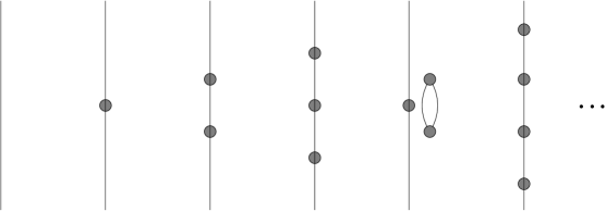
Figure 8: Low-order diagrams for the elementary meson field correlator. The circles represent $\hat{H}_{I}$.

4.2 Effective Interaction for Composite Operators

The above result is now easily transcribed to a system of composite hadrons. In this case the effective correlator (95) becomes

$${\mathfrak{C}}^{(4)}(t,t_{0}) = {\overline{C}^{(4)}(t,t_{0})}^{-1/2}\,{C}^{(4)}(t,t_{0})\,\,{\overline{C}^{(4)}(t,t_{0})}^{-1/2}$$

$$= {\overline{C}^{(4)}(t,t_{0})}^{-1/2}\,{C}_{I}^{(4)}(t,t_{0})\,\,{\overline{C}^{(4)}(t,t_{0})}^{-1/2}+{{\bf 1}}$$

$$\stackrel{{\scriptstyle\rm def}}{{=}} {\mathfrak{C}}_{I}^{(4)}(t,t_{0})+{{\bf 1}}\,,$$

where (54) has been used. This then defines the effective residual interaction

$${\cal H}_{I}\stackrel{{\scriptstyle\rm def}}{{=}}-\lim_{t\rightarrow\infty}\frac{\partial\ln{\mathfrak{C}}^{(4)}(t,t_{0})}{\partial t}\,.$$ (99)

In the lattice simulation the eigenvalues of ${\mathfrak{C}}_{I}^{(4)}(t,t_{0})$ at asymptotic times (within lattice limits) select the low-energy part of the excitation spectrum of the two-body system. This will help to suppress intrinsic excitations of the composite particles and thus yields an effective residual interaction between the mesons (or hadrons) in their respective ground states. How well the excitation of intrinsic degrees of freedom is suppressed depends on the lattice size and on the design of the meson operators.

4.3 Lattice Symmetries

Lattice symmetries should be utilized to reduce the size of the correlation matrices $C^{(2)}$ and $C^{(4)}$. For an $L^{d}\times T$ lattice the action is (usually) invariant under the group $O(d,\mathbb{Z})$ of discrete transformations of the cubic sublattice. The representation theory of these groups is standard [59]. For example, if $d=2$, there are five irreducible representations $\Gamma=A_{1},A_{2},B_{1},B_{2},E$, using a common nomenclature, with dimensionalities $N_{\Gamma}=1,1,1,1,2$ respectively. For $d=3$ there are, again in common nomenclature, $\Gamma=A_{1}^{\pm},A_{2}^{\pm},E^{+},T_{1}^{\pm},T_{2}^{\pm}$ with respective dimensionalities $N_{\Gamma}=1,1,2,3,3$ .

Given a fixed, discrete, lattice momentum $\vec{p}\,^{\prime}$ the application of group transformations $g\in O(d,{\mathbb{Z}})$ generates a set of momenta $\vec{p}={\cal O}_{g}\,\vec{p}\,^{\prime}$ that all have the same length $p=|\vec{p}\,|$. These transformations define a representation of $O(d,{\mathbb{Z}})$ with basis vectors $|\vec{p}>$ which is in general reducible. Let

$$|\vec{p}>=\sum_{\Gamma}\sum_{\epsilon}|(\Gamma,p)\epsilon><(\Gamma,p)\epsilon|\vec{p}>\,,$$ (100)

where $|(\Gamma,p)\epsilon>$ denote a set of basis vectors, $\epsilon=1\ldots$, of the subspace that belongs to $\Gamma$. Those can be constructed with group theoretical techniques [59]. A simple example, which will suffice for our present purposes, is given by choosing $\vec{p}=(p,0)$, assuming $d=2$ and $pL/2\pi\in{\mathbb{N}}$, and the trivial one-dimensional representation $\Gamma=A_{1}$, thus

$$|(A_{1},p)1>=\frac{1}{2}\left(|(+p,0)>+|(0,+p)>+|(-p,0)>+|(0,-p)>\right)\,.$$ (101)

Since both the full and the free correlators $C^{(4)}$ and $\overline{C}^{(4)}$, respectively, commute with all group operations $g\in O(d,{\mathbb{Z}})$ there exist reduced matrices, say $C^{(4;\Gamma)}$ and $\overline{C}^{(4;\Gamma)}$, within each irreducible representation $\Gamma$ such that (Schur’s lemma)

$$<(\Gamma,p)\epsilon|C^{(4)}(t,t_{0})|(\Gamma^{\prime},q)\epsilon^{\prime}>=\delta_{\Gamma\Gamma^{\prime}}\delta_{\epsilon\epsilon^{\prime}}C^{(4;\Gamma)}_{p\,q}(t,t_{0})$$ (102)

and similarly for $\overline{C}^{(4;\Gamma)}$. Above we identify $C_{\vec{p}\,\vec{q}}$ with $<\vec{p}\,|C|\vec{q}>$.

Similar group theoretical considerations are of course also applicable on a coordinate space $|\vec{r}>$ lattice.

An example from the $\mbox{QED}_{2+1}$ model is shown in Fig. 9. The set $\{\overline{W}\}$ of energy levels, with labels $n=1\ldots 6$, belongs to the free system. Those were extracted from the asymptotic time behavior of $\overline{C}^{(4)}_{\vec{p}\,\vec{q}}(t,t_{0})$, see (59), and are degenerate (in general) for momenta of the same magnitude but different directions. The degeneracy is lifted by the residual interaction, the set $\{{W}\}$ being extracted from $C^{(4;\Gamma)}_{p\,q}(t,t_{0})$. Since the angular momentum content of the various representations $\Gamma=A_{1},A_{2},B_{1},B_{2}$ is different ($A_{1}$ mostly contains $\ell=0$, $B_{1}$ and $B_{2}$ contain $\ell=2$, etc) the hyperfine splitting can be attributed to a spin-orbit like force.

Figure 9: Hyperfine splitting due to the residual interaction for the $\mbox{QED}_{2+1}$ model [60]. The labels for $\{W\}$ refer to irreducible representations of the lattice symmetry group $O(2,{\mathbb{Z}})$.

4.4 Truncated Momentum Basis

It is obvious from (59) and (60) that the reduced matrix elements of the free correlator have the form

$$\overline{C}^{(4;\Gamma)}_{p\,q}(t,t_{0})=\delta_{p\,q}\,\left|\bar{c}^{(\Gamma)}_{p}(t,t_{0})\right|^{2}\,.$$ (103)

The functions $\bar{c}^{(\Gamma)}_{p}(t,t_{0})$ are linear combinations of 2-point correlator elements $C^{(2)}_{\vec{p}\,\vec{p}\,^{\prime}}$ with momenta $\vec{p}$ and $\vec{p}\,^{\prime}$ that differ only by their directions.

The eigenvalues of $\overline{C}^{(4;\Gamma)}(t,t_{0})$ describe the time evolution of the eigenstates of a free meson-meson Hamiltonian, say ${\cal H}_{0}$. Since ${\cal H}_{0}$ relates to a composite system, it is useful to think of its degrees of freedom in terms of the relative motion of the two mesons (as clusters) and the intrinsic motion of the individual mesons. Assume, for the purpose of discussion, that the internal excitation energies are large (hard modes) compared to the relative excitation energies (soft modes). In principle, the separation of soft and hard modes may be enforced by choosing a big enough $L^{d}\times T$ lattice:

• Large $L$ will yield a dense momentum spectrum $p\propto L^{-1}$.

• Large $T$ will permit suppression of intrinsic excitations, at large $t$.

In practice there are of course numerical limitations, however, one may check how well those conditions are satisfied. We assume that $\overline{C}^{(4;\Gamma)}$ and $C^{(4;\Gamma)}$ are available on a truncated set of lattice momenta and both have size $N^{(\Gamma)}$. Naturally this will allow us to study features of the effective residual interaction in the long and intermediate range.

The advantage of working in momentum space is that $\overline{C}^{(4;\Gamma)}$ is already diagonal, see (103). Thus the effective correlator (95),(4.2) simply becomes

$${\mathfrak{C}}^{(4;\Gamma)}_{p\,q}(t,t_{0})=\frac{C^{(4;\Gamma)}_{p\,q}(t,t_{0})}{\left|\bar{c}^{(\Gamma)}_{p}(t,t_{0})\right|\left|\bar{c}^{(\Gamma)}_{q}(t,t_{0})\right|}\,.$$ (104)

We envision numerical diagonalization, say

$${\mathfrak{C}}^{(4;\Gamma)}_{p\,q}(t,t_{0})=\sum_{n=1}^{N^{(\Gamma)}}\,v^{(\Gamma)}_{n}(p)\lambda^{(\Gamma)}_{n}(t,t_{0})\,v^{(\Gamma)}_{n}(q)\,.$$ (105)

The eigenvectors $v^{(\Gamma)}_{n}$ are time independent [27], whereas the eigenvalues behave exponentially for asymptotic ($\simeq$) times,

$$\lambda^{(\Gamma)}_{n}(t,t_{0})\simeq a^{(\Gamma)}_{n}\exp(-w^{(\Gamma)}_{n}(t-t_{0}))\,,$$ (106)

or, if periodic boundary conditions across the time extent of the lattice are imposed,

$$\lambda^{(\Gamma)}_{n}(t,t_{0})\simeq c^{(\Gamma)}_{n}\cosh(w^{(\Gamma)}_{n}(t-t_{c}))\,.$$ (107)

Now, extraction of the effective residual interaction as defined in (99) becomes a trivial matter. Provided that the $v^{(\Gamma)}_{n}$ are orthonormal we have

$$<p|{\cal H}_{I}^{(\Gamma)}|q>=\sum_{n=1}^{N^{(\Gamma)}}\,v^{(\Gamma)}_{n}(p)\,w^{(\Gamma)}_{n}\,v^{(\Gamma)}_{n}(q)\,.$$ (108)

These are the desired matrix elements of the effective residual interaction in the truncated momentum basis. They may be used in a variety of ways. For example, in the basis $|\vec{p}>$ of lattice momenta we have

$$<\vec{p}\,|{\cal H}_{I}|\vec{q}>=\sum_{\Gamma}\sum_{\epsilon}<\vec{p}\,|(\Gamma,p)\epsilon><p\,|{\cal H}_{I}^{(\Gamma)}|q><(\Gamma,q)\epsilon|\vec{q}>\,.$$ (109)

This would require computation of the reduced matrix elements for all irreducible representations $\Gamma$ of the cubic lattice symmetry group. However, depending on the system studied, it may well be that $A_{1}$ dominates the series.

The coordinate space matrix elements of the effective residual interaction are obtained from (109) by (discrete lattice) Fourier transformation

$$<\vec{r}\,|{\cal H}_{I}|\vec{s}>=L^{-d}\sum_{\vec{p}}\sum_{\vec{q}}e^{i\vec{p}\cdot(\vec{r}-\vec{s})}e^{-i\vec{q}\cdot(\vec{r}+\vec{s})}<\vec{p}-\vec{q}\,|{\cal H}_{I}|\vec{p}+\vec{q}>\,.$$ (110)

It is useful to write the matrix element of ${\cal H}_{I}$ as a sum of $<-\vec{q}\,|{\cal H}_{I}|+\vec{q}>$ and a remainder. A reference system where the relative momenta before and after a scattering event are $\pm\vec{q}$, respectively, is known as the Breit frame [61]. Then, the sum over $\vec{p}$ in (110) gives rise to $\delta_{\vec{r}\,\vec{s}}$ and thus to a local potential ${\cal V}(\vec{r}\,)$ for the Breit-frame contribution, and a genuinely nonlocal potential ${\cal W}(\vec{r},\vec{s}\,)$ for the remainder

$$<\vec{r}\,|{\cal H}_{I}|\vec{s}>=\delta_{\vec{r}\vec{s}}\,{\cal V}(\vec{r}\,)+{\cal W}(\vec{r},\vec{s}\,)\,.$$ (111)

The potentials are

$${\cal V}(\vec{r}\,)=\sum_{\vec{q}}e^{-i2\vec{q}\cdot\vec{r}}<-\vec{q}\,|{\cal H}_{I}|+\vec{q}>$$ (112)

$${\cal W}(\vec{r},\vec{s}\,) = L^{-d}\sum_{\vec{p}}\sum_{\vec{q}}e^{i\vec{p}\cdot(\vec{r}-\vec{s})}e^{-i\vec{q}\cdot(\vec{r}+\vec{s})}$$ (113)

$$\left(<\vec{p}-\vec{q}\,|{\cal H}_{I}|\vec{p}+\vec{q}>-<-\vec{q}\,|{\cal H}_{I}|+\vec{q}>\right)\,.$$

Results from an actual simulation are displayed in Fig. 10. The (lattice) Fourier transform, see (110), of (109) is shown. An angular momentum projection was employed. Most of the $\ell=0$ partial wave is contained in the $A_{1}$ sector. The corresponding scattering phase shifts, obtained from a Schrödinger equation, are shown in Fig. 11.

Figure 10: Example of a meson-meson potential derived within the momentum-space approach. Local and nonlocal potentials are shown. The model is $\mbox{QED}_{2+1}$ in 2+1 dimensions [60].

Figure 11: Scattering phase shifts, for the $s$-wave, obtained from the effective interaction depicted in Fig. 10. The four data points (filled circles) were computed in Ref. [62], using Lüscher’s method. The same set of phase shifts are also shown modulo $\mbox{180}^{\circ}$ (open circles). The diamonds on the abscissa correspond to the values of $p^{2}=(2\pi/L)^{2}k^{2}$ for an $L=24$ lattice.

4.5 Adiabatic Approximation

Probing the lattice with a set of coordinate space operators of the type

$$\phi_{\vec{x}}(t)=\sum_{\vec{p}}\,e^{-i\vec{p}\cdot\vec{x}}\phi_{\vec{p}}(t)=\bar{\chi}_{d}(\vec{x},t)\,\chi_{u}(\vec{x},t)\,,$$ (114)

where we have used (28), gives us an alternative window on the effective residual interaction. The Fourier transform of the two-meson operator (30) becomes

$$\Phi_{\vec{r}}(t)=\sum_{\vec{p}}\,e^{-i\vec{p}\cdot\vec{r}}\Phi_{\vec{p}}(t)=\sum_{\vec{x}}\sum_{\vec{y}}\delta_{\vec{r},\vec{x}-\vec{y}}\,\phi_{\vec{y}}(t)\,\phi_{\vec{x}}(t)\,.$$ (115)

It corresponds to two composite mesons with relative distance $\vec{r}$ and total momentum zero.

Following Secs. 3.3 and 3.4 we consider the free meson-meson correlator

$$\overline{C}^{(4)}_{\vec{r}\,\vec{s}}(t,t_{0})=\sum_{\vec{p}}\sum_{\vec{q}}\,e^{i\vec{p}\cdot\vec{r}}e^{-i\vec{q}\cdot\vec{s}}\,\,\overline{C}^{(4)}_{\vec{p}\,\vec{q}}(t,t_{0})\,.$$ (116)

It may also be written, using (59), as

$$\overline{C}^{(4)}_{\vec{r}\,\vec{s}}(t,t_{0})=\sum_{\vec{p}}\left(e^{i\vec{p}\cdot(\vec{r}-\vec{s})}+e^{i\vec{p}\cdot(\vec{r}+\vec{s})}\right)|c_{\vec{p}}(t,t_{0})|^{2}\,.$$ (117)

Here $c_{\vec{p}}(t,t_{0})$ is the correlation function of a single-meson interpolating operator with momentum $\vec{p}$, see (57). Its (exponential) time behavior is determined by the total energy $E(p)=\sqrt{m^{2}+p^{2}}$, assuming continuum dispersion for the moment. In the non-relativistic limit, $E(p)\rightarrow m+p^{2}/2m$ as $m\rightarrow\infty$, the correlator thus becomes independent of $\vec{p}$ and may be replaced with $c_{\vec{p}=0}(t,t_{0})$ in (117). This leads to the approximation

$$\overline{C}^{(4)}_{\vec{r}\,\vec{s}}(t,t_{0})\approx L^{2}(\delta_{\vec{r},\vec{s}}+\delta_{\vec{r},-\vec{s}})|c_{\vec{p}=0}(t,t_{0})|^{2}\,.$$ (118)

In coordinate space the free correlator is diagonal in the $m\rightarrow\infty$ limit, whereas in momentum space diagonality is exact.

In terms of the fermion propagator we have, see (57) and (38),(40),

$$c_{\vec{p}=0}(t,t_{0})=\langle L^{-4}\sum_{\vec{x}}\sum_{\vec{y}}|G(\vec{x}t,\vec{y}t_{0})|^{2}\rangle=\langle L^{-2}\sum_{\vec{x}}|G(\vec{x}t,\vec{x}_{0}t_{0})|^{2}\rangle\,.$$ (119)

This is just the time correlation function for a single meson at rest.

Using lattice symmetry, see Secs. 4.3 and 4.4, the reduced correlator matrix has the form

$$\overline{C}^{(4;\Gamma)}_{r\,s}(t,t_{0})\approx\delta_{r,s}|\overline{c}^{(\Gamma)}(t,t_{0})|^{2}\,,$$ (120)

where the asymptotic time behavior is given by

$$\overline{c}^{(\Gamma)}(t,t_{0})\simeq\bar{a}^{(\Gamma)}\,e^{-m(t-t_{0})}\,,$$ (121)

at least for $\Gamma=A_{1}$. The full, interacting, correlator matrix is built from (115)

$$C^{(4)}_{\vec{r}\,\vec{s}}(t,t_{0})=\langle\Phi^{\dagger}_{\vec{r}}(t)\,\Phi_{\vec{s}}(t_{0})\rangle-\langle\Phi^{\dagger}_{\vec{r}}(t)\rangle\langle\Phi^{\phantom{\dagger}}_{\vec{s}}(t_{0})\rangle\,.$$ (122)

Again, the separable term vanishes in our example (flavor assignment). Expressing $C^{(4)}$, via Wick’s theorem, in terms of the fermion propagator and the diagrammatic classification proceeds just like in Secs. 3.3 and 3.4. Alternatively, we may simply Fourier transform (3.3),

$$C^{(4)}_{\vec{r}\,\vec{s}}(t,t_{0}) = L^{-4}\>\sum_{\vec{x}_{1}}\>\sum_{\vec{x}_{2}}\>\sum_{\vec{y}_{1}}\>\sum_{\vec{y}_{2}}\>\delta_{\vec{r},\vec{x}_{1}-\vec{x}_{2}}\delta_{\vec{s},\vec{y}_{2}-\vec{y}_{1}}$$

$$\mbox{}\left\langle\left(\>G^{\ast}(\vec{x}_{2}t,\vec{y}_{2}t_{0})\,G(\vec{x}_{2}t,\vec{y}_{2}t_{0})\,G^{\ast}(\vec{x}_{1}t,\vec{y}_{1}t_{0})\,G(\vec{x}_{1}t,\vec{y}_{1}t_{0})\right.\right.$$

$$\mbox{}+G^{\ast}(\vec{x}_{1}t,\vec{y}_{2}t_{0})\,G(\vec{x}_{1}t,\vec{y}_{2}t_{0})\,G^{\ast}(\vec{x}_{2}t,\vec{y}_{1}t_{0})\,G(\vec{x}_{2}t,\vec{y}_{1}t_{0})$$

$$\mbox{}-G^{\ast}(\vec{x}_{2}t,\vec{y}_{1}t_{0})\,G(\vec{x}_{2}t,\vec{y}_{2}t_{0})\,G^{\ast}(\vec{x}_{1}t,\vec{y}_{2}t_{0})\,G(\vec{x}_{1}t,\vec{y}_{1}t_{0})$$

$$\mbox{}-\left.\left.G(\vec{x}_{2}t,\vec{y}_{1}t_{0})\,G^{\ast}(\vec{x}_{2}t,\vec{y}_{2}t_{0})\,G(\vec{x}_{1}t,\vec{y}_{2}t_{0})\,G^{\ast}(\vec{x}_{1}t,\vec{y}_{1}t_{0})\right)\right\rangle\,.$$

In keeping with the $m\rightarrow\infty$ limit it is reasonable to assume that the relative distance between the (heavy) mesons will not change much during the propagation from $t_{0}$ to $t$. After all, the meson propagation is described by (119). This leads us to neglect the off-diagonal elements of $C^{(4)}$. More precisely, since it costs no energy to change the system according to a transformation that belongs to the lattice symmetry group $O(d,{\mathbb{Z}})$, the correct approximation is

$$C^{(4;\Gamma)}_{r\,s}(t,t_{0})\approx\delta_{r\,s}\,C^{(4;\Gamma)}_{r\,r}(t,t_{0})\,.$$ (124)

Now, the eigenvalues of $C^{(4;\Gamma)}(t,t_{0})$ are just the diagonal elements. Those behave exponentially for asymptotic times.

$$C^{(4;\Gamma)}_{r\,r}(t,t_{0})\simeq a^{(\Gamma)}_{r}\,e^{-W^{(\Gamma)}_{r}(t-t_{0})}\,.$$ (125)

The effective correlator (104) is also diagonal in this approximation

$${\mathfrak{C}}^{(4;\Gamma)}_{r\,s}(t,t_{0})\approx\delta_{r\,s}\,{\mathfrak{C}}^{(4;\Gamma)}_{r\,r}(t,t_{0})\,,$$ (126)

with

$${\mathfrak{C}}^{(4;\Gamma)}_{r\,r}(t,t_{0})\simeq\frac{a^{(\Gamma)}_{r}}{|\bar{a}^{(\Gamma)}|^{2}}e^{-\left[W^{(\Gamma)}_{r}-2m\right](t-t_{0})}\,.$$ (127)

According to our definition (99) the effective residual interaction is

$$<r|{\cal H}_{I}^{(\Gamma)}|s>\approx\delta_{r\,s}{\cal V}^{(\Gamma)}(r)\,,\quad\mbox{with}\quad{\cal V}^{(\Gamma)}(r)=W^{(\Gamma)}_{r}-2m\,.$$ (128)

The above line of arguments is somewhat similar in spirit to the Born-Oppenheimer approximation often used with systems of two atoms or molecules [63]. The time scale for the dynamics of the interaction is much faster than the time scale for the dynamics of the motion for the atoms. Borrowing a thermodynamics term, we speak of an adiabatic approximation. In our case we simply compute the total energy of the two-meson system at fixed (static) relative distance $r$ and interpret the difference to the ground state energy as a potential [64].

An example from numerical work on the $\mbox{QED}_{2+1}$ model [65] is shown in Fig. 12. The left part displays the static potential ${\cal V}^{(\Gamma)}$ according to (128). The distance $\vec{r}=0$ is forbidden by the Pauli exclusion principle. This is the reason for the increase (repulsive core) of the potential as $r\rightarrow 0$.

Figure 12: Static meson-meson potential for the $\mbox{QED}_{2+1}$ model according to (128), on the left. On the right a somewhat different approximation according to (129) serves to check the perturbative definition of ${\cal H}_{I}$.

The right part of Fig. 12 shows a potential computed slightly differently, for the sake of comparison. The perturbative version of (127) leads to

$${\cal V}^{(\Gamma)}(r)\approx\frac{1}{t-t_{0}}\left[1-\frac{{\mathfrak{C}}^{(4;\Gamma)}_{r\,r}(t,t_{0})}{a^{(\Gamma)}_{r}|\bar{a}^{(\Gamma)}|^{-2}}\right]\,.$$ (129)

In this way the $r$-dependence of $a^{(\Gamma)}_{r}$ enters the analysis. The results in Fig. 12 are similar. They shed some light on the validity of the perturbative definition of ${\cal H}_{I}$ put forward in Sec. 4.1.

Of course, only the local part of the effective residual interaction is accessible in this way. Note, however, that a local potential

$${\cal V}(\vec{r}\,)=\sum_{\Gamma}\sum_{\epsilon}<\vec{r}\,|(\Gamma,r)\epsilon>{\cal V}^{(\Gamma)}(r)<(\Gamma,r)\epsilon|\vec{r}>\,,$$ (130)

compared to (109), may not be the same as the approximate local potential of (112) even if the untruncated correlation matrices are used. The reason is that diagonal elements of the non-local part of the effective residual interaction may contribute to the adiabatic local potential.

The adiabatic approximation hinges on the assumption of heavy ($m\rightarrow\infty$) partners. This should be reasonable if at least one of the quarks in each hadron is heavy, say an s-quark. However, in the chiral limit ($m_{\pi}\rightarrow 0$), using Wilson fermions, the adiabatic approximation is expected to fail if pseudoscalar mesons are involved. In this case momentum space methods like in Sec. 4.4 are preferable. Finally, the quality of the adiabatic approximation can of course be tested numerically by computing off-diagonal elements of the correlation matrices.

4.6 Analysis on a Periodic Lattice

Periodic boundary conditions across the space extent of the lattice are a common choice. The potentials ${\cal V}(\vec{r}\,)$ and ${\cal W}(\vec{r},\vec{s}\,)$, see (112) and (113), extracted from the lattice simulation, in one or the other way, will reflect those conditions. In particular, the maximal usable relative distance $r$ is $L/2$.

Suppose it is desired to make a fit to the lattice local potential with a class of functions $V^{(\alpha)}(\vec{r}\,)$ depending on a set of parameters $\alpha$. An example is

$$V^{(\alpha)}(\vec{r}\,)=\alpha_{1}\frac{1-\alpha_{2}r^{\alpha_{5}}}{1+\alpha_{3}r^{\alpha_{5}+1}e^{\alpha_{4}r}}+\alpha_{0}\,.$$ (131)

This class (see Fig. 13) has enough flexibility to match heuristic features of the hadronic interaction, like short-range repulsion or attraction as the case may be, and a long range Yukawa form

$$V^{(\alpha)}(\vec{r}\,)\rightarrow-\frac{\alpha_{1}\alpha_{2}}{\alpha_{3}}\frac{e^{-\alpha_{4}r}}{r}+\alpha_{0}\quad\mbox{as}\quad r\rightarrow\infty\,.$$ (132)

The periodic extension, defined as

$$V^{(\alpha)}_{L}(\vec{r}\,)=\sum_{\vec{n}}V^{(\alpha)}(\vec{r}-\vec{n}L)\,,$$ (133)

where $\vec{n}$ are vectors with $d$ whole number components, can then be used to fit the lattice potentials with

$$\chi^{2}(\alpha)=\frac{1}{N}\sum_{\vec{r}}|{\cal V}(\vec{r}\,)-V^{(\alpha)}_{L}(\vec{r}\,)|^{2}\frac{1}{\sigma^{2}(\vec{r}\,)}\,.$$ (134)

Here the sum runs over the set of $N$ lattice distances $\vec{r}$ for which ${\cal V}(\vec{r}\,)$ has been computed.

Figure 13: Example of $V^{(\alpha)}$ as defined in (131). The parameters $\alpha$ are arbitrarily chosen, for the purpuse of illustration.

The idea behind using a periodic extension, like (133), is to account for the fact that the lattice hadrons are interacting with their replicas in adjacent copies of the periodic lattice. With $\chi^{2}$ minimized, we would take $V^{(\alpha)}(\vec{r}\,)$ and $W^{(\beta)}(\vec{r},\vec{s}\,)$ obtained from a similar fit, as the results of the simulation.

5 Current State in QCD in 3+1 Dimensions

At the time of this writing, lattice work on the subject of hadronic interaction is in an exploratory phase. Nevertheless, it is useful to convey what has been done through some selected examples. We will not include in this section results other than $\mbox{QCD}_{3+1}$, for example $O(4)$ symmetric field theories and four-fermion models [66, 67, 68], models exploring static quark geometry [69, 70], studies with an SU(2) gauge group [71], and work using the hamiltonian lattice formulation [72].

5.1 Scattering Lengths for $\pi$ and N Systems

To date the most elaborate application within $\mbox{QCD}_{3+1}$ has been via Lüscher’s formula (9) by the CP-PACS collaboration aiming at scattering lengths for the $\pi$–$\pi$, $\pi$–N, K–N, $\bar{\rm K}$–N, and N–N systems [19, 18, 20, 21, 22, 23, 24, 25, 26]. The collaboration has applied considerable resources to this problem, recently using lattices as large as $L^{3}\times T=32^{3}\times 60$ [24]. However, for most of their earlier explorations [21] lattices typically of size $12^{3}\times 20$ with lattice lattice constants in the range of $a\approx 0.15$ – $0.30$ fm were used.

Extracting the s-wave scattering length $a_{0}$ from Lüscher’s formula

$$W_{h_{1}h_{2}}-(m_{h_{1}}+m_{h_{2}})=-\frac{2\pi(m_{h_{1}}+m_{h_{2}})a_{0}}{m_{h_{1}}m_{h_{2}}L^{3}}[1+c_{1}\frac{a_{0}}{L}+c_{2}(\frac{a_{0}}{L})^{2}+o(L^{-3})]\,,$$ (135)

where $h_{1}$ and $h_{2}$ denote hadrons 1 and 2, see (9), requires a standard mass calculation on the lattice. One therefore needs to compute correlation functions of suitable operators, say $\phi_{h_{1}}(t)$ and $\phi_{h_{2}}(t)$. For illustration, some examples using Wilson fermions are

$$\phi_{\pi^{+}}(t) = -\sum_{\vec{x}}\bar{\psi}_{dA}(\vec{x},t)\gamma_{5}{\psi}_{uA}(\vec{x},t)$$ (136)

$$\phi_{\pi^{0}}(t) = \frac{1}{\sqrt{2}}\sum_{\vec{x}}\left(\bar{\psi}_{uA}(\vec{x},t)\gamma_{5}{\psi}_{uA}(\vec{x},t)-\bar{\psi}_{dA}(\vec{x},t)\gamma_{5}{\psi}_{dA}(\vec{x},t)\right)\rule{25.83325pt}{0.0pt}$$ (137)

$$\phi_{K^{+}}(t) = \sum_{\vec{x}}\bar{\psi}_{sA}(\vec{x},t)\gamma_{5}{\psi}_{uA}(\vec{x},t)\,,$$ (138)

etc, where $A=1,2,3$ represents SU(3) color. Only zero-momentum interpolating fields are needed here. Kogut-Susskind, or staggered, fermions [47, 48, 49] were also used by the CP-PACS collaboration. The construction of operators with specific hadron quantum numbers is technically more complicated, however [73]. The authors of Ref. [21] chose to construct correlation functions where sources and sinks between $h_{1}$ and $h_{2}$ are one time slice apart. For the one-hadron systems this means

$$C_{h_{1}}(t,0) = \langle\phi_{h_{1}}(t)\phi^{\dagger}_{h_{1}}(0)\rangle-\langle\phi_{h_{1}}(t)\rangle\langle\phi^{\dagger}_{h_{1}}(0)\rangle$$

$$\simeq \bar{a}_{h_{1}}e^{-m_{h_{1}}t}$$

$$C_{h_{2}}(t+1,1) = \langle\phi_{h_{2}}(t+1)\phi^{\dagger}_{h_{2}}(1)\rangle-\langle\phi_{h_{2}}(t+1)\rangle\langle\phi^{\dagger}_{h_{2}}(1)\rangle$$

$$\simeq \bar{a}_{h_{2}}e^{-m_{h_{2}}t}\,,$$

where $\simeq$ indicates the asymptotic behavior. The two-hadron interpolating fields are constructed from linear combinations of products of one-hadron operators, respecting the one-time-slice offset. Denoting those by $\Phi_{h_{1}h_{2}}(t,t+1)$ illustrational examples in the $\pi$–$\pi$ system with isospin $I$ are

$$\Phi_{\pi\pi}^{(I=0,I_{3}=0)}(t,t+1) = \frac{1}{\sqrt{3}}\left(\phi_{\pi^{+}}(t)\phi_{\pi^{-}}(t+1)\right.$$

$$\left.-\phi_{\pi^{0}}(t)\phi_{\pi^{0}}(t+1)+\phi_{\pi^{-}}(t)\phi_{\pi^{+}}(t+1)\right)$$

$$\Phi_{\pi\pi}^{(I=2,I_{3}=2)}(t,t+1) = \phi_{\pi^{+}}(t)\phi_{\pi^{+}}(t+1)\,.$$ (142)

In the s-wave $I=1$ is not allowed (Bose symmetry). The corresponding two-hadron system correlator is

$$C_{h_{1}h_{2}}(t+1,t,1,0)=$$

$$\langle\Phi_{h_{1}h_{2}}(t,t+1)\Phi^{\dagger}_{h_{1}h_{2}}(0,1)\rangle-\langle\Phi_{h_{1}h_{2}}(t,t+1)\rangle\langle\Phi^{\dagger}_{h_{1}h_{2}}(0,1)\rangle\,.$$

The measurement of the s-wave scattering length $a_{0}$ via Lüscher’s formula (135) requires the energy difference $W_{h_{1}h_{2}}-(m_{h_{1}}+m_{h_{2}})$, which can be extracted from the asymptotic time behavior of the ratio of correlation functions

$$R(t)\stackrel{{\scriptstyle\rm def}}{{=}}\frac{C_{h_{1}h_{2}}(t+1,t,1,0)}{C_{h_{1}}(t,0)C_{h_{2}}(t+1,1)}\simeq\frac{a_{h_{1}h_{2}}}{\bar{a}_{h_{1}}\bar{a}_{h_{2}}}e^{-(W_{h_{1}h_{2}}-(m_{h_{1}}+m_{h_{2}}))t}\,.$$ (144)

Baryon interpolating field operators are more complicated. For the proton ($N^{+}$) and neutron ($N^{0}$) standard choices for zero-momentum operators are

$$\phi_{N^{+}}(t) = \sum_{\vec{x}}\epsilon_{ABC}\left[\left(\bar{\psi}_{uA}^{T}(\vec{x},t)\tilde{\cal C}\psi_{dB}(\vec{x},t)\right)\psi_{uB}(\vec{x},t)\right.$$ (145)

$$\phantom{xxxxxxxx}\left.-\left(\bar{\psi}_{dA}^{T}(\vec{x},t)\tilde{\cal C}\psi_{uB}(\vec{x},t)\right)\psi_{uB}(\vec{x},t)\right]$$

$$\phi_{N^{0}}(t) = \sum_{\vec{x}}\epsilon_{ABC}\left[\left(\bar{\psi}_{uA}^{T}(\vec{x},t)\tilde{\cal C}\psi_{dB}(\vec{x},t)\right)\psi_{dB}(\vec{x},t)\right.$$ (146)

$$\phantom{xxxxxxxx}\left.-\left(\bar{\psi}_{dA}^{T}(\vec{x},t)\tilde{\cal C}\psi_{uB}(\vec{x},t)\right)\psi_{dB}(\vec{x},t)\right]\,,$$

where $\tilde{\cal C}$ means charge conjugation and $A,B,C$ are color indices. Operators for the ${}^{3}S_{1}$ and ${}^{1}S_{0}$ channels of the N–N system are constructed in Ref. [21]

$$\Phi_{{}^{3}S_{1}}(t,t+1) = \frac{1}{\sqrt{2}}\left(\phi_{N^{+}}(t)\phi_{N^{0}}(t+1)-\phi_{N^{0}}(t)\phi_{N^{+}}(t+1)\right)\rule{25.83325pt}{0.0pt}$$ (147)

$$\Phi_{{}^{1}S_{0}}(t,t+1) = \phi_{N^{+}}(t)\phi_{N^{+}}(t+1)\,.$$ (148)

Again, ratios like (144) allow the extraction of the desired mass shifts.

Computation of the above time correlation functions requires matrix elements of the quark propagator $G=D^{-1}$, where $D(x,y)$ denotes the Dirac, or fermion, matrix and $x=(\vec{x},t)$, are space-time lattice sites. Since a complete solution of

$$\sum_{x{{}^{\prime\prime}}}D(x{{}^{\prime}},x{{}^{\prime\prime}})\,G(x{{}^{\prime\prime}},x)={\bf 1}\,\delta_{x{{}^{\prime}},x}\,,$$ (149)

where ${\bf 1}$ means the unit matrix in color-Dirac space, is not feasible in practice source techniques are typically used to obtain at least some columns of $G$. The CP-PACS collaboration has employed so called wall sources. These are defined by placing a point source of value ${\bf 1}$ on each spatial site of a certain time slice $t$, specifically

$$\sum_{\vec{x}{{}^{\prime\prime}}t^{\prime\prime}}D(\vec{x}{{}^{\prime}}t^{\prime},\vec{x}{{}^{\prime\prime}}t^{\prime\prime})\,G_{t}(\vec{x}{{}^{\prime\prime}}t^{\prime\prime})={\bf 1}\,\sum_{\vec{x}}\delta_{(\vec{x}{{}^{\prime}}t^{\prime}),(\vec{x}t)}={\bf 1}\,\delta_{t^{\prime}t}\,.$$ (150)

Note that the uniform nature of the wall source implies that the solution vector $G_{t}$ must be independent of $\vec{x}{{}^{\prime}}$. Indeed, employing (149) it is obvious that

$$G_{t}(\vec{x}{{}^{\prime\prime}}t^{\prime\prime})=\sum_{\vec{x}}\,G(\vec{x}{{}^{\prime\prime}}t^{\prime\prime},\vec{x}t)\,.$$ (151)

Loosely speaking, since the spatial source is structureless quark propagation to $x{{}^{\prime\prime}}$ proceeds in ‘the same way’ regardless of the spatial point of origin. However, this is not a gauge invariant mechanism. Under a gauge transformation $D(x,y)=U^{\dagger}(x)\tilde{D}(x,y)U(y)$, etc, the wall source becomes ${\bf 1}U(\vec{x}{{}^{\prime}}t^{\prime})\,\delta_{t^{\prime},t}$. Thus, in contrast to $G(\vec{x}{{}^{\prime\prime}}t^{\prime\prime},\vec{x}t)$, the (numerical) solution $G_{t}(\vec{x}{{}^{\prime\prime}}t^{\prime\prime})$ of (150) does not transform covariantly. Gauge dependent noise in hadronic correlation functions caused by the wall sources is specifically created at time slices where two wall sources or one wall source and one sink are placed. This can be seen from Fig. 14 which shows a diagramatic analysis of the correlators for the $\pi$–$\pi$, $\pi$–N, and N–N systems in terms of quark propagators and the corresponding wall sources and sinks.

Figure 14: Diagrams contributing to hadron-hadron 4-point functions, from Ref. [21]. Arrowed lines represent quark or antiquark propagators. Wall sources are depicted by short bars, and circles represent sinks for hadron operators. The diagrams in (i), (ii), and (iii) are for the $\pi$–$\pi$, $\pi$–N, and N–N systems, respectively. The decompositions (153) and (154), for example, refer to the labels D,C,R,V of diagrams (i).

Wall sources are depicted as short lines and sinks as circles. The time slices refer to $t_{1}=0,t_{2}=1,t_{3}=t,t_{4}=t+1$. For example the $\pi$–$\pi$ rectangular diagram in Fig. 14(i) corresponds to

$$C^{R}(t_{4},t_{3},t_{2},t_{1})=\sum_{\vec{x}_{2},\vec{x}_{3}}\langle{\rm Re}{\rm Tr}[G^{\dagger}_{t_{1}}(\vec{x}_{2}t_{2})G_{t_{4}}(\vec{x}_{2}t_{2})G^{\dagger}_{t_{4}}(\vec{x}_{3}t_{3})G_{t_{1}}(\vec{x}_{3}t_{3})]\rangle\,.$$ (152)

The paths involved in the computation of $C^{R}$ are not all closed, they are interupted at time slices where a (nonlocal) wall source meets a (local) sink, or two wall sources meet. This happens, for example, at $t_{1}$ and $t_{4}$, see (152) and Fig. 14.

In order to deal with the gauge noise problem two strategies may be employed: The first one is gauge fixing, the other one is to rely on gauge fluctuations to cancel out in the final correlation function. For the latter the gauge noise is expected to decrease as $\sim L^{3/2}$ for sufficiently large $L$ [21].

Correlator ratios (144) for various channels can be expressed in terms of linear combinations of certain diagrams which are referred to by labels D, C, R, V, etc, in Fig. 14. For example, in the Wilson fermion scheme

$$R^{\pi\pi}_{I=0}(t) = R^{D}(t)+\frac{1}{2}R^{C}(t)-3R^{R}(t)+\frac{3}{2}R^{V}(t)$$ (153)

$$R^{\pi\pi}_{I=2}(t) = R^{D}(t)-R^{C}(t)\,.$$ (154)

For staggered fermions the corresponding decomposition is slightly different.

Typical results for a ratio function (144) are shown in Fig. 15 for the $I=0$ and $I=2$ channels of the $\pi$–$\pi$ system.

Figure 15: Ratios (153) and (154) for the $\pi$–$\pi$ four-point function, from Ref. [21]. This example is for Wilson fermions at $\beta=5.7$, $\kappa=0.164$, and wall sources without gauge fixing. The lattice size is $12^{3}\times 20$.

A selection of scattering lengths, again for the $\pi$–$\pi$ system, is displayed in Fig. 16.

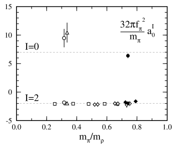
Figure 16: Comparison of various scattering length results in the $I=0$ and $I=2$ channels for the $\pi$–$\pi$ system, with units as given in the picture. Solid and open plot symbols refer to Wilson and Kogut-Sussking fermions, respectively. Results are from Ref. [21], except for the squares and diamonds, which are from Refs. [16, 17]. Dotted lines are current algebra predictions.

In Fig. 17 a comparison of scattering lengths for the systems $\pi$–$\pi$, $\pi$–N, and N–N is made.

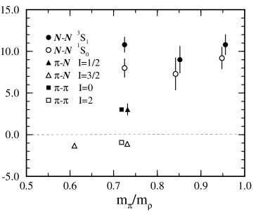
Figure 17: Comparison of scattering lengths for the $\pi$–$\pi$, $\pi$–N, and N–N systems in physical units $a_{0}$ [fm] versus the $\pi$–$\rho$ mass ratio. These are (quenched) results for Wilson fermions from Ref. [21] at lattice constant $a=0.137(2)~{}{\rm fm}$.

Table 1 contains the main results of the lattice simulation and current algebra predictions. A chiral extrapolation has not been made in [21]. Thus, perhaps not surprisingly, the lattice results agree best with the current algebra predictions that use the hadron masses supplied by the actual lattice simulation. The N–N system is special because of its large size. Realistic lattice results for the scattering length cannot be expected with contemporary resources.

Table 1: Selected results from Ref. [21]. Scattering lengths $a_{0}$ for the s-wave in various channels are shown in physical units [fm], for the lattice (lat), experiment (exp), and current algebra (cua). The lattice results are for Wilson fermions on a $12^{3}\times 20$ lattice with $\beta=5.7$. Light-quark masses are large as indicated by $m_{\pi}/m_{\rho}=0.74$ and $m_{N}/m_{\rho}=1.57$. Experimental and current algebra results are compiled from Refs. [74, 75] and [76], respectively. In the last column the masses from the lattice simulation enter the current algebra predictions.

		lat	exp	cua	cua(lat)
$\pi$–$\pi$	$I=0$	$+3.02(17)$	$+0.37(7)$	$+0.222$	$+3.47(5)$
	$I=2$	$-0.924(40)$	$-0.040(17)$	$-0.0635$	$-0.993(16)$
$\pi$–N	$I=1/2$	$+3.04(66)$	$+0.245(4)$	$+0.221$	$+2.701(41)$
	$I=3/2$	$-1.10(20)$	$-0.143(6)$	$-0.111$	$-1.350(20)$
N–N	${}^{3}S_{1}$	$+10.8(9)$	$-5.432(5)$
	${}^{1}S_{0}$	$+8.0(1.1)$	$+20.1(4)$
K–N	$I=0$	$+0.55(47)$	$-0.0075$	$\phantom{-}0$	$\phantom{-}0$
	$I=1$	$-1.56(13)$	$-0.225$	$-0.399$	$-2.701(41)$
$\bar{\mbox{K}}$–N	$I=0$	$+4.64(37)$	$-1.16+i\,0.49$	$+0.598$	$+4.051(61)$
	$I=1$	$+2.63(64)$	$+0.17+i\,0.41$	$+0.199$	$+1.350(20)$

5.2 Static $N-N$ and $N-{\bar{N}}$ Potentials

Beyond the zero-momentum limit (scattering lengths) systems of hadrons with at least one heavy quark each pose the least technical difficulties. Going to the extreme, an infinitely heavy quark may be interpreted as a static color source. This idea goes back to Wilson’s original work [37] and played a role in demonstrating confinement.

The time evolution operator of a static color source (a quark) located at fixed $\vec{x}$ is given by the product of link variables $U_{4}(\vec{x}t)\in SU(3)$ along a line $t_{i}\rightarrow t_{i}+1\rightarrow\ldots\rightarrow t_{f}$ in the time direction, $\mu=4$. For a lattice $L^{3}\times T$ with periodic boundary conditions in the time direction the line is closed, $t_{i}=t_{f}$. The trace of such an operator

$$Q(\vec{x})=\frac{1}{3}\mbox{Tr}\prod_{t=1}^{T}U_{4}(\vec{x}t)$$ (155)

is gauge invariant and is known as a Polyakov loop. It represents a static quark at $\vec{x}$, and $Q^{\dagger}(\vec{x})$ represents a static antiquark at $\vec{x}$. In the finite-temperature formalism the expectation value [78, 79, 64]

$$L^{-3}\sum_{\vec{x}}\langle Q(\vec{r}+\vec{x})Q^{\dagger}(\vec{x})\rangle=e^{-T\,F_{Q\overline{Q}}(\vec{r}\,)}$$ (156)

is related to the free energy $F_{Q\overline{Q}}(\vec{r}\,)$, loosely (but imprecisely) referred to as the heavy quark-antiquark potential. Adopting this interpretation it is interesting to compute the free energies of two clusters of two or three quarks [80, 81, 82]. Consider

$$O(\vec{x})=\sum_{\vec{y}_{1}\vec{y}_{2}\vec{y}_{3}}\rho(\vec{y}_{1}\vec{y}_{2}\vec{y}_{3})Q(\vec{x}+\vec{y}_{1})Q(\vec{x}+\vec{y}_{2})Q(\vec{x}+\vec{y}_{3})\,,$$ (157)

where $\rho$ is some function symmetric in $\vec{y}_{1}\vec{y}_{2}\vec{y}_{3}$, for example a Gaussian or the characteristic function of a sphere with radius $R$, which serves as an ad-hoc model for the three-quark cluster. The free energy of two three-quark clusters at separation $\vec{r}$ then is

$$F(\vec{r}\,)=-\frac{1}{T}\ln L^{-3}\sum_{\vec{x}}\langle O(\vec{r}+\vec{x})O(\vec{x})\rangle\,.$$ (158)

An example of $F(\vec{r}\,)$ can be seen in Fig. 18. There is attraction in the overlap region of the clusters, somewhat reflecting the shape of $\rho$. The cluster interaction possesses no dynamics in this construction.

Figure 18: Interaction energies of hadron-hadron systems versus the relative distance [80, 81] in the finite-temperature formalism. Hadronic structure is represented by a static cluster. The radius of the cluster is $R=2$ in lattice units.

5.3 Heavy-Light Meson-Meson Systems

A step towards a more realistic calculation is to make some of the quarks dynamical. In a system of two mesons which consist of a heavy and a light quark each, we may still approximate the heavy quark by a Polyakov loop, as above. The role of the static quarks then is to localize the mesons. This situation suggests using the coordinate-space approach of Sec. 4.5.

Thus we take, say in the staggered scheme,

$$\phi_{\vec{x}}(t)=\bar{\chi}_{h}(\vec{x},t)\,\chi_{u}(\vec{x},t)\,,$$ (159)

where $h$ is the heavy flavor ($h=s,c,\ldots$). The two-meson interpolating field is defined just like (115). However, the heavy-flavor propagator, $G^{(h)}$, is taken in the limit $m_{h}\rightarrow\infty$. This is achieved by using the hopping parameter expansion [83, 77] and keeping the leading term only. We thus use

$$G^{(h)}(\vec{x}t,\vec{y}t_{0})=\delta_{\vec{x},\vec{y}}\,[\frac{1}{2m_{h}}(-1)^{x_{1}+x_{2}+x_{3}}]^{t-t_{0}}\prod_{\tau=1}^{t-t_{0}}\,U_{4}(\vec{x}\tau)\,.$$ (160)

The product of link variables becomes proportional to the Polyakov loop (155) for $t-t_{0}=T$. With $G^{(h)}$ diagonal in the space sites the 2-point and 4-point correlators become

$$C^{(2)}(t,t_{0}) = \langle L^{-6}\sum_{\vec{x}}G^{(h)\ast}_{BA}(\vec{x}t,\vec{x}t_{0})\,G_{BA}(\vec{x}t,\vec{x}t_{0})\rangle$$ (161)

$$C^{(4)}_{\vec{r}}(t,t_{0}) = \langle L^{-12}\sum_{\vec{x}}[G^{(h)\ast}_{BA}(\vec{x}t,\vec{x}t_{0})\,G_{BA}(\vec{x}t,\vec{x}t_{0})$$

$$\rule{31.43047pt}{0.0pt}\times G^{(h)\ast}_{DC}(\vec{x}-\vec{r}\,t,\vec{x}-\vec{r}\,t_{0})\,G_{DC}(\vec{x}-\vec{r}\,t,\vec{x}-\vec{r}\,t_{0})$$

$$\rule{31.43047pt}{0.0pt}-G^{(h)\ast}_{BA}(\vec{x}t,\vec{x}t_{0})\,G_{BC}(\vec{x}-\vec{r}\,t,\vec{x}t_{0})$$

$$\rule{31.43047pt}{0.0pt}\times G^{(h)\ast}_{DC}(\vec{x}-\vec{r}\,t,\vec{x}-\vec{r}\,t_{0})\,G_{DA}(\vec{x}t,\vec{x}-\vec{r}\,t_{0})]\rangle\,.$$

Sums over color indices $A,B,C,D$ are understood. The 4-point correlator (5.3) is a sum of two terms which are illustrated in Fig. 19. The light quarks can be exchanged between the mesons. Thus, besides gluon effects, also quark dynamics is included in the effective residual interaction.

Figure 19: Diagrams for the heavy-light meson-meson system. The thick and thin lines represent propagators for the heavy (static) and the light (dynamical) quark, respectively.

For distances $\vec{r}\neq 0$ parallel to the coordinate axes, the $A_{1}$ sector projection, see Sec. 4.3, is similar to (101), thus

$$C^{(4;A_{1})}_{r}(t,t_{0})=\frac{1}{4}\sum_{\vec{r},|\vec{r}|=r}C^{(4)}_{\vec{r}}(t,t_{0})\,.$$ (163)

According to (127) the effective correlator

$${\mathfrak{C}}^{(4;A_{1})}_{r\,r}(t,t_{0})\approx\frac{C^{(4;A_{1})}_{r}(t,t_{0})}{|C^{(2)}(t,t_{0})|^{2}}\simeq c_{r}\,e^{-V^{(A_{1})}(r)(t-t_{0})}$$ (164)

serves to extract the (adiabatic) potential $V^{(A_{1})}(r)$. Examples from an actual simulation [33] are shown in Fig. 20.

Figure 20: Meson-meson energies $W(r)=V^{(A_{1})}(r)$, see (164), for several light-quark masses of staggered fermions. Energies at distance $r/a=3$ are degenerate, $|\vec{r}|=|(2,2,1)|=(3,0,0)|$. Those data points are slightly shifted [84].

In the simple case of a one-hadron local operator it is possible to express the corresponding time correlation function in terms of propagator matrix elements from a source located at only one fixed lattice site, say $x=(\vec{x}_{0}t_{0})$. This is done by using translational invariance of the lattice action in the manner outlined in Sec. 3.2 leading to (40), for example. The cost of computing this is greatly reduced because only one column $G(\vec{x}t,\vec{x}_{0}t_{0})$ of the inverse fermion matrix (per color-Dirac index) is needed. In the case of a two-hadron system translational invariance might still be utilized to replace some propagator elements with $G(\vec{x}t,\vec{x}_{0}t_{0})$, for example via $\vec{x}_{1}\rightarrow\vec{x}_{1}+\vec{y}_{1}-\vec{x}_{0}$ in (3.3). In the latter case elements $G(\vec{x}t,\vec{y}t_{0})$ where $\vec{x}$ and $\vec{y}$ run separately over all spatial lattice sites still remain. Those are known as all-to-all propagators. Their computation poses an almost unavoidable problem in multi-hadron systems. The wall sources defined through (150) seemingly circumvent this difficulty, however, only at the cost of violating gauge invariance of the correlation functions, see Sec. 5.1. In a heavy-light hadron-hadron system, like (5.3) for example, the needed minimum number of sources is the number of relative spatial distances distances $\vec{r}$ that are probed (including those related by $O(3,\mathbb{Z})$ symmetry).

The use of stochastic methods for dealing with the all-to-all propagator problem was already discussed in some detail. Even in cases where translational invariance can be utilized it may be advantageous to employ random sources instead. The reason is that the additional (large) sums over lattice sites work to reduce statistical errors in the correlation functions. Besides, it may also be the only computationally viable strategy. In a typical application a random source is chosen to be nonzero on one time slice only, say $t_{0}$, as in (65) and (66). In this case propagation from any lattice site to any other lattice site within the same time slice is computed using the stochastic estimator, whereas propagation between lattice sites with different times, such as $t$ and $t_{0}$, is computed with machine precision. An important consequence is that the errors for propagation in space and time directions are different. While the latter is as small as the matrix inversion algorithm permits (e.g. a conjugate gradient) the former is limited by the variance of the random source probability distribution and, in particular, is independent of the distance between the lattice sites. This is a serious drawback, it means that stochastic estimation is futile in computing the usual (hadronic) time correlation functions since their exponentially decreasing signal would be concealed by the essentially constant error of the stochastic estimator.

This problem can be dealt with to some extent by a method called maximum variance reduction [85], see also [86, 87]. The idea is to enclose disjoint regions of lattice sites by fixed-source boundaries in order to increase sample sizes. One such region may consist of a single point [88]. Another, somewhat related, example is $R=\{(\vec{x},t_{0})|\vec{x}\in L^{3}\}$, i.e. the spatial volume at time slice $t_{0}$. An estimator for propagation between any two points in disjoint regions is then variance reduced. Specifically, starting from

$$Z=\int[d\phi\,d\phi^{\ast}]\exp(-\frac{1}{2}\phi^{\dagger}A\phi)\,,$$ (165)

where $\phi$ is an auxiliary scalar complex lattice field and $A$ is a hermitean positive definite matrix, one may generate stochastically independent ensembles of fields $\{\phi\}$ by way of common Monte Carlo methods with the gaussian probability distribution implied in (165). Writing $i=C\mu x$, etc, for the color-Dirac-site indices it is then straightforward to show that

$$A_{ij}^{-1}=\frac{1}{Z}\int[d\phi\,d\phi^{\ast}]\exp(-\frac{1}{2}\phi^{\dagger}A\phi)\,\phi_{j}^{\ast}\phi_{i}\cong\langle\phi_{j}^{\ast}\phi_{i}\rangle\,,$$ (166)

where in this context $\langle\ldots\rangle$ means the average over the ensemble $\{\phi\}$. The above equations become useful for the choice

$$A=Q^{\dagger}Q\,,$$ (167)

with $Q=Q[U]$ being the fermion matrix for a given gauge field configuration $U$. In the Wilson scheme, for example, it has the form $Q[U]={\bf 1}-\kappa D[U]$. Quark propagator elements $G_{ij}$ can then be estimated from the ensemble averages

$$G_{ij}\stackrel{{\scriptstyle\rm def}}{{=}}Q_{ij}^{-1}\cong\langle(Q\phi)^{\ast}_{j}\,\phi_{i}\rangle\,.$$ (168)

If the variance of the above estimator is $\sigma_{ij}$ the statistical error is $\sigma_{ij}/\sqrt{N_{\phi}}$ for an ensemble of size $N_{\phi}$. However, the crucial point here is that the variance $\sigma_{ij}$, for $i=C\mu x$ and $j=B\nu y$, is essentially independent of the space-time distance $|x-y|$, say $\sigma_{ij}\approx\sigma$ while $\sigma$ is of the order of one inherited from its gaussian ancestry. This effect spoils using the stochastic estimator for the purpose of computing exponentially decreasing time correlation functions.

To alleviate the problem the authors of Ref. [85] proceed to consider a subset, or region, of contiguous lattice sites. Describe this region by sets of sites $R$ and $S$, with $R\cap S=\emptyset$, where $R$ contains all entirely interior points (having 8 neighbors $\in R\cup S$) and $S$ is the boundary (having 1 through 7 neighbors $\in R\cup S$). In the process of generating ensembles $\{\phi\}$ from (165), consider a certain field $\phi$. Then, the field conponents on the boundary $S$ are kept fixed

$$s_{l}\stackrel{{\scriptstyle\rm def}}{{=}}\phi_{l}\quad{\rm for}\quad l\in S\,,$$ (169)

and instead of (165) one uses

$${\cal Z}=\int_{R}[d\phi\,d\phi^{\ast}]\exp\left(-\frac{1}{2}(\phi^{\dagger}_{i}\bar{A}_{ij}\phi_{j}+\phi^{\dagger}_{i}\tilde{A}_{il}s_{l}+s^{\dagger}_{l}\tilde{A}_{lj}\phi_{j})\right)\,,$$ (170)

where $i,j\in R$ and $l\in S$ is understood for the index sum ranges and the notations $\bar{A}$ and $\tilde{A}$ are introduced for the corresponding blocks of $A$. The integral runs over the field components located on $R$. Now the $R$-averaged random source field

$$v_{k}=\frac{1}{\cal Z}\int_{R}[d\phi\,d\phi^{\ast}]\exp\left(-\frac{1}{2}(\phi^{\dagger}_{i}\bar{A}_{ij}\phi_{j}+\phi^{\dagger}_{i}\tilde{A}_{il}s_{l}+s^{\dagger}_{l}\tilde{A}_{lj}\phi_{j})\right)\phi_{k}\,,$$ (171)

with $k\in R$, is called the variance reduced estimator for $\phi$. Evaluation of the gaussian integral in (171) gives

$$v_{k}=-\bar{A}^{-1}_{ki}\tilde{A}_{il}s_{l}.$$ (172)

Recall that in (168) single-site components of the random source field $\phi$ are employed to estimate the quark propagator. Replacing those with site-averaged variance reduced estimators $v$ essentially amounts to using extended sources which of course reduce fluctuations. This is the main idea. To obtain a variance reduced estimator for quark propagator elements two disjoint regions $R$ and $R^{\prime}$ are needed. Then, within the above framework, one may use (168) to show that

$$G_{k^{\prime}k}\simeq\langle(Qv)^{\ast}_{k}\,v^{\prime}_{k^{\prime}}\rangle\quad{\rm for}\quad k\in R,\mbox{\ }k^{\prime}\in R^{\prime}\,,$$ (173)

where $v$ and $v^{\prime}$ are the variance reduced sources corresponding to the regions $R$ and $R^{\prime}$ respectively [87]. Clearly, only propagator elements between any site in $R$ and any site in $R^{\prime}$ can obtained in this way. Thus the all-to-all propagator problem is only partially solved. In order to maximize the variance reduction effect, $R$ and $R^{\prime}$ should be equal in size and together with $S$ and $S^{\prime}$ cover the entire lattice. This suggests the choices of all lattice sites with $0<t<T/2$ and $T/2<t<T$ for $R$ and $R^{\prime}$, respectively. Further computational and technical details for the practitioner are given in Ref. [85].

Michael and Pennanen have utilized maximal variance reduced estimators in their work on heavy-light meson-meson systems [34] using improved Wilson fermions with a Sheikholeslami-Wohlert action [43]. Their main motivation was to explore the possibility of binding heavy-light systems. Since the kinetic energy of the quarks has a repulsive effect at shorter relative distances two hadrons containing a heavy quark each should have a better chance of forming a bound state. Concerning experiment, the simulation is expected to describe mesons with one (heavy) b-quark flavor. Using the static limit for the heavy flavor has the consequence that heavy-light pseudoscalar and vector mesons (B and B^∗ respectively) are degenerate. However, experimentally their mass difference is less that 0.9% of the ground-state B-meson mass [89], so the static approximation is quite reasonable. The notation ${\cal B}$ is used in in Ref. [34] to refer to the degenerate heavy-light mesons. For the light quarks u and d flavors are employed, the corresponding Wilson hopping parameter $\kappa$ puts their masses in the neighborhood of the strange quark mass.

Thus a ${\cal B}$–${\cal B}$ system with relative distance $r$ between the (static) quarks is classified in terms of the total spin $S_{q}$ and isospin $I_{q}$ of the light quarks, while imposing the usual particle exchange symmetries through appropriate heavy quark total spin $S_{b}$ and spatial symmetries. The latter states are degenerate in the static quark limit. In the limit of an isotropic spatial wavefunction (L=0) there are only four degenerate ground state levels of the ${\cal B}$–${\cal B}$ system characterized by $I_{q}=0,1$ and $S_{q}=0,1$. The situation is illustrated in Table  2.

Table 2: Allowed ${\cal B}$–${\cal B}$ states with $L=0$ according to [34]. Total isospin and spin of the light-quark subsystem are denoted by $I_{q}$ and $S_{q}$, respectively. The total spin $S_{b}$ of the heavy quarks only distinguishes degenerate states. Also shown are the physical heavy-light systems and their $J^{P}$ coupling to these states.

$I_{q}$	$S_{q}$		$S_{b}$	$J^{P}$	BB	BB∗	B∗B∗
1	1		1	0+	$\checkmark$		$\checkmark$
1	1		1	1+		$\checkmark$
1	1		1	2+			$\checkmark$
1	0		0	0+	$\checkmark$		$\checkmark$
0	1		0	1+		$\checkmark$	$\checkmark$
0	0		1	1+		$\checkmark$	$\checkmark$

Selected results of the simulation [34] are shown in Fig. 21 exhibiting the energies of the ${\cal B}$–${\cal B}$ system at fixed separation $r$ of the static $b$-quarks. The authors suggest that there is evidence for deep binding at small $r$ with a light di-quark configuration having $(I_{q},S_{q})=(0,0)$ and $(1,1)$ respectively. This binding energy is 400 – 200 MeV at $r=0$ but is very short-ranged. It is essentially a gluonic effect and is rather insensitive to the light quark mass as shown by studies of static baryons with varying light quark masses [85]. Possibly, a configuration where the color of two heavy quarks combines to a color state symmetric under particle exchange (sextet) provides the interaction mechanism here. This situation is particular to relative distance $r=0$ since two-quark color states other than local singlets are not suppressed by confinement dynamics.

  

  

Figure 21: Results for the binding energy $E({\cal B}$–${\cal B})-2E({\cal B})$ between two ${\cal B}$ mesons with light quarks in $(I_{q},S_{q})=(1,1),(0,0),(1,0),(0,1)$ at separation $R$ (called $r$ throughout this chapter) in units of $R_{0}\approx 0.5$ fm. The light quark mass used corresponds to strange quarks. Results at different spatial lattice sizes are displaced in $R$ for legibility [34].

At larger $r$, around 0.5 fm, evidence is seen for weak binding when the light quarks are in the $(I_{q},S_{q})=(0,1)$ and $(1,0)$ states. This can be related to meson exchange and one finds evidence of an interaction in the spin-dependent quark-exchange (cross) diagram which is compatible with the theoretical contribution from pion exchange in the study. Using lighter, more physical, light quark masses below the strange quark mass and, most desirably a chiral extrapolation, will be necessary to confirm this interaction mechanism.

5.4 Momentum-Space Work on the $\pi$–$\pi$ System

The calculation of euclidean correlation functions between different hadrons in the incoming and outgoing channel, like K$\rightarrow\pi\pi$ decays, has to be treated with caution [90]. The program laid out in Secs. 3.2–3.5 and 4.4 has been put to the test in $\mbox{QCD}_{3+1}$ for a $\pi$–$\pi$ system of Wilson fermions [82]. The formalism is essentially unchanged, except for the appearance of color indices on the link variables $U_{\mu}(x)\in\mbox{SU(3)}$ and, replacing staggered with Wilson fermions, the appearance of both a color $A,B\ldots=1,2,3$ and a Dirac $\mu,\nu\ldots=1,2,3,4$ index on the Grassmann quark fields $\psi_{fA\mu}(x)$. In addition, there is a rather technical, but important point:

A technique known as ‘smearing’ uses spatially extended field operators. For example, omitting flavor and Dirac indices for the moment, define the quark field recursively

$$\psi^{\{0\}}_{A}(\vec{x}t)=\psi_{A}(x)\quad\quad\psi^{\{k\}}_{A}(\vec{x}t)=\sum_{\vec{y}}\sum_{B}K_{AB}(\vec{x},\vec{y}\,)\;\psi^{\{k-1\}}_{B}(\vec{y}t)\,,$$ (174)

with $k\in{\mathbb{N}}$, and the matrix

$$K_{AB}(\vec{x},\vec{y}\,) = \delta_{AB}\,\delta_{\vec{x},\vec{y}}+\alpha H_{AB}(\vec{x},\vec{y}\,)$$ (175)

$$H_{AB}(\vec{x},\vec{y}\,) = \sum_{m=1}^{3}\left[U_{m,AB}(\vec{x}\,t)\delta_{\vec{x},\vec{y}-\hat{m}}+U^{\dagger}_{m,AB}(\vec{y}\,t)\delta_{\vec{x},\vec{y}+\hat{m}}\right]$$ (176)

connecting (hopping) to next-neighbor sites. With this particular choice of the matrix $K$ the procedure is known as Gaussian smearing [91]. The real number $\alpha$ and the maximal value for $k$ are considered parameters. The advantage of smearing lies in the fact that interpolating operators constructed with smeared fields often have a larger overlap with the ground state of the hadron in question, see Fig. 22. The signal from the corresponding correlator is less contaminated by fluctuations from excited states and thus masses can be extracted from shorter euclidean time extents. This leads to better statistics and is often crucial for the numerical work. A similar technique, known as ‘fuzzing’ applies to the link variables [83] but will not be detailed here.

Figure 22: Illustration of the ‘smearing’ technique for fermion operators. Various iterations ($k=0$ local, etc) are shown. The thickness of the lines indicates the ‘multiplicity of use’ of a particular link.

Thus, the equivalent of the one-meson field (28) is replaced by

$$\phi_{\vec{p}}(t)=L^{-3}\sum_{\vec{x}}\,e^{i\vec{p}\cdot\vec{x}}\bar{\psi}^{\{k\}}_{dA}(\vec{x},t)\gamma_{5}\psi^{\{k\}}_{uA}(\vec{x},t)$$ (177)

for a $\pi^{+}$ pseudoscalar meson. As usual, the quark propagator is obtained from contractions between the (unsmeared) quark fields

$$\ldots\stackrel{{\scriptstyle n}}{{\psi}}_{fA\mu}(x)\stackrel{{\scriptstyle n}}{{\bar{\psi}}}_{gB\nu}(y)\ldots = \ldots G_{fA\mu,gB\nu}(x,y)\ldots$$ (178)

$$\ldots\stackrel{{\scriptstyle n}}{{\bar{\psi}}}_{fA\mu}(x)\stackrel{{\scriptstyle n}}{{\psi}}_{gB\nu}(y)\ldots = \ldots-\gamma_{5,\mu^{\prime}\mu}G^{\ast}_{fA\mu^{\prime},\,gB\nu^{\prime}}(x,y)\gamma_{5,\nu\nu^{\prime}}\ldots\,.\rule{26.0pt}{0.0pt}$$ (179)

The latter equation is a consequence of the identity

$$G(y,x)=\gamma_{5}G^{\dagger}(x,y)\gamma_{5}\,.$$ (180)

The $\dagger$ refers to flavor-color-Dirac indices. The identity is valid if the lattice action is CPT invariant [92]. Further, if the mass matrix in the Wilson fermion action is flavor diagonal, then also

$$G_{fA\mu,gB\nu}(x,y)=\delta_{f\,g}G^{(f)}_{A\mu,B\nu}(x,y)\,.$$ (181)

Typically, one would choose equal Wilson hopping parameters $\kappa$ (those determine the quark masses) for $u$ and $d$ quarks and different ones for the strange quark.

We now give a list of essential things to do, according to the plan of Secs. 4 and 3.

Consider the linear equation

$$\sum_{\vec{y}y_{4}}\sum_{B\nu}\,G^{-1(f)}_{A\mu,B\nu}(\vec{x}x_{4},\vec{y}y_{4})\,X^{(f;\,A^{\prime}\mu^{\prime}r\,x_{4}^{\prime})}_{B\nu}(\vec{y}y_{4})\>=\>\delta_{AA^{\prime}}\,\delta_{\mu\mu^{\prime}}\,R^{(A^{\prime}\mu^{\prime}r\,x_{4}^{\prime})}(\vec{x})\,\delta_{x_{4}x_{4}^{\prime}}.$$ (182)

The meaning of the indices are $A,B\ldots=1,2,3$ color, $\mu,\nu\ldots=1,2,3,4$ Dirac, $\vec{x},\vec{y}\ldots$ space ($d=3$), $x_{4},y_{4}$ time, and $r=1\dots N_{R}$ labels the random sources $R$ for each source point. A prime ^′ denotes a source point. There is some freedom in choosing the latter. In (182) the sources are nonzero on one time slice only. The same set of sources is used for different flavors (Wilson hopping parameters $\kappa$), but a separate source is chosen for each color, Dirac and time index. The features of the random sources are somewhat linked to the choice of the solution algorithm [93]. Also, Gaussian, ${\mathbb{Z}}_{2}$, or other random sources may be employed. In any case, the random-source average, which we approximate numerically as

$$\sum_{\langle r\rangle}\ldots\approx\frac{1}{N_{R}}\sum_{r=1}^{N_{R}}\ldots\,,$$ (183)

must satisfy

$$\sum_{\langle r\rangle}R^{(A^{\prime}\mu^{\prime}r\,x_{4}^{\prime})}(\vec{x})R^{(B^{\prime}\nu^{\prime}r\,y_{4}^{\prime})\ast}(\vec{y}\,)=\delta_{A^{\prime}B^{\prime}}\,\delta_{\mu^{\prime}\nu^{\prime}}\,\delta_{\vec{x}\vec{y}}\,\delta_{x_{4}^{\prime}y_{4}^{\prime}}\,.$$ (184)

A conjugate-gradient algorithm [94], or a variant, is suitable for solving the linear Eq. (182). An estimator for the propagator matrix elements then is

$$G^{(f)}_{B\nu,A\mu}(\vec{y}y_{4},\vec{x}x_{4})=\sum_{\langle r\rangle}X^{(f;\,A\mu\,r\,x_{4})}_{B\nu}(\vec{y}y_{4})R^{(A\mu\,r\,x_{4})\ast}(\vec{x})\,.$$ (185)

For simple hadron-hadron systems it may be sufficient to place sources on one time slice $x_{4}$ only. This is the situation for the $\pi^{+}$–$\pi^{+}$ system ($I=2$ channel). Matching the notation in the examples discussed in previous sections we set $x_{4}=t_{0}$. Putting things together, the correlation matrices are then computed through the following sequence of steps:

$$R^{\{0\}(B\nu\,r\,t^{\prime})}_{C}(\vec{x}\,)=\delta_{CB}R^{(B\nu\,r\,t^{\prime})}(\vec{x}\,)\quad\mbox{(\rm no sum over $B$)}$$ (186)

$$R^{\{k\}(B\nu\,r\,t^{\prime})}_{C}(\vec{x}\,)=\sum_{\vec{y}\,}\sum_{A}K_{CA}(\vec{x}\,,\vec{y}\,)R^{\{k-1\}(B\nu\,r\,t^{\prime})}_{A}(\vec{y}\,)$$ (187)

$$X^{\{0\}(f;\,B\nu\,r\,t^{\prime})}_{C\mu}(\vec{x}t)=X^{(f;\,B\nu\,r\,t^{\prime})}_{C\mu}(\vec{x}t)$$ (188)

$$X^{\{k\}(f;\,B\nu\,r\,t^{\prime})}_{C\mu}(\vec{x}t)=\sum_{\vec{y}}\sum_{A}K_{CA}(\vec{x},\vec{y})X^{\{k-1\}(f;\,B\nu\,r\,t^{\prime})}_{A\mu}(\vec{y}t)$$ (189)

$${\cal R}^{\{k\}(AB\,\mu\nu\,r^{\prime}r\,t^{\prime})}(\vec{p}\,)=\sum_{\vec{x}}L^{-3}e^{-i\vec{p}\,\cdot\vec{x}\,}\sum_{C}$$

$$\rule{86.11084pt}{0.0pt}\times R^{\{k\}(A\mu\,r^{\prime}\,t^{\prime})\ast}_{C}(\vec{x}\,)R^{\{k\}(B\nu\,r\,t^{\prime})}_{C}(\vec{x}\,)$$ (190)

$${\cal X}^{\{k\}(gf;\,AB\,\mu^{\prime}\nu^{\prime}\,r^{\prime}r\,t^{\prime})}_{\nu\mu}(\vec{p}t)=\sum_{\vec{x}}L^{-3}e^{-i\vec{p}\cdot\vec{x}}\sum_{C}$$

$$\rule{86.11084pt}{0.0pt}\times X^{\{k\}(g;\,A\mu^{\prime}\,r^{\prime}\,t^{\prime})\ast}_{C\nu}(\vec{x}t)X^{\{k\}(f;\,B\nu^{\prime}\,r\,t^{\prime})}_{C\mu}(\vec{x}t)\rule{21.52771pt}{0.0pt}$$ (191)

$$C^{(2)}_{\vec{p}\vec{p}}(t,t_{0})=-\gamma_{5,\nu\mu}^{\ast}{\cal X}^{\{k\}(ud;\,AB\,\mu^{\prime}\nu^{\prime}\,r^{\prime}r\,t_{0})\ast}_{\nu\mu}(\vec{p}t)$$

$$\rule{86.11084pt}{0.0pt}\times\gamma_{5,\mu^{\prime}\nu^{\prime}}{\cal R}^{\{k\}(ud;\,AB\,\mu^{\prime}\nu^{\prime}\,r^{\prime}r\,t_{0})}\,.$$ (192)

Summation over doubly-occuring indices is understood, except indicated otherwise. The expressions for the 4-point correlators $\overline{C}^{(4)}$ and $C^{(4)}$ are more complicated, but similar.

Figure 23 shows energy-level diagrams of the non-interacting, from $\overline{C}^{(4)}$, and the interacting, from $C^{(4)}$, $\pi$–$\pi$ systems for two values of the hopping parameter, $\kappa^{-1}=5.888$ and $\kappa^{-1}=5.972$. These are from a set of six values $\kappa^{-1}$ which have been used to perform the chiral extrapolation $m_{\pi}^{2}\rightarrow 0$ (equivalently $\kappa\rightarrow\kappa_{c}$). The other lattice parameters [95] were $L=9$, $T=13$, and $\beta=6.2$ with the next-nearest-neighbor $o(a^{2})$ tadpole-improved action [11, 44]. The lattice constant, matched to the string tension, is $a=0.4$ fm or $a^{-1}=500$ MeV. An interesting feature of the spectra is that high-momentum levels are lowered by the interaction indicating attraction at short distances, and some of the lower levels move up indicating some repulsion in the system.

Figure 23: Meson-meson energy level splitting due to the residual interaction. Two different values of the hopping parameter (quark masses) are shown [82].

The corresponding approximate local potentials, according to (112) of Sec. 4.4, were projected onto the partial wave $\ell=0$

$${\cal V}_{0}(r)=\frac{1}{4\pi}\int d\Omega_{\vec{r}}\,{\cal V}(\vec{r}\,)=\sum_{q}\,j_{0}(2qr)\,\langle q|{\cal H}_{I}^{(A_{1})}|q\rangle\,,$$ (193)

with $q=\frac{2\pi}{L}k,k=0\ldots k_{\max}$. Results of the chiral extrapolation plot [35] are shown in Fig. 24. The Fourier nature of the obtained potentials is apparent. A parametric fit, using (131),(133) and (134), is also shown. Of course short distances $r$ are beyond the scope of the truncated momentum basis and should be interpreted with caution. Thus only small relative momenta make sense when calculating scattering phase shifts with this potential. Results using standard (non-relativistic) scattering theory [36] with parameterized potentials (131) are displayed in Fig. 25.

Figure 24: Approximate s-wave projected local meson-meson potentials according to (112) and (193). Shown is the result of a chiral extrapolation ($m_{\pi}^{2}\rightarrow 0$) of the potential based on various hopping parameter values; curves resulting from the use of 3 to 6 $\kappa$-values are compared. A parametric fit with $V^{(\alpha)}(r)$ based on (131), using 3 values of $\kappa$, is presented [35].

Figure 25: Scattering phase shifts $\delta^{I=2}_{\ell=0}$ calculated from the $\pi$–$\pi$ potential of the lattice QCD simulation (thick lines) [35]. Influence of momentum cutoff $k_{\max}=3$ (left) and $k_{\max}=4$ (right) is shown. Results using the classical and relativistic dispersion relation are distinguished by $m_{\pi}$ and $m_{\pi}(p)$, respectively. Errors are represented by the dotted regions. Their boundaries (dashed lines) correspond to the phase shifts calculated with extremal (bootstrap) potentials. The experimental data are from Ref. [96].

5.5 Coordinate-Space Work on the $\pi$–$\pi$ System

We turn to another exploration in coordinate space with staggered fermions [82]. The final interaction potential is shown in Figs. 26(a) and (c) for $m_{f}=100$ MeV and $m_{f}=500$ MeV, respectively.

           

           

           

*

Figure 26: (a)–(d): Lattice results for meson-meson interaction potentials $V(r)$ after the subtraction of the effects of the mirror particles, and phase shifts $\delta$, for quark masses $m_{f}=100$ MeV and $m_{f}=500$ MeV. (e): $\pi\pi$ $L=0$, $I=0$ and 2 inversion potentials. Froggatt [97] (solid line), $\chi$PT [98, 99] (dashed) and meson exchange [8] (dotted). (f): from $\pi\pi$ $L=0$, $I=0$ and 2 phase shifts of Froggatt data [97] and interpolation (dots and solid line), Estabrooks et al. [100] (boxes), Grayer et al. [101] (diamonds), Männer [102] (triangles) and Baillon et al. [103] (asterixes).

The fits of the periodic potential were stable for the data with $m_{f}=100$ MeV. The data for $m_{f}=500$ MeV suffer from very small energy differences which makes a fit unreliable. The potentials exhibit attraction at intermediate range and may have a repulsive behavior at short distances. The potential at $m_{f}=500$ MeV is compatible with zero interaction. The analytic form (131) of the interaction potential was used as an input to the Schrödinger equation for a phase shift calculation according to scattering theory [36]. The resulting phase shifts are displayed in Figs. 26(b) and (d) for different values of the meson mass parameter used in the Schrödinger equation.

One aim of this study was the comparison of results obtained from lattice QCD with results calculated from inverse scattering theory. There is a wealth of inversion results from hadron-hadron scattering [104]. We here restrict ourselves to cases with partial wave $L=0$ meson-meson scattering. The basis for any inversion is the existence of experimental data which, after a suitable interpolation and extrapolation, leads to a solution of the underlying ill-posed problem. For the $\pi$–$\pi$ system the experimental situation is acceptable. The main source of experimental information for the inversion procedure is the analysis of the CERN–Munich experiment $\pi^{-}p\rightarrow\pi^{-}\pi^{+}n$ [101, 97, 105]. Even though there are ambiguities in the analysis of the $\pi\pi$ final state, all phase shift analyses reach comparable results, which can be described by both meson exchange [8] and chiral perturbation theory ($\chi$PT) [98, 99]. This experimental situation is depicted in Fig. 26(f). The inversion results for several sources of phase shifts are shown in Fig. 26(e). While the isospin $I=2$ channel is purely repulsive, the isospin $I=0$ channel shows an attractive component. A resonance is supported in this channel [104].

The lattice mesons are coupled to isospin $I=2$ but constructed without a specific angular momentum projection. Thus there is no one-to-one correspondence between the quantum numbers of the lattice mesons and the experimental data. The lattice potentials in Figs. 26(a) and (c) are attractive with repulsion at short distances, whereas the potentials obtained from inverse scattering in Fig. 26(e) are only repulsive. This is expressed in the different form of the phase shifts in Fig. 26(f) compared with those from the lattice QCD calculations in Figs. 26(b) and (d). One reason might be the incomplete projection to the correct quantum numbers. The construction of good quantum numbers is not straightforward in the Kogut-Susskind scheme. It is easier with the Wilson fermions but leads to extra terms in the correlator which have to be resolved numerically (see Appendix 7).

To summarize Secs. 5.4 and 5.5, we have performed two analyses partly in the same line both aiming at the extraction of a pion–pion potential from lattice QCD. The computation within staggered quarks suffered from the construction of spin observables whereas the more sophisticated calculation with Wilson fermions introduced a somewhat arbitrary cutoff at short distances. As a general conclusion the reader has seen the current state of these trials which he might judge to be qualitative. Not only the increase of computer power but the efforts of physicists can make the results more accurate to compare with and predict experiments.

6 Conclusion and Outlook

The field of hadronic physics has experienced a change of paradigm in recent years. From a modern perspective its primary goal now is the understanding of hadronic phenomena in terms of the fundamental degrees of freedom of the underlying theory, quantum chromodynamics [106]. Historically, phenomenological descriptions of hadron-hadron interactions have been with us for more than six decades while new questions related to the quark-gluon structure of hadrons have emerged as our insight has deepened over time. Thus hadronic physics now is closely intertwined with QCD. Dramatic advances in computational technology, lattice field theory, and algorithms of computational physics, have moved unprecedented opportunities for fundamental cognition within our reach. New accelerators and advanced detector design should of course also be mentioned in this context. Among the many topics tackled by lattice QCD – the hadron mass spectrum, hadronic structure, heavy flavor and exotic hadrons, to name just a few – the physics of hadron-hadron interactions is one of the more challenging subjects.

It is thus not surprising that the topic of this chapter is only in a nascent state. Concluding words with a quality of closure would be truly misleading. The current stage of hadron-hadron interactions on the lattice is driven by the tools of lattice technology with mass calculations being directly accessible from the euclidean formulation. All methods discussed in this chapter essentially use the energy spectra of certain systems as a starting point. Three ways to utilize those have been visited: finite volume methods and direct calculation of scattering phase shifts (Lüscher’s method), construction of an effective interaction from two-hadron states (perturbative potentials), and direct computation of the interaction in heavy-light systems (adiabatic potential).

Of those methods the first one addresses measurable data directly, so far its most prominent application being aimed at scattering lengths. The other variants leave the realm of field theory in the hope of unveiling physical mechanisms of the interaction. Perhaps, in the latter case the usual lattice technology constraints (related to chiral symmetry, quark masses, finite volume, continuum limit, etc) are a lesser impediment to progress in the sense that qualitative insights into the physics of the interaction can still be gained with ‘less than perfect’ lattice parameters.

Precision simulations reproducing experimental scattering data should probably not be the first priority at this time. To achieve this the field may not be advanced enough, particularly in the nucleon-nucleon case. Also, fermion methods dealing properly with chiral symmetry [107] should certainly be incorporated.

Understanding hadronic interaction mechanisms, for example the importance of gluon or quark degrees of freedom at certain relative distances, is probably more desirable at this stage. Emphasizing this aspect in future studies, for example heavy-light meson-baryon and baryon-baryon systems, seems a promising line of work that should shed some light on the QCD aspects of the hadron-hadron interaction. A related aspect is understanding of the origin of effective field theories [108].

From the viewpoint of lattice technology the computation of multi-quark correlation functions, which requires all-to-all fermion propagators, is certainly the biggest problem. Considerable space was devoted to random source methods. Those are likely to remain pillars of hadron-hadron systems simulations. In another development, not mentioned before, Baysian analysis methods for lattice generated time correlation functions promise access to excited states [109, 110, 111], an aspect crucial for the topic of this chapter.

Finally, although it is true that the euclidean formulation of lattice QCD in imaginary time currently dominates the field, one should realize that it may not be the framework best suited to the task. It is not clear how to overcome the difficulty of describing asymptotic states, in the sense of LSZ scattering formalism, other than trying to solve the problem via spectrum computations at multiple lattice volumes [112]. In the context of scattering the alternative hamiltonian formulation in real time is largely unexplored [72].

7 Appendix A: Remarks on Staggered Fields

The two most widely used schemes for discretizing fermion fields are commonly known as ‘Wilson fermions’ [113] and ‘Kogut-Susskind’ or ‘staggered fermions’ [47, 48, 114]. Wilson fermions are computationally more demanding than staggered fermions. While Wilson fermions explicitly break chiral symmetry, though they have a chiral limit which in practice can be recovered via a $m_{\pi}^{2}\rightarrow 0$ extrapolation of observables, staggered fermions retain a discrete remnant of chiral symmetry [115]. In the Wilson scheme construction of interpolating fields for hadrons with definite quantum numbers is transparent, and works more or less like in the continuum theory. This is opposite for staggered fermions, which entail complicated mathematics when constructing interpolating fields [49, 115, 73].

A case in point is an ordinary $\pi^{+}$ interpolating field. First, the quark fields, $q_{f}$, are nonlocal operators which live on elementary hypercubes of the lattice [115, 114]. For a U(1) gauge model (no colors) we have

$$q_{f}(x)=C^{-3/2}\sum_{\eta}\,{\Gamma}_{\eta}U(\eta,x)\chi_{f}(2x+\eta)$$ (A.1)

built from the staggered fields $\chi_{f}$. The sum is over the set of the $d$-dimensional vectors $\eta$ that point to the corners of the hypercube, $\eta_{\mu}=0,1$ for $\mu=1\ldots d$, with $d=4$, see Ref. [114] for an odd number of dimensions. Further

$$\Gamma_{\eta}=\gamma_{1}^{\eta_{\mu}}\ldots\gamma_{d}^{\eta_{d}}\,\quad\mbox{and}\quad U(\eta,x)=[U_{1}(2x)]^{\eta_{1}}\ldots[U_{d}(2x+\eta_{1}\ldots\eta_{d-1})]^{\eta_{d}}\,,$$ (A.2)

and $C$, in (A.1), is the dimension of the Clifford algebra. A $\pi^{+}$ interpolating field then is

$$\phi(x)=\bar{q}_{d}(x)(\gamma_{5}\otimes\gamma_{5}^{\ast})q_{u}(x)\,.$$ (A.3)

The direct product $\otimes$ refers to row and column indices, respectively, of Clifford algebra matrices. Now, turning to the corresponding correlation function it can be shown that the latter reduces to a sum of local terms

$$\langle\sum_{x}\phi^{\dagger}(\vec{x},t)\phi(\vec{x}_{0},t_{0})\rangle = \langle 2\sum_{\vec{x}}[2G(\vec{x},2t;\vec{x}_{0},t_{0})G^{\ast}(\vec{x},2t;\vec{x}_{0},t_{0})\phantom{xxxxxxxx}$$ (A.4)

$$+G(\vec{x},2t+1;\vec{x}_{0},t_{0})G^{\ast}(\vec{x},2t+1;\vec{x}_{0},t_{0})$$

$$+G(\vec{x},2t-1;\vec{x}_{0},t_{0})G^{\ast}(\vec{x},2t-1;\vec{x}_{0},t_{0})]\rangle\,.$$

For a concise exposition see Ref. [116]. This shows that the following equivalent correlator may be used

$$C^{(2)}(t,t_{0})=\langle\sum_{\vec{x}}G(\vec{x},t;\vec{x}_{0},t_{0})G^{\ast}(\vec{x},t;\vec{x}_{0},t_{0})\rangle\,.$$ (A.5)

For our purposes a useful observation is that the local field

$$(-1)^{x_{1}+\ldots+x_{d-1}+t}\bar{\chi}_{d}(\vec{x},t)\chi_{u}(\vec{x},t)$$ (A.6)

supplemented by a phase factor as shown gives rise to the correlator (A.5). Hence, rather than using (A.1) and going through an involved derivation, we may as well work with the interpolating field

$$\phi_{\vec{p}}(t)=L^{-d/2}\sum_{\vec{x}}\,e^{i\vec{p}\cdot\vec{x}}(-1)^{x_{1}+\ldots+x_{d-1}+t}\,\bar{\chi}_{d}(\vec{x},t)\,\chi_{u}(\vec{x},t)$$ (A.7)

from the outset. The construction of correlators requires contractions between the staggered Grassmann fields

$$\ldots\stackrel{{\scriptstyle n}}{{\chi}}_{f}(x)\stackrel{{\scriptstyle n}}{{\bar{\chi}}}_{f^{\prime}}(x^{\prime})\ldots=\ldots\delta_{ff^{\prime}}{G}(x,x^{\prime})\ldots\,,$$ (A.8)

where ${n}$ indicates the partners of the contraction, and $G$ is the inverse fermion matrix, see (26). We also need

$$\ldots\stackrel{{\scriptstyle n}}{{\bar{\chi}}}_{f}(x)\stackrel{{\scriptstyle n}}{{\chi}}_{f^{\prime}}(x^{\prime})\ldots=\ldots-\stackrel{{\scriptstyle n}}{{\chi}}_{f^{\prime}}(x^{\prime})\stackrel{{\scriptstyle n}}{{\bar{\chi}}}_{f}(x)\ldots=\ldots-\delta_{f^{\prime}f}{G}(x^{\prime},x)\ldots\,.$$ (A.9)

In our application $x^{\prime}$ lives on a fixed time slice $t_{0}$ whereas $x$ runs over all lattice sites. This would require computing the entire inverse fermion matrix, as opposed to only one column. Here a symmetry can be employed. In the staggered fermion scheme the propagator satisfies [73]

$$G(x^{\prime},x)=(-1)^{x^{\prime}}\,G^{\dagger}(x,x^{\prime})\,(-1)^{-x}\quad\mbox{with}\quad(-1)^{x}=(-1)^{x_{1}+\ldots+x_{d}}\,,$$ (A.10)

which is actually obvious from (26). (The Wilson fermion version of this is (180).) Thus

$$\ldots\stackrel{{\scriptstyle n}}{{\bar{\chi}}}_{f}(x)\stackrel{{\scriptstyle n}}{{\chi}}_{f^{\prime}}(x^{\prime})\ldots=\ldots-\delta_{ff^{\prime}}(-1)^{x^{\prime}}{G}^{\dagger}(x,x^{\prime})(-1)^{-x}\ldots\,.$$ (A.11)

It is straightforward to check that the correlation matrices $C^{(2)}$ and $C^{(4)}$ of Sec. 3.2 constructed with the fields (A.7) give exactly the same results as stated in (38) and (3.3) respectively. The reason is cancellation of the phase factors appearing in (A.7) and (A.11).

For the purpose of concise presentation we omitted the phase factors in Sec. 3.2.

8 Appendix B: Improved Lattice Actions

The history of improved lattice actions originates with work by Symanzik [117, 39, 40]. The idea is to cancel discretization errors through adding additional, carefully tuned, terms to the lattice action. Quantum effects (radiative corrections) play an important role in their construction. Symanzik’s improvement program has received considerable attention [118, 119, 120, 121, 122] since its inception, but has only recently evolved into a form which is finding widespread application through the work of Lepage and Mackenzie [38]. Through a combination of beyond-elementary geometric structures in the lattice action and accounting for part of the quantum fluctuations through numerically self-consistent renormalization lattice simulations now operate considerably closer to the continuum limit than ever before. With improved lattice actions results which can be compared to experiment are now within reach in many cases. With regard to the current topic (hadronic interaction) improved actions are important because they allow us to use large lattices, say $L\approx 4$ fm or so, with relatively moderate computing facilities.

Improvement of the Lepage-Mackenzie flavor has been well publicized [42]. Educational articles (for beginners) detailing the basics, ramifications, and physical significance of this development have been written by its originators [123, 124]. There is no point in duplicating those writings. However, given the importance of large lattices for hadronic interactions it is appropriate to devote at least an appendix to the basics of this development. We will do so by way of selected examples.

8.1 Appendix B.1: A Scalar Example

In the lattice discretization of the space-time continuum derivatives are approximated by finite differences. For example, considering a scalar field theory,

$$\partial^{2}\phi(x)\approx\sum_{\mu}\frac{\phi(x+a\hat{\mu})+\phi(x-a\hat{\mu})-2\phi(x)}{a^{2}}\,.$$ (B.1)

In the classical limit, this approximation is ‘good’ if $\phi(x)$ is smooth on a scale larger than the lattice constant $a$. We may give a more precise meaning to this statement by saying that the Fourier transform

$$\tilde{\phi}(p)=(2\pi)^{-2}\int d^{4}x\,e^{ip\cdot x}\phi(x)$$ (B.2)

is zero (within some bound $\epsilon$) for momenta $|p|>\pi/a$. The error of the finite-difference approximation (B.1) is $o(a^{2})$, as a Taylor expansion shows. In fact we may systematically improve upon the classical discretization by including next-nearest-neighbor finite differences. Writing

$$\phi(x+a\hat{\mu})=\sum_{n=0}^{\infty}\frac{a^{n}}{n!}\partial_{\mu}^{n}\phi(x)=e^{a\partial_{\mu}}\phi(x)$$ (B.3)

we may solve the four equations

$$e^{\pm a\partial_{\mu}} = 1\pm a\partial_{\mu}+\frac{1}{2}a^{2}\partial_{\mu}^{2}\pm\frac{1}{6}a^{3}\partial_{\mu}^{3}+\frac{1}{24}a^{4}\partial_{\mu}^{4}\pm\ldots$$ (B.4)

$$e^{\pm 2a\partial_{\mu}} = 1\pm 2a\partial_{\mu}+2a^{2}\partial_{\mu}^{2}\pm\frac{4}{3}a^{3}\partial_{\mu}^{3}+\frac{2}{3}a^{4}\partial_{\mu}^{4}\pm\ldots$$ (B.5)

for $\partial_{\mu}^{n}$, $n=1\ldots 4$, in terms of powers of single-step shift operators

$$\Delta_{\mu}^{(\pm)}=e^{\pm a\partial_{\mu}}\,.$$ (B.6)

Specifically we find

$$a\partial_{\mu} = \frac{2}{3}(\Delta_{\mu}^{(+)}-\Delta_{\mu}^{(-)})-\frac{1}{12}(\Delta_{\mu}^{(+)2}-\Delta_{\mu}^{(-)2})+o(a^{5})$$ (B.7)

$$a^{2}\partial_{\mu}^{2} = \frac{4}{3}(\Delta_{\mu}^{(+)}+\Delta_{\mu}^{(-)}-2)-\frac{1}{12}(\Delta_{\mu}^{(+)2}+\Delta_{\mu}^{(-)2}-2)+o(a^{6})\,.$$ (B.8)

Introducing the finite-difference derivatives

$$\Delta_{\mu}^{(1)}=\frac{\Delta_{\mu}^{(+)}-\Delta_{\mu}^{(-)}}{2a}\quad\mbox{and}\quad\Delta_{\mu}^{(2)}=\frac{\Delta_{\mu}^{(+)}+\Delta_{\mu}^{(-)}-2}{a^{2}}$$ (B.9)

we may also write

$$\partial_{\mu} = \Delta_{\mu}^{(1)}-\frac{1}{12}a^{2}(\Delta_{\mu}^{(1)}\Delta_{\mu}^{(2)}+\Delta_{\mu}^{(1)}\Delta_{\mu}^{(2)})+o(a^{4})$$ (B.10)

$$\partial_{\mu}^{2} = \frac{4}{3}\Delta_{\mu}^{(2)}-\frac{1}{3}\Delta_{\mu}^{(1)2}+o(a^{4})\,.$$ (B.11)

Note that $\Delta_{\mu}^{(1)}$ and $\Delta_{\mu}^{(2)}$ commute. Also, it is straightforward to generalize the expansions to higher orders in $a$ in a systematic way. Thus the continuum action, say for a scalar Klein-Gordon field with quartic self interaction

$$S[\phi]=\int d^{4}x[-\frac{1}{2}(\partial_{\mu}\phi)^{2}+\frac{1}{2}m^{2}\phi^{2}+\frac{g}{4!}\phi^{4}]$$ (B.12)

may then be discretized, alternatively, as

$$S[\phi]\approx \beta a^{4}\sum_{x}\left[-\frac{1}{2}\sum_{\mu}\left(\Delta_{\mu}^{(1)}\phi(x)-\frac{1}{6}a^{2}\Delta_{\mu}^{(1)}\Delta_{\mu}^{(2)}\phi(x)\right)^{2}\right.$$ (B.13)

$$\left.+\frac{1}{2}m^{2}\phi^{2}(x)+\frac{g}{4!}\phi^{4}(x)\right]\,,$$

or

$$S[\phi]\approx \beta a^{4}\sum_{x}\left[-\frac{1}{2}\sum_{\mu}\phi(x)\left(\frac{4}{3}\Delta_{\mu}^{(2)}-\frac{1}{3}\Delta_{\mu}^{(1)2}\right)\phi(x)\right.$$ (B.14)

$$\left.+\frac{1}{2}m^{2}\phi^{2}(x)+\frac{g}{4!}\phi^{4}(x)\right]\,.$$

The above lattice actions are equivalent up to $o(a^{4})$. Evidently the advantage of $o(a^{4})$ improvement is that one works close to the continuum limit ($a\rightarrow 0$), or from a numerical point of view, at the same ‘closeness’ to the continuum theory on can afford a coarser (larger $a$) lattice which translates into less computational cost.

Since a classical field $\phi(x)$ is smooth on some scale, say $a$, improvement should be expected to work at some level of accuracy.

However, upon quantizing the theory, smoothness of the field is lost. In the generating functional

$$Z[J]=\int[d\phi]\,e^{-S[\phi]+J\cdot\phi}$$ (B.15)

$\phi(x)$ and $\phi(y)$ are independent integration variables for $x\neq y$ even if $x$ and $y$ are infinitesimally close. At a given scale, say $a$, those fluctuations $|\phi(x)-\phi(y)|$ can in principle be large for $|x-y|\ll a$. Their importance is determined by the Boltzmann weight in the euclidean path integral. In a manner of speaking we say that the quantum fields are rough on any scale, see Fig. 27.

Figure 27: Roughness of the quantum field on any scale. The smooth curve illustrates a Fourier average with a finite momentum cutoff $\Lambda$.

This means that the Fourier transform (B.2) is unbounded and, generally speaking, momentum-space integrals diverge. The well-known solution is renormalization. In a nutshell, introducing a momentum cutoff $\Lambda$, which makes the momentum-space integrals finite, then renormalizing the fields

$$\phi(x)=Z_{\Lambda}^{-1}\phi_{\Lambda}(x)\,,$$ (B.16)

couplings, etc, and, at the level of physical quantities (observables) removing the cutoff $\Lambda$, becomes an integral part of the quantum field theory considered.

Clearly, lattice discretization introduces a natural cutoff momentum

$$\Lambda=\frac{\pi}{a}\,.$$ (B.17)

In a way, the roughness of the fields at scales less than the lattice constant $a$ is rendered harmless at the expense of introducing renormalization. (One may think of $Z_{\Lambda}$, for example, as playing a role similar to a dielectric constant $\kappa_{e}$ for a medium of electric dipoles. The small-scale fluctuations of the electric field on the scale of the dipoles are lumped into $\kappa_{e}$.)

The field renormalization constant is without consequence in the present example because it can be made to disappear by changing integration variables $\phi(x)\rightarrow\phi_{\Lambda}(x)$ in the generating functional (B.15). Thus

$$Z[J_{\Lambda}]=\mbox{const}\,\int[d\phi_{\Lambda}]\,e^{-S_{\Lambda}[\phi_{\Lambda}]+J_{\Lambda}\cdot\phi_{\Lambda}},$$ (B.18)

where, $S_{\Lambda}$ is the same as (B.13, B.14) except that $\beta_{\Lambda}=\beta Z_{\Lambda}^{-2}$ and $g_{\Lambda}=gZ_{\Lambda}^{-4}$. Improvement does not change the physics of the quantum theory in this particular example of the scalar interacting Klein-Gordon field.

This culture of thinking has, perhaps, impeded a much earlier discovery of the type of improvement now routinely used in lattice gauge simulations. The above line of thought does lead to a genuinely different situation in the case of gauge theories.

8.2 Appendix B.2: Improvement of a Pure Gauge Theory

We start from the Schwinger representation [125] of the (lattice) link variables

$$U_{\mu}(x)={\cal P}\exp\left(ig\int_{0}^{a}d\xi\,A_{\mu}(x+\xi\hat{\mu})\right),\$$ (B.19)

where ${\cal P}$ denotes path ordering. The latter ensures proper behavior under gauge transformations. The continuum limit of the classical, smooth, field is obtained by expanding $U_{\mu}(x)$ into a power series of $a$. Some formalism proves useful. Motivated by

$$\int_{0}^{a}d\xi\,A_{\nu}(x+\xi\hat{\mu})=\int_{0}^{a}d\xi\,e^{\xi\partial_{\mu}}A_{\nu}(x)=aT_{1}(a\partial_{\mu})A_{\nu}(x)$$ (B.20)

we define the set of (integrated) translators

$$T_{n}(X)=\sum_{k=0}^{\infty}\frac{n!}{(k+n)!}X^{k}\,.$$ (B.21)

Those satisfy

$$T_{0}(X)=e^{X}\quad\quad,\ \ T_{n}(X)={{\bf 1}}+\frac{1}{n+1}T_{n+1}(X)X\,.$$ (B.22)

A straight path along $m$ links in direction $\hat{\mu}$ involves

$$\int_{0}^{ma}d\xi\,A_{\nu}(x+\xi\hat{\mu})=maT_{1}(ma\partial_{\mu})A_{\nu}(x).$$ (B.23)

These can be used as building blocks for various loop operators, for example, the planar $m\times n$ plaquettes, see Fig. 28,

$$P_{\mu\nu}^{(m\times n)}(x)= \frac{1}{3}\mbox{Re}\mbox{Tr}{\cal P}\exp\left[+ig\int_{0}^{ma}d\xi\,A_{\mu}(x+\xi\hat{\mu})\right.$$ (B.24)

$$\left.+ig\int_{0}^{na}d\xi\,A_{\nu}(x+ma\hat{\mu}+\xi\hat{\nu})\right.$$

$$\left.-ig\int_{0}^{ma}d\xi\,A_{\mu}(x+na\hat{\nu}+\xi\hat{\mu})\right.$$

$$\left.-ig\int_{0}^{na}d\xi\,A_{\nu}(x+\xi\hat{\nu})\right]$$

$$= \frac{1}{3}\mbox{Re}\mbox{Tr}{\cal P}\exp\left[igmna^{2}T_{1}(na\partial_{\nu})T_{1}(ma\partial_{\mu})\right.$$ (B.25)

$$\left.(\partial_{\mu}A_{\nu}(x)-\partial_{\nu}A_{\mu}(x))\right]\,.$$

Figure 28: Geometry of some loop operators, elementary 4-link plaquette, 6-link planar rectangles, bent rectangle, and parallelogram, considered for improved gauge field actions.

The combination of path ordering ${\cal P}$ and taking the color trace Tr ensures that $P_{\mu\nu}^{(m\times n)}$ is gauge invariant. Manifest gauge invariance may be recovered by replacing $\partial_{\mu}$ with the covariant derivative

$$D_{\mu}=\partial_{\mu}-igA_{\mu}(x)\,.$$ (B.26)

As a consequence, the expansion of (B.25) into a power series of $a$ only contains gauge-invariant terms. Specifically, for the 4-link elementary plaquette we obtain

$$P_{\mu\nu}^{(1\times 1)}(x)= 1-\frac{1}{6}a^{4}\mbox{Tr}(gF_{\mu\nu}(x))^{2}$$ (B.27)

$$-\frac{1}{72}a^{6}\mbox{Tr}\left(gF_{\mu\nu}(x)(D_{\mu}^{2}+D_{\nu}^{2})gF_{\mu\nu}(x)\right)+o(a^{8})$$

and for the 6-link planar rectangle

$$P_{\mu\nu}^{(2\times 1)}(x)= 1-\frac{2}{3}a^{4}\mbox{Tr}(gF_{\mu\nu}(x))^{2}$$ (B.28)

$$-\frac{1}{18}a^{6}\mbox{Tr}\left(gF_{\mu\nu}(x)(4D_{\mu}^{2}+D_{\nu}^{2})gF_{\mu\nu}(x)\right)+o(a^{8})\,.$$

For $P_{\mu\nu}^{(1\times 2)}$ we have to replace $4D_{\mu}^{2}+D_{\nu}^{2}$ with $D_{\mu}^{2}+4D_{\nu}^{2}$ in (B.28). Thus the classically improved Wilson action for the pure gauge theory is

$$S_{G}[U]=\beta\sum_{x}\sum_{\mu<\nu}\left[(1-P_{\mu\nu}^{(1\times 1)})+C_{2}(1-P_{\mu\nu}^{(2\times 1)})+C_{2}(1-P_{\mu\nu}^{(1\times 2)})\right]$$ (B.29)

with $C_{2}$ chosen such that the $a^{6}$ terms of the classical limit cancel. This is achieved by

$$C_{2}=-\frac{1}{20}\quad\quad\mbox{(classical)}$$ (B.30)

in which case $\beta=5/g^{2}$ and

$$S_{G}[U]\rightarrow \beta a^{4}\sum_{x}\sum_{\mu<\nu}\left[\frac{g^{2}}{10}\mbox{Tr}(F_{\mu\nu}(x))^{2}+o(a^{3})\right]$$ (B.32)

$$=a^{4}\sum_{x}\left[\frac{1}{4}\sum_{\mu,\nu}\mbox{Tr}(F_{\mu\nu}(x))^{2}+o(a^{3})\right]\,.$$

In the quantized theory expansion of the gauge fields into a power series may no longer be justified. Nevertheless, we expect the expansion to be ‘good’ if the expectation values of the plaquette operators (B.27) and (B.28) are ‘close’ to one,

$$\langle\frac{1}{6L^{3}T}\sum_{x}\sum_{\mu<\nu}P_{\mu\nu}^{(m\times n)}\rangle\approx 1\,.$$ (B.33)

This condition can be easily tested in practical situations. In Fig. 29 for example, are shown the lattice averages of the 4-link plaquette and the planar 6-link rectangle.

Figure 29: Expectation values of the 6-link plaquette (planar rectangle), the 4-link (elementary) plaquette, and the corresponding tadpole renormalization factor $u$ for versus $\beta$.

The deviations from one are sizeable and increase if the gauge field coupling ($g^{2}\propto\beta^{-1}$) is made larger. This effect is, of course, due to quantum fluctuations. Its significance is that

• Quantum fluctuations spoil the classical continuum limit.

Again, the standard procedure to deal with short-ranged (ultraviolet) fluctuations is renormalization. An ultraviolet momentum cutoff is in place through lattice discretization. The gauge fields are represented by the link variables (B.19), thus replace

$$U_{\mu}(x)\rightarrow u^{-1}U_{\mu}(x)$$ (B.34)

where $u$ is a renormalization constant. Note that without the 6-link terms in the action $S_{G}[U]$, see (B.29), the factor $u$ would just renormalize the gauge field coupling, and be harmless (and useless) very much like in the example of Sec. 8.1. Link variable renormalization does not do anything if only the standard Wilson action is used. The crucial point here is that the 6-link improvement terms in the action carry two more factors of link variables. Their fluctuations (in the mean-field sense) can be divided out by two renormalization factors. Hence, using

$$C_{2}=-\frac{1}{20u^{2}}$$ (B.35)

in the action results in the cancellation of the $o(a^{6})$ terms, as above, between the 4-link and 6-link terms in the action.

• Classical improvement and gauge link renormalization conspire to cancel discretization errors in the quantized lattice field theory.

This state of affairs is characteristic for a gauge theory. In the lingo of perturbation theory the classical limit is known as the tree-level approximation, because no loop diagrams are taken into account. The renormalization factor $u$ comprises the effect of so-called tadpole diagrams, which are singly-attached loops to the gluon propagator.

To be sure, there are radiative corrections to the gluon propagator which are not contained in the tadpole diagrams. Some of those induce $o(a^{2})$ corrections $\propto\alpha_{s}(\pi/a)$ and, containing loops, are harder to come by [122, 41].

The tadpole factor, on the other hand, can be monitored during an actual simulation. Starting with an arbitrary value, say $u=1$, after a number of iterations we simple ‘measure’ the elementary plaquette (for example) and redefine

$$u=\langle\frac{1}{6L^{3}T}\sum_{x}\sum_{\mu<\nu}P_{\mu\nu}^{(1\times 1)}\rangle^{1/4}\,.$$ (B.36)

The new value is then used in the action $S_{G}[U]$ and the iterations continue. Another $u$ is then ‘measured’ with the new action, and so on. In this way the

• tadpole renormalization factor is determined self consistently during the simulation.

Numerical work has shown that tree-level and tadpole improvement (even without loop corrections) already account for much of the discretization errors [45, 46]. The effect of improvement is quite dramatic. A well-known example [124] is the restoration of rotational invariance of the static quark-antiquark potential, usually parametrized as $V(r)=Kr-\pi/12r+C$. On-axis distances $r/a=1,2,3,4\ldots$ and off-axis distances $r/a=\sqrt{2},\sqrt{3},\sqrt{5}\ldots$, which are supposed to fall on a smooth curve $V(r)$, are off by as much as 38%. With a tree-level and tadpole improved action errors are reduced to the one-percent level!

Improvement schemes are not unique. Various loop geometries (bent, twisted rectangles, etc) may be used to cancel discretization errors. A corresponding statement of course holds for improving the fermionic part of the action.

8.3 Appendix B.3: Improvement of a Fermionic Action

A simple fermion action, which is improved up to the same order as the gauge field action, can be constructed by employing next-nearest-neighbor terms [126, 44, 127]. Consider the following

$$S_{F}^{(0)} = a^{3}\sum_{x}\bar{\psi}(x)\psi(x)$$ (B.37)

$$S_{F}^{(1)} = a^{3}\sum_{x}\sum_{\mu}\left[\bar{\psi}(x)(r-\gamma_{\mu})U_{\mu}(x)\psi(x+a\hat{\mu})\right.$$ (B.38)

$$\left.+\bar{\psi}(x+a\hat{\mu})(r+\gamma_{\mu})U^{\dagger}_{\mu}(x)\psi(x)\right]$$

$$S_{F}^{(2)} = a^{3}\sum_{x}\sum_{\mu}\left[\bar{\psi}(x)(r^{\prime}-\gamma_{\mu})U_{\mu}(x)U_{\mu}(x+a\hat{\mu})\psi(x+2a\hat{\mu})\right.$$ (B.39)

$$\left.+\bar{\psi}(x+2a\hat{\mu})(r^{\prime}+\gamma_{\mu})U^{\dagger}_{\mu}(x+a\hat{\mu})U^{\dagger}_{\mu}(x)\psi(x)\right]$$

where $r,r^{\prime}$ are parameters. Knowing about the essential ingredients for tree-level and tadpole improvement we construct a fermionic action as a linear combination

$$S_{F}=c_{0}S_{F}^{(0)}+\frac{c_{1}}{u}S_{F}^{(1)}+\frac{c_{2}}{u^{2}}S_{F}^{(2)}\,.$$ (B.40)

The factor $u$ is the tadpole renormalization (B.36) which reflects the relative number of gauge links in $S_{F}^{(0)}$ and $S_{F}^{(1)}$, $S_{F}^{(2)}$. We need the following classical continuum limits

$$S_{F}^{(1)} = 8r\phantom{{}^{\prime}}a^{3}\sum_{x}\bar{\psi}\psi-2a^{4}\sum_{x}\bar{\psi}\gamma_{\mu}D_{\mu}\psi$$

$$+r\phantom{{}^{\prime}}a^{5}\sum_{x}\bar{\psi}D_{\mu}D_{\mu}\psi-\frac{1}{3}a^{6}\sum_{x}\bar{\psi}\gamma_{\mu}D_{\mu}D_{\nu}D_{\nu}\psi+o(a^{7})$$

$$S_{F}^{(2)} = 8r^{\prime}a^{3}\sum_{x}\bar{\psi}\psi-4a^{4}\sum_{x}\bar{\psi}\gamma_{\mu}D_{\mu}\psi$$

$$+4r^{\prime}a^{5}\sum_{x}\bar{\psi}D_{\mu}D_{\mu}\psi-\frac{8}{3}a^{6}\sum_{x}\bar{\psi}\gamma_{\mu}D_{\mu}D_{\nu}D_{\nu}\psi+o(a^{7}).$$

Remarkably it is possible to simultaneously cancel the $o(a^{5})$ and $o(a^{6})$ terms. Cancellations must be realized on the tree level, $u=1$. The requirement is

$$\left(\begin{array}[]{rr}r&4r^{\prime}\\ &\\ -\frac{1}{3}&-\frac{8}{3}\end{array}\right)\left(\begin{array}[]{c}c_{1}\\ \\ c_{2}\end{array}\right)=\left(\begin{array}[]{c}0\\ \\ 0\end{array}\right)\,.$$ (B.43)

A nontrivial solution exists if

$$r^{\prime}=2r\quad\quad\mbox{with}\quad\quad c_{1}+8c_{2}=0\,.$$ (B.44)

We solve the last equation writing

$$c_{1}=-\frac{4}{3}c^{\prime}\quad\quad c_{2}=-\frac{1}{6}c^{\prime}$$ (B.45)

where $c^{\prime}$ is a normalization. Still on the tree level, we then have

$$S_{F} \rightarrow (c_{0}-8c^{\prime}r)a^{3}\sum_{x}\bar{\psi}\psi+2c^{\prime}a^{4}\sum_{x}\bar{\psi}\gamma_{\mu}D_{\mu}\psi+o(a^{7})$$ (B.46)

$$=2c^{\prime}a^{4}\sum_{x}\left[\frac{c_{0}-8c^{\prime}r}{2c^{\prime}a}\bar{\psi}\psi\ +\bar{\psi}\gamma_{\mu}D_{\mu}\psi+o(a^{3})\right]$$

for $a\rightarrow 0$. Thus, in the continuum limit, the bare fermion mass is $m_{f}=(c_{0}-8c^{\prime}r)/2c^{\prime}a$. The choice

$$r=1$$ (B.47)

for the Wilson parameter takes care of the doubling problem (violating chiral symmetry). In order to meet with the usual conventions we introduce the ‘hopping’ parameter $\kappa$ through

$$c^{\prime}=\kappa uc_{0}$$ (B.48)

and choose the normalization

$$c_{0}=\frac{1}{a^{3}}\,.$$ (B.49)

Thus, finally, the improved lattice action (B.40) becomes

$$S_{F}= \sum_{x}\bar{\psi}(x)\psi(x)-\frac{4\kappa}{3}\sum_{x}\sum_{\mu}\left[\bar{\psi}(x)(1-\gamma_{\mu})U_{\mu}(x)\psi(x+a\hat{\mu})\right.$$ (B.50)

$$\left.+\bar{\psi}(x+a\hat{\mu})(1+\gamma_{\mu})U^{\dagger}_{\mu}(x)\psi(x)\right]$$

$$+\frac{\kappa}{6u}\sum_{x}\sum_{\mu}\left[\bar{\psi}(x)(2-\gamma_{\mu})U_{\mu}(x)U_{\mu}(x+a\hat{\mu})\psi(x+2a\hat{\mu})\right.$$

$$\left.+\bar{\psi}(x+2a\hat{\mu})(2+\gamma_{\mu})U^{\dagger}_{\mu}(x+a\hat{\mu})U^{\dagger}_{\mu}(x)\psi(x)\right]\,.$$

With this improved action we are hopefully ‘close’ to the continuum limit, so the fermion mass is ‘close’ to $m_{f}=(1-8\kappa u)/2\kappa ua$ with a critical value of $\kappa_{c}=1/8u$ for $m_{f}=0$.

8.4 Appendix B.4: More on Highly Improved Actions

An example of a dispersion function computed with the $o(a^{2})$ improved action (B.29, B.35) and (B.50) is shown in Fig. 30. The filled circles are the energies of a pseudoscalar meson with momentum $p$ from a $5^{3}\times 7$ lattice at $\beta=5.0$. The data are close to a smooth (fitted) curve, as opposed to the open circles, which are from the standard lattice dispersion relation for bosons [83].

Figure 30: Energy-momentum relation for a pseudoscalar meson obtained from a lattice simulation with the improved action (filled circles), and a fitted curve. Also shown are the unimproved lattice dispersion relation for a free Bose field [83], and the continuum relation.

Another example of ‘closeness to the continuum’ achievable with improved lattice actions is shown in Fig. 31. The nucleon-rho mass ratio is plotted versus the rho mass. Open plot symbols correspond to the standard, unimproved, Wilson action (gauge and fermion fields). The filled symbols refer to various ‘flavors’ of improved actions. The experimental value of $m_{N}/m_{\rho}$ is 1.22. The two curves in Fig. 31, meant to ‘guide the eye’, illustrate dramatically the ‘quantum leap’ provided to us by improved actions: Physical results, close to the continuum limit, can be obtained from simulations on relatively coarse lattices with lattice constants $a$ about a factor of $\approx 4$ larger compared to the standard Wilson action. Systematic errors still are large though, at this time.

Figure 31: Nucleon $\rho$-meson mass ratio versus the lattice constant $a$. The scale for $a$ was obtained from $M_{\rho}=770$ MeV. See Ref. [128, 129, 130] to trace the references for the data points.

The lattice actions discussed in Secs. 8.2 and 8.3 are improved up to two leading orders in the lattice constant. Those actions are commonly referred to as $o(a^{2})$ improved, or highly improved actions. It should be mentioned that highly improved actions are not without problems. The dispersion function $E(p)$ for free massless quarks, as calculated from the zeros of the inverse lattice propagator, exhibit unphysical branches that describe additional particles, or ghosts. Hopefully their masses are sufficiently large, so as not to interfere with the propagation of the physical quarks on the lattice. The effect of those particles reveals itself in the early-time-slice behaviour of hadronic correlation functions. Thus, in practice, their effect can be isolated and hardly poses a problem.

A class of highly improved actions that has received much attention recently is known as D234 actions, the nomenclature taken from the way derivative operators are used [131]. Here, in addition to the techniques discussed above, one utilizes a construct known as the Sheikholeslami-Wohlert (SW), or clover, action [43] as well as anisotropic lattices. The latter have different lattice constants $a_{s}$ and $a_{t}$ for space and time respectively, typically $a_{s}>a_{t}$. The purpose of combining those features is to push doublers, or ghosts, into the high-mass region where they can do little harm to hadronic physics. Actions of this class are well documented, technical issues are in the foreground at this time [131, 132, 133, 134]. We refrain from discussing these further.

8.5 Appendix B.5: Clover Leaf Fermion Action

The SW action deserves being mentioned here because of its widespread use and relatively simple implementation.

The idea is to consider (integration) variable transformations of the fermion fields in the path integral that defines the lattice QFT. This will of course not alter the physics of the theory but, in general, change the appearance of the lattice action written in terms of the transformed fields. The additional terms are called redundant. Sheikholeslami and Wohlert [43] considered (among an extensive list of other possibilities) the transformation

$$\psi=[{{\bf 1}}-\frac{ra}{4}(\gamma_{\mu}\Delta_{\mu}-m^{\prime})]\psi^{\prime}\quad\quad\bar{\psi}=\bar{\psi}^{\prime}[{{\bf 1}}-\frac{ra}{4}(\Delta_{\mu}\gamma_{\mu}-m^{\prime})]$$ (B.51)

where $\psi^{\prime}$,$\bar{\psi}^{\prime}$ refer to the original field variables and mass $m^{\prime}$. Working out the Dirac action we obtain

$$\bar{\psi}^{\prime}(\gamma_{\mu}\Delta_{\mu}+m^{\prime})\psi^{\prime}=\bar{\psi}[\gamma_{\mu}\Delta_{\mu}+m-\frac{ra}{2}(\Delta_{\mu}\Delta_{\mu}+\frac{1}{2}\sigma_{\mu\nu}gF_{\mu\nu})]\psi+o(a^{2})$$ (B.52)

with

$$m=m^{\prime}(1+\frac{1}{2}ram^{\prime})\,.$$ (B.53)

The $\sigma\cdot F$ term stems from the identity

$$(D_{\mu}\gamma_{\mu})^{2}=D_{\mu}D_{\mu}+\frac{1}{2}\sigma_{\mu\nu}gF_{\mu\nu}\quad\mbox{with}\quad\sigma_{\mu\nu}=\frac{1}{2i}[\gamma_{\mu},\gamma_{\nu}]\,.$$ (B.54)

This leads to the SW, or clover, action

$$S_{F}^{(SW)}=\frac{\kappa}{2iu^{3}}a^{4}\sum_{x}\sum_{\mu,\nu}\bar{\psi}(x)\sigma_{\mu\nu}P_{\mu\nu}(x)\psi(x),$$ (B.55)

which is an additive part to the standard Wilson fermion action. The name clover action is apparent from Fig. 32 which shows the geometry of link variables involved in

Figure 32: Geometry of the paths used in $P_{\mu\nu}(x)$ for the clover action.

$$P_{\mu\nu}(x) = \frac{1}{4}\left(\rule{0.0pt}{11.38109pt}\phantom{x}U_{\mu}(x)U_{\nu}(x+a\hat{\mu})U^{\dagger}_{\mu}(x+a\hat{\nu})U^{\dagger}_{\nu}(x)\right.$$ (B.56)

$$\phantom{xx}-U^{\dagger}_{\nu}(x-a\hat{\nu})U^{\dagger}_{\mu}(x-a\hat{\mu}-a\hat{\nu})U_{\nu}(x-a\hat{\mu}-a\hat{\nu})U_{\mu}(x-a\hat{\mu})$$

$$\phantom{xx}+U_{\nu}(x)U^{\dagger}_{\mu}(x-a\hat{\mu}+a\hat{\nu})U^{\dagger}_{\nu}(x-a\hat{\mu})U_{\mu}(x-a\hat{\mu})$$

$$\phantom{xx}\left.-U_{\mu}(x)U^{\dagger}_{\nu}(x+a\hat{\mu}-a\hat{\nu})U^{\dagger}_{\mu}(x-a\hat{\nu})U_{\nu}(x-a\hat{\nu})\rule{0.0pt}{11.38109pt}\right)\,.$$

The action is $o(a)$ improved on the tree level, and local, meaning that no ‘hopping’ to next neighbors or beyond occurs. This feature is computationally desirable since it leads to simpler and faster codes.

The clover action and the action discussed in Sec. 8.3 are related [135].

References

• [1] H. Yukawa. Proc. Phys. Math. Soc. Japan, 17:48, 1935.
• [2] H. Yukawa. Proc. Phys. Math. Soc. Japan, 19:712, 1937.
• [3] M. Taketani, S. Nakamura, and M. Sasaki. Proc. Theor. Phys., 6:581, 1951.
• [4] K. Holinde. Phys. Rept., 68:121, 1981.
• [5] M. Lacombe et al. Phys. Rev., C23:2405, 1981.
• [6] R. Machleidt, K. Holinde, and C. Elster. Phys. Rept., 149:1, 1987.
• [7] R. Machleidt. Adv. Nucl. Phys., 19:189, 1989.
• [8] D. Lohse, J. W. Durso, K. Holinde, and J. Speth. Nucl. Phys., A516:513, 1990.
• [9] G. Janssen, B. C. Pearce, K. Holinde, and J. Speth. Phys. Rev., C52:2690, 1995.
• [10] Virginia Tech Partial-Wave Analysis Facility (SAID), CNS DAC Services, http://gwdac.phys.gwu.edu/, 1997-2000.
• [11] H. W. Hamber, E. Marinari, G. Parisi, and C. Rebbi. Nucl. Phys., B225:475, 1983.
• [12] M. Lüscher. Commun. Math. Phys., 104:177, 1986.
• [13] M. Lüscher. Commun. Math. Phys., 105:153, 1986.
• [14] M. Guagnelli, E. Marinari, and G. Parisi. Phys. Lett., B240:188, 1990.
• [15] S. R. Sharpe. Nucl. Phys. Proc. Suppl., 20:406, 1991.
• [16] S. R. Sharpe, R. Gupta, and G. W. Kilcup. Nucl. Phys., B383:309, 1992.
• [17] R. Gupta, A. Patel, and S. R. Sharpe. Phys. Rev., D48:388, 1993.
• [18] Y. Kuramashi, M. Fukugita, H. Mino, M. Okawa, and A. Ukawa. Phys. Rev. Lett., 71:2387, 1993.
• [19] Y. Kuramashi, M. Fukugita, H. Mino, M. Okawa, and A. Ukawa. Nucl. Phys. Proc. Suppl., 34:117, 1993.
• [20] M. Fukugita, Y. Kuramashi, H. Mino, M. Okawa, and A. Ukawa. Phys. Rev. Lett., 73:2176, 1994.
• [21] M. Fukugita, Y. Kuramashi, M. Okawa, H. Mino, and A. Ukawa. Phys. Rev., D52:3003, 1995.
• [22] Y. Kuramashi. Prog. Theor. Phys. Suppl., 122:153, 1996.
• [23] S. Aoki et al. Nucl. Phys. Proc. Suppl., 83:241, 2000.
• [24] S. Aoki et al. Nucl. Phys. Proc. Suppl., 106:230, 2002.
• [25] S. Aoki et al. hep-lat/0110151, 2002.
• [26] S. Aoki et al. hep-lat/0206011, 2002.
• [27] M. Lüscher and U. Wolff. Nucl. Phys., B339:222, 1990.
• [28] M. Lüscher. Nucl. Phys., B354:531, 1991.
• [29] H. Markum, M. Meinhart, G. Eder, M. Faber, and H. Leeb. Phys. Rev., D31:2029, 1985.
• [30] D. G. Richards. Nucl. Phys. Proc. Suppl., 9:181, 1989.
• [31] D. G. Richards, D. K. Sinclair, and D. W. Sivers. Phys. Rev., D42:3191, 1990.
• [32] K. Rabitsch, H. Markum, and W. Sakuler. Phys. Lett., B318:507, 1993.
• [33] A. Mihály, H. R. Fiebig, H. Markum, and K. Rabitsch. Phys. Rev., D55:3077, 1997.
• [34] C. Michael and P. Pennanen. Phys. Rev., D60:054012, 1999.
• [35] H. R. Fiebig, K. Rabitsch, H. Markum, and A. Mihály. Few Body Syst., 29:95, 2000.
• [36] J. R. Taylor. Scattering Theory. Wiley, New York, 1972.
• [37] K. G. Wilson. Phys. Rev., D10:2445, 1974.
• [38] G. P. Lepage and P. B. Mackenzie. Phys. Rev., D48:2250, 1993.
• [39] K. Symanzik. Nucl. Phys., B226:187, 1983.
• [40] K. Symanzik. Nucl. Phys., B226:205, 1983.
• [41] M. Lüscher and P. Weisz. Phys. Lett., B158:250, 1985.
• [42] G. P. Lepage. Nucl. Phys. Proc. Suppl., 47:3, 1996.
• [43] B. Sheikholeslami and R. Wohlert. Nucl. Phys., B259:572, 1985.
• [44] T. Eguchi and N. Kawamoto. Nucl. Phys., B237:609, 1984.
• [45] M. G. Alford, W. Dimm, G. P. Lepage, G. Hockney, and P. B. Mackenzie. Nucl. Phys. Proc. Suppl., 42:787, 1995.
• [46] M. G. Alford, W. Dimm, G. P. Lepage, G. Hockney, and P. B. Mackenzie. Phys. Lett., B361:87, 1995.
• [47] J. B. Kogut and L. Susskind. Phys. Rev., D11:395, 1975.
• [48] L. Susskind. Phys. Rev., D16:3031, 1977.
• [49] N. Kawamoto and J. Smit. Nucl. Phys., B192:100, 1981.
• [50] P. D. Coddington, A. J. G. Hey, A. A. Middleton, and J. S. Townsend. Phys. Lett., B175:64, 1986.
• [51] E. Dagotto, J. B. Kogut, and A. Kocić. Phys. Rev. Lett., 62:1083, 1989.
• [52] H. R. Fiebig and R. M. Woloshyn. Phys. Rev., D42:3520, 1990.
• [53] S. Ma. Statistical Mechanics. World Scientific, Philadelphia - Singapore, 1985.
• [54] G. G. Batrouni, G. R. Katz, A. S. Kronfeld, G. P. Lepage, B. Svetitsky, and K. G. Wilson. Phys. Rev., D32:2736, 1985.
• [55] S. Duane and J. B. Kogut. Nucl. Phys., B275:398, 1986.
• [56] R. T. Scalettar, D. J. Scalapino, and R. L. Sugar. Phys. Rev., B34:7911, 1986.
• [57] S. Gottlieb, W. Liu, D. Toussaint, R. L. Renken, and R. L. Sugar. Phys. Rev., D35:3972, 1987.
• [58] S.-J. Dong and K.-F. Liu. Phys. Lett., B328:130, 1994.
• [59] M. Hamermesh. Group Theory and its Application to Physical Problems. Addison-Wesley, Reading, 1964.
• [60] J. Canosa and H. R. Fiebig. Phys. Rev., D55:1487, 1997.
• [61] H. Feshbach. Theoretical Nuclear Physics. Wiley, New York, 1992.
• [62] H. R. Fiebig, A. Dominguez, and R. M. Woloshyn. Nucl. Phys., B418:649, 1994.
• [63] A. Messiah. Quantum Mechanics - Vol. II. North-Holland, Amsterdam, 1966.
• [64] H. R. Fiebig, H. Markum, A. Mihály, K. Rabitsch, W. Sakuler, and C. Starkjohann. Nucl. Phys. Proc. Suppl., 47:394, 1996.
• [65] H. R. Fiebig, O. Linsuain, H. Markum, and K. Rabitsch. Phys. Lett., B386:285, 1996.
• [66] F. Zimmermann, J. Westphalen, M. Göckeler, and H. A. Kastrup. Nucl. Phys. Proc. Suppl., 30:879, 1993.
• [67] M. Göckeler, H. A. Kastrup, J. Westphalen, and F. Zimmermann. Nucl. Phys., B425:413, 1994.
• [68] M. Göckeler, H. A. Kastrup, J. Viola, and J. Westphalen. Nucl. Phys. Proc. Suppl., 47:831, 1996.
• [69] A. M. Green, C. Michael, J. E. Paton, and M. E. Sainio. Int. J. Mod. Phys., E2:479, 1993.
• [70] A. M. Green, C. Michael, and J. E. Paton. Nucl. Phys., A554:701, 1993.
• [71] C. Stewart and R. Koniuk. Phys. Rev., D57:5581, 1998.
• [72] A. M. Chaara, H. Kröger, L. Marleau, K. J. M. Moriarty, and J. Potvin. Phys. Lett., B336:567, 1994.
• [73] G. W. Kilcup and S. R. Sharpe. Nucl. Phys., B283:493, 1987.
• [74] M. M. Nagels et al. Nucl. Phys., B147:189, 1979.
• [75] O. Dumbrajs et al. Nucl. Phys., B216:277, 1983.
• [76] S. Weinberg. Phys. Rev. Lett., 17:616, 1966.
• [77] I. Montvay and G. Münster. Quantum Fields on the Lattice. Cambridge University Press, Cambridge, UK, 1994.
• [78] L. D. McLerran and B. Svetitsky. Phys. Lett., B98:195, 1981.
• [79] J. Kuti, J. Polonyi, and K. Szlachanyi. Phys. Lett., B98:199, 1981.
• [80] K. Rabitsch. Zur Nukleon-Nukleon Wechselwirkung aus der Gitter–Quantenchromodynamik. Diplomarbeit, Technische Universität Wien, Vienna, 1993.
• [81] W. Bürger, M. Faber, H. Markum, K. Rabitsch, and W. Sakuler. Int. J. Mod. Phys., C5:387, 1994.
• [82] K. Rabitsch. Hadron-Hadron Potentials from Lattice Quantum Chromodynamics. PhD thesis, Technische Universität Wien, Vienna, 1997.
• [83] H. J. Rothe. Lattice Gauge Theories – An Introduction, volume 43 of Lecture Notes in Physics. World Scientific, Singapore, 1992.
• [84] A. Mihály. Studies of Meson-Meson Interactions within Lattice QCD. PhD thesis, Lajos Kossuth University, Debrecen, 1998.
• [85] C. Michael and J. Peisa. Phys. Rev., D58:034506, 1998.
• [86] C. Michael and J. Peisa. Nucl. Phys. Proc. Suppl., 60A:55, 1998.
• [87] J. Peisa and C. Michael. Nucl. Phys. Proc. Suppl., 63:338, 1998.
• [88] G. M. de Divitiis, R. Frezzotti, M. Masetti, and R. Petronzio. Phys. Lett., B382:393, 1996.
• [89] D. E. Groom et al. Eur. Phys. J., C15:1, 2000.
• [90] L. Maiani and M. Testa. Phys. Lett., B245:585, 1990.
• [91] C. Alexandrou, S. Güsken, F. Jegerlehner, K. Schilling, and R. Sommer. Nucl. Phys., B414:815, 1994.
• [92] D. Weingarten. Phys. Lett., B109:57, 1982.
• [93] U. Glässner, S. Güsken, T. Lippert, G. Ritzenhöfer, K. Schilling, and A. Frommer. Int. J. Mod. Phys., C7:635, 1996.
• [94] F. S. Beckman. In A. Ralston and H. S. Wilf, editors, Mathematical Methods for Digital Computers. Wiley, New York, 1960.
• [95] H. R. Fiebig, H. Markum, A. Mihály, K. Rabitsch, and R. M. Woloshyn. Nucl. Phys. Proc. Suppl., 63:188, 1998.
• [96] W. Hoogland et al. Nucl. Phys., B126:109, 1977.
• [97] C. D. Froggatt and J. L. Petersen. Nucl. Phys., B129:89, 1977.
• [98] J. Gasser and H. Leutwyler. Phys. Lett., B125:325, 1983.
• [99] J. Gasser and H. Leutwyler. Ann. Phys., 158:142, 1984.
• [100] P. Estabrooks and A. D. Martin. Nucl. Phys., B79:301, 1974.
• [101] G. Grayer et al. Nucl. Phys., B75:189, 1974.
• [102] W. Männer. In D. A. Garelick, editor, Experimental Meson Spectroscopy - 1974, page 22. AIP Conf. Proc. 21, Boston, Mass., 1974.
• [103] P. Baillon et al. Phys. Lett., B38:555, 1972.
• [104] M. Sander. Quantum Inversion and Hadron Hadron Interactions. (in German). Shaker, Aachen, 1997. ISBN 3–8265–2129–3.
• [105] W. Ochs. PiN Newslett., 3:25, 1991.
• [106] S. Capstick et al. Key issues in hadronic physics. e-Print Archive: hep-ph/0012238, 2000. APS Division of Nuclear Physics Town Meeting on Electromagnetic and Hadronic Physics, Newport News, Virginia, 1-4 Dec 2000.
• [107] H. Neuberger. Ann. Rev. Nucl. Part. Sci., 51:23, 2001.
• [108] G. Colangelo, J. Gasser, and H. Leutwyler. Nucl. Phys., B603:125, 2001.
• [109] Y. Nakahara, M. Asakawa, and T. Hatsuda. Phys. Rev., D60:091503, 1999.
• [110] G. P. Lepage, B. Clark, C. T. H. Davies, K. Hornbostel, P. B. Mackenzie, C. Morningstar, and H. Trottier. Nucl. Phys. Proc. Suppl., 106:12, 2002.
• [111] H. R. Fiebig. Phys. Rev., D65:094512, 2002.
• [112] M. Lüscher. Nucl. Phys., B364:237, 1991.
• [113] K. G. Wilson. In A. Zichichi, editor, New Phenomena in Subnuclear Physics, page 69. Plenum Press, New York, 1975.
• [114] C. Burden and A. N. Burkitt. Europhys. Lett., 3:545, 1987.
• [115] H. Kluberg-Stern, A. Morel, O. Napoly, and B. Peterson. Nucl. Phys., B220:447, 1983.
• [116] W. Wilcox and R. M. Woloshyn. Phys. Rev., D32:3282, 1985.
• [117] K. Symanzik. In R. Schrader, R. Seiler, and D. A. Uhlenbrock, editors, Mathematical Problems in Theoretical Physics – Lecture Notes in Physics 153. Springer, Berlin, 1982.
• [118] G. Curci, P. Menotti, and G. Paffuti. Phys. Lett., B130:205, 1983. Erratum-ibid.B135:516,1984.
• [119] P. Weisz. Nucl. Phys., B212:1, 1983.
• [120] P. Weisz and R. Wohlert. Nucl. Phys., B236:397, 1984.
• [121] M. Lüscher. Improved lattice gauge theories. In K. Osterwalder and R. Stora, editors, Critical Phenomena, Random Systems, Gauge Theories – Les Houches, Session XLIII, 1984, pages 359–374. Elsevier, Amsterdam, 1986.
• [122] M. Lüscher and P. Weisz. Commun. Math. Phys., 97:59, 1985. Erratum-ibid.98:433,1985.
• [123] G. P. Lepage. Lattice QCD for Small Computers. In S. Raby and T. Walker, editors, The Building Blocks of Creation. World Scientific, Singapore, 1994.
• [124] G. P. Lepage. Redesigning Lattice QCD. In H. Latal and W. Schweiger, editors, Perturbative and Nonperturbative Aspects of Quantum Field Theory – Springer Lecture Notes in Physics 479, pages 1–48. Springer, Heidelberg, 1997.
• [125] C. Itzykson and J.-B. Zuber. Quantum Field Theory. McGraw-Hill, New York, 1980.
• [126] H. W. Hamber and C. M. Wu. Phys. Lett., B133:351, 1983.
• [127] W. Wetzel. Phys. Lett., B136:407, 1984.
• [128] H. R. Fiebig and R. M. Woloshyn. Phys. Lett., B385:273, 1996.
• [129] S. Collins, R. G. Edwards, U. M. Heller, and J. H. Sloan. Nucl. Phys. Proc. Suppl., 53:877, 1997.
• [130] F. X. Lee and D. B. Leinweber. Phys. Rev., D59:074504, 1999.
• [131] M. G. Alford, T. Klassen, and G. P. Lepage. Nucl. Phys. Proc. Suppl., 47:370, 1996.
• [132] M. G. Alford, T. R. Klassen, and G. P. Lepage. Nucl. Phys. Proc. Suppl., 53:861, 1997.
• [133] M. G. Alford, T. R. Klassen, and G. P. Lepage. Nucl. Phys., B496:377, 1997.
• [134] M. G. Alford, T. R. Klassen, and G. P. Lepage. Nucl. Phys. Proc. Suppl., 63:862, 1998.
• [135] G. Martinelli, C. T. Sachrajda, and A. Vladikas. Nucl. Phys., B358:212, 1991.