Non-perturbative Methods in Modal Field Theory

Abstract

Several issues in the modal approach to quantum field theory are discussed. Within the formalism of spherical field theory, differential renormalization is presented and shown to result in a finite number of renormalization parameters. Computations of the massless Thirring model in 1+1 dimensions are presented using this approach.

Diagonalization techniques in periodic field theory are demonstrated. Issues of very large Hilbert spaces are considered and several approaches are presented. The quasi sparse eigenvector (QSE) approach takes advantage of the relatively small number of basis states that typically contribute significantly to any particular eigenvector. Stochastic correction methods use Monte Carlo calculations to calculate higher order corrections to the quasi sparse result.

The quasi sparse eigenvector method and stochastic error correction are applied to the Hubbard model. With $\frac{U}{t}=4$, the shift in the ground energy below the $U=0$ value is found to within 1% for the 8x8 Hubbard model with $\frac{25}{64}$ filling.

Chapter 0 Introduction

I first encountered quantum field theory as an undergraduate. I was drawn by the beauty of its symmetric and seemingly simple equations. But I was also enticed by the opacity of those same equations which so stubbornly resist calculations.

Free theories can be calculated exactly and others can be calculated in perturbation theory, but one quickly runs into problems of infinities. Even after regularization and renormalization the perturbation series is at best asymptotic and for many physical systems is virtually useless.

Lattice regularization is another approach which avoids the constraints on coupling constant. From a constructivist viewpoint, it is reassuring that the field theory can be put on a lattice and a finite answer extracted. The fermion derivative term presents problems in discretized space. Although these can be handled, the complications thus engendered invite a new approach.

Thus, when I was introduced to spherical field theory, I was initially attracted by two main features. The first was that although the answer would still be expressed as an infinite sum, just as in perturbation theory, the series would in principle converge. The second was that, since space is still treated as a continuous variable, fermions could be treated in a naive manner.

On the other hand, since, space was still continuous, spherical field theory faced the problem of renormalization. Because the Hamiltonian and the natural regulators are functions of ”t”, the radial coordinate, and thus, it is conceivable that arbitrary functions might be required to renormalize a theory. Diagrammatic renormalization is only useful for super-renormalizable theories with a finite set of such diagrams. The second chapter, ”Renormalization in spherical field theory”, addresses this problem. It shows that a small set of local counterterms is sufficient,in general, to remove all ultraviolet divergences in a manner such that the renormalized theory is finite and translationally invariant.

The Thirring model in 1+1 dimensions has a four fermion interaction and is not super-renormalizable. The next chapter, ”The massless Thirring model in spherical field theory”, serves as concrete test of the regularization scheme. It also served as a laboratory to test the efficacy of different techniques for handling fermions. The Hilbert space of the system was small enough to fit in memory and a direct Runge-Kutta approach was used to integrate the equations of motion.

A Monte Carlo integration was also attempted at this time but the results were mediocre and were not included. Some difficulties of the spherical approach became apparent during this investigation. The time dependence of the Hamiltonian made small steps necessary near $t=0$ but at large $t$, the Hamiltonian is small and a long time is necessary for the state to evolve to the ground state. This problem is mainly technical and was solved with adaptive time steps.

The time dependence in the regularator also created a moving target for the number of modes necessary for the calculation. At small $t$, where $Mt$ was small only a few modes would be necessary but at larger $t$, more were required. The majority of computer time was spent calculating the time evolution for small $t$. The requirement to include the extra modes for their effect at large $t$ resulted in a waste of computer resources. Finally, the time dependence of the Hamiltonian prevented the precalculation of certain constants and other optimizations that a time independent $H$ would have allowed.

In quantum mechanics, the greatest optimization for calculating time evolution is expression of the system in terms of energy eigenstates. The next chapter tackles this problem head-on for $\phi^{4}$ theory in 1+1 dimensions. Space is now a periodic box of length $2L$. The advantage of a time independent $H$ has been gained at the cost of a new parameter, $L$ which must also be taken to infinity before we can use our results.

The work in this chapter was exciting to me for two reasons. One was the potential to work directly in Minkowski space. Even more exciting was the potential for explicit examination of particular eigenstates of the system. Figure 8 in chapter 5 is a perfect example of the types of work that could be done within this approach. The eigenstates are tracked across a phase transition and the symmetry relationships are exposed.

At this point we were ready to try our new approaches on systems in 2+1 or 3+1 dimensions. The exponentially higher dimensionality of the Hilbert space became the dominant issue we faced. I considered simply waiting. It is a “rule” in the computer industry that computer power doubles about every 2 years. If the rate sped up a little, in thirty years we might be able to attack some 2+1 dimensional systems and in another thirty years we could try problems in 3+1 dimensions.

The following question then presents itself. “Are these systems in 2+1 dimensions so complicated that they cannot be described without reference to $10^{18}$ states or more, or after the diagonalization was completed would we find that the results could be described in a simpler way?” In particular, it is possible that any particular eigenstate of the Hilbert space may require only a relatively small number of basis states to accurately describe it.

Chapter 5 argues for the prevalence of this condition, known as “quasi-sparsity”. A careful analysis shows that this is as much a statement about the types of bases we are likely to use as it is a statement about the Hamiltonians we will encounter. In our work we use either a Fock state basis or a position state basis. Different problems turn out to fit into the quasi-sparse model to different extents. As pointed out in chapter 8, the Hubbard model with a Fock state basis seems particularly ill-suited for this approach.

The power of lattice field theory comes from its ability to tap into Monte Carlo computational methods. The dimensionalities of the relevant spaces are even larger than those considered in this thesis but because of the smoothness of contributions as a function on the configuration space, it is possible to do a good job of sampling the important configurations. I am convinced that efficient use of Monte Carlo is essential to solving most physically relevant quantum field theory problems.

In lattice field theory, Monte Carlo is restricted to imaginary time calculations and cannot handle unquenched fermions well. A successful integration of Monte Carlo computation into the approach described in chapter 4 could address these limitations and give visibility to more than one state in a symmetry sector. Two potential methods of doing this integration are presented in chapter 6.

The thesis ends with an attempt to apply the results of chapters 5 and 6 to the Hubbard model. It was expected that the complexity of its ground state would present a challenge for our methods and we were not disappointed. Adjustments to the stochastic methods of chapter 6 are presented in chapter 8 and a reasonable estimate of the ground state energy of the 8x8 Hubbard model is extracted. Other questions such as the value of particular correlators in the ground state could also be computed with this framework. Other information, such as the makeup of excited states will require further modifications. Some potential directions for further improvement are mentioned in the chapter.

One area where our current state of the art seems particularly lacking is in the sampling of configurations for Monte Carlo. We run trajectories so the choice at each step has no global knowledge of its path. While I was able to find a good “distance” based guiding scheme for the Hubbard model it does not take the energy of the states into account. It may be that the Hilbert space of a fermion system does not support the same notion of close paths that the lattice field theory boson computations use. But if it does, a sampling scheme which uses it will almost certainly be an improvement.

The order of chapters in this thesis corresponds with the chronological order of the papers they contain. They also mirror the logical progression of my approach to quantum field theory. In trying to do computations on more difficult systems I have been driven to adopt features of the lattice field theory approach. The goal for the future will be to keep some of the advantages of modal field theory while learning from the sampling techniques of lattice Monte Carlo.

Chapter 1 Renormalization in spherical field theory

1 Introduction

Spherical field theory is a non-perturbative method which uses the spherical partial wave expansion to reduce a general $d$-dimensional Euclidean field theory into a set of coupled radial systems ([35, 36, 5]). High spin partial waves correspond with large tangential momenta and can be neglected if the theory is properly renormalized. The remaining system can then be converted into differential equations and solved using standard numerical methods. $\phi^{4}$ theory in two dimensions was considered in [35]. In that case there was only one divergent diagram, and it could be completely removed by normal ordering. In general any super-renormalizable theory can be renormalized by removing the divergent parts of divergent diagrams. Using a high-spin cutoff $J_{\max}$ and discarding partial waves with spin greater than $J_{\max}$, we simply compute the relevant counterterms using spherical Feynman rules.

The $J_{\max}$ cutoff scheme however is not translationally invariant. It preserves rotational invariance but regulates ultraviolet processes differently depending on radial distance. In the two-dimensional $\phi^{4}$ example it was found that the mass counterterm had the form

$$\mathcal{L}_{c.t.}\propto\phi^{2}(\vec{t})\left[K_{0}(\mu t)I_{0}(\mu t)+2{\textstyle\sum_{n=1,J_{\max}}}K_{n}(\mu t)I_{n}(\mu t)\right],$$ (1)

where $I_{n}$, $K_{n}$ are $n^{\text{th}}$-order modified Bessel functions of the first and second kinds, $\mu$ is the bare mass, and $t$ is the magnitude of $\vec{t}$. As $J_{\max}\rightarrow\infty$, we find

$$\mathcal{L}_{c.t.}\propto\phi^{2}(\vec{t})\left[\log(\tfrac{2J_{\max}}{\mu t})+O(J_{\max}^{-1})\right].$$ (2)

Our regularization scheme varies with $t$, and we see that the counterterm also depends on $t$. The physically relevant issue, however, is whether or not the renormalized theory is independent of $t$. In this case the answer is yes. Any $t$ dependence in renormalized amplitudes is suppressed by powers of $J_{\max}^{-1}$, and translational invariance becomes exact as $J_{\max}\rightarrow\infty$.

We now consider general renormalizable theories, in particular those which are not super-renormalizable. In this case the number of divergent diagrams is infinite. Since we are primarily interested in non-perturbative phenomena, a diagram by diagram subtraction method is not useful. In the same manner strictly perturbative methods such as dimensional regularization are not relevant either. Our interest is in non-perturbative renormalization, where coefficients of renormalization counterterms are determined by non-perturbative computations. In this paper we analyze the general theory of non-perturbative renormalization in the spherical field formalism. In the course of our analysis we answer the following three questions: (i) Can ultraviolet divergences be cancelled by a finite number of local counterterms? (ii) Can the renormalized theory be made translationally invariant? (iii) What is the general form of the counterterms?

The organization of the paper is as follows. We begin with a discussion of differential renormalization, a regularization-independent method which will allow us to construct local counterterms. Next we describe a regularization procedure which is convenient for spherical field theory. In the large radius limit $t\rightarrow\infty$ our regularization procedure (which we call angle smearing) is anisotropic but locally invariant under translations. For general $t$ we expand in powers of $t^{-1}$ to generate the general form of the counterterms. We conclude with two examples of one-loop divergent diagrams. We show by direct calculation that the predicted counterterms render these processes finite and translationally invariant.

2 Differential renormalization

Differential renormalization is the coordinate space version of the BPHZ method. It is framed entirely in coordinate space, and renormalized amplitudes can be defined as distributions without reference to any specific regularization procedure. Differential renormalization was introduced in [13], and a systematic analysis of differential renormalization to all orders in perturbation theory using Bogoliubov’s recursion formula was first described in [33]. The usual implementation of differential renormalization is carried out using singular Poisson equations and their explicit solutions. In our discussion, however, we find it more convenient to operate directly on the distributions. We describe the details of our approach in the following. We should stress that the two approaches are equivalent, differing only at the level of formalism.

We assume that we are working with a renormalizable theory. For indices $i_{1},\cdots i_{j}$ let us define

$$t^{i_{1},\cdots i_{j}} =t^{i_{1}}t^{i_{2}}\cdots t^{i_{j}},$$ (3)

$$\nabla_{i_{1},\cdots i_{j}} =\nabla_{i_{1}}\nabla_{i_{2}}\cdots\nabla_{i_{j}}.$$ (4)

Let $f(\vec{t})$ be a smooth test function, and let $I(\vec{t}-\vec{t}^{\prime};\mu^{2})$ be a smooth function with support on a region of scale $\mu^{-1}$. We define $S_{\vec{t}^{\prime}}^{j}\left[f\right](\vec{t})$ as $I(\vec{t}-\vec{t}^{\prime};\mu^{2})$ multiplied by the $j^{th}$ order term in the Taylor series of $f(\vec{t})$ about the point $\vec{t}^{\prime}$. Inserting delta functions, we have

$$S_{\vec{t}^{\prime}}^{j}f(\vec{t}) =I(\vec{t}-\vec{t}^{\prime};\mu^{2}){\textstyle\sum\limits_{i_{1},\cdots i_{j}}}\left[\tfrac{(t-t^{\prime})^{i_{1},\cdots i_{j}}}{j!}\nabla_{i_{1},\cdots i_{j}}f(\vec{t}^{\prime})\right]$$ (5)

$$=I(\vec{t}-\vec{t}^{\prime};\mu^{2}){\textstyle\sum\limits_{i_{1},\cdots i_{j}}}\tfrac{(t-t^{\prime})^{i_{1},\cdots i_{j}}}{j!}{\textstyle\int}d^{4}\vec{z}\,\,\nabla_{i_{1},\cdots i_{j}}^{\vec{t}^{\prime}}\delta^{4}(\vec{t}^{\prime}-\vec{z})\,f(\vec{z}).$$

For the purposes of this discussion we will require

$$I(\vec{t}-\vec{t}^{\prime};\mu^{2})=1+O^{N}(\vec{t}-\vec{t}^{\prime})\text{\quad as }\vec{t}^{\prime}\rightarrow\vec{t}\text{,}$$ (6)

where $N$ is some positive integer greater than the superficial degree of divergence of any subdiagram in the theory we are considering.  For any renormalizable theory $N>2$ will suffice. In our formalism, $I(\vec{t}-\vec{t}^{\prime};\mu^{2})$ determines how finite parts of renormalized amplitudes are assigned, and $\mu$ is the renormalization mass scale.

We now consider a particular diagram, $G$, with $n$ vertices. We define $K(\vec{t}_{1},\cdots\vec{t}_{n})$ to be the kernel of the amputated diagram, i.e., the value of the diagram with vertices fixed at points $\vec{t}_{1},\cdots\vec{t}_{n}$. The amplitude is obtained by integrating $K(\vec{t}_{1},\cdots\vec{t}_{n})$ with respect to all internal vertices. We will regard $K$ as a distribution acting on $n$ smooth test functions $f_{1},\cdots f_{n}.\$(For external vertices containing more than one external line and/or derivatives, $f_{ext}(\vec{t}_{ext})$ should be regarded as a product of test functions, with possible derivatives, at $\vec{t}_{ext}$.)

$$K:f_{1},\cdots f_{n}\rightarrow{\textstyle\int}d^{4}\vec{t}_{1}\cdots d^{4}\vec{t}_{n}\,K(\vec{t}_{1},\cdots\vec{t}_{n})f_{1}(\vec{t}_{1})\cdots f_{n}(\vec{t}_{n}).$$ (7)

Let us assume that our diagram is primitively divergent with superficial degree of divergence $j$. We now define another distribution $T_{G}K$, which extracts the divergent part of $K$. We start with the case when $G$ has more than one vertex. Let us define $T_{G}K:f_{1},\cdots f_{n}\rightarrow$

$${\textstyle\sum\limits_{{}_{j_{1}+\cdots+j_{n}\leq j}}}{\textstyle\int}d^{4}\vec{t}_{1}\cdots d^{4}\vec{t}_{n}\,K(\vec{t}_{1},\cdots\vec{t}_{n})S_{\vec{t}_{ave}}^{j_{1}}f_{1}(\vec{t}_{1})\cdots S_{\vec{t}_{ave}}^{j_{n}}f_{n}(\vec{t}_{n}),$$ (8)

where $\vec{t}_{ave}=\tfrac{1}{n}(\vec{t}_{1}+\cdots+\vec{t}_{n}).$ We note that the subtracted distribution $K-T_{G}K$ is finite and well-defined for all $f_{1},\cdots f_{n}$. Let us define

$$F_{K}^{i_{1,1},i_{2,1}\cdots i_{j_{n},n}}(\vec{t})$$ (9)

$$={\textstyle\int}d^{4}\vec{t}_{1}\cdots d^{4}\vec{t}_{n}\,\delta^{4}(\tfrac{\vec{t}_{1}+\cdots+\vec{t}_{n}}{n}-\vec{t})K(\vec{t}_{1},\cdots\vec{t}_{n})\left[{\textstyle\prod\limits_{k=1,\cdots n}}\tfrac{I(\vec{t}_{k}-\vec{t};\mu^{2})(t_{k}-t)^{i_{1,k},\cdots i_{j_{k},k}}}{j_{k}!}\right].$$

We can then rewrite $T_{G}K:f_{1},\cdots f_{n}\rightarrow$

$${\textstyle\sum\limits_{{}_{j_{1}+\cdots+j_{n}\leq j}}}{\textstyle\sum\limits_{{}_{\begin{subarray}{c}i_{1,1},i_{2,1}\cdots\\ i_{1,n}\cdots i_{j_{n},n}\end{subarray}}}}\left[\begin{array}[c]{c}{\textstyle\int}d^{4}\vec{t}F_{K}^{i_{1,1},i_{2,1}\cdots i_{j_{n},n}}(\vec{t})\int d^{4}\vec{z}_{1}\cdots d^{4}\vec{z}_{n}\\ \left(\prod_{k=1,\cdots n}\,\,\nabla_{i_{1,k},\cdots i_{j_{k},k}}^{\vec{t}}\delta^{4}(\vec{t}-\vec{z}_{k})\right)f_{1}(\vec{z}_{1})\cdots f_{n}(\vec{z}_{n})\end{array}\right].$$ (10)

The delta functions make this kernel completely local. We can read off the corresponding counterterm interaction by functional differentiation with respect to each of the component functions of $f_{ext}(\vec{t}_{ext})$ for the external vertices and setting $f_{int}(\vec{t}_{int})=1$ for the internal vertices. We now turn to the case when $G$ has only one vertex. For this case we set $T_{G}K=K$, which is equivalent to normal ordering the interactions in our theory. In this case $K$ is itself local and therefore $T_{G}K$ and our counterterm interaction are again local.

We now extend the definition of $T_{G}$ in (10) to include the case of subdiagrams. Let $G$ be a general 1PI diagram, and let $G^{\prime}$ be a renormalization part of $G$ with superficial degree of divergence $j^{\prime}$. For notational convenience we will label the vertices of $G$ so that the first $n^{\prime}$ vertices lie in $G^{\prime}$. If $G^{\prime}$ has only one vertex then again we normal order the interaction. Otherwise we define $T_{G^{\prime}}K:f_{1},\cdots f_{n}\rightarrow$

$${\textstyle\sum\limits_{j_{1}^{\prime}+\cdots+j_{n^{\prime}}^{\prime}\leq j^{\prime}}}{\textstyle\int}d^{4}\vec{t}_{1}\cdots d^{4}\vec{t}_{n}\,K(\vec{t}_{1},\cdots\vec{t}_{n})\left[\begin{array}[c]{c}S_{\vec{t}_{ave}}^{j_{1}^{\prime}}f_{1}(\vec{t}_{1})\cdots S_{\vec{t}_{ave}}^{j_{n}^{\prime}}f_{n^{\prime}}(\vec{t}_{n^{\prime}})\\ \cdot f_{n^{\prime}+1}(\vec{t}_{n^{\prime}+1})\cdots f_{n}(\vec{t}_{n})\end{array}\right],$$ (11)

where $\vec{t}_{ave}=\tfrac{1}{n^{\prime}}(\vec{t}_{1}+\cdots+\vec{t}_{n^{\prime}})$. This definition can be used recursively to define products of $T_{G_{1}^{\prime}}T_{G_{2}^{\prime}}$ for disjoint subdiagrams $G_{1}^{\prime}\cap G_{2}^{\prime}=\emptyset$ or nested subdiagrams $G_{1}^{\prime}\supset G_{2}^{\prime}.$ For the case of nested subdiagrams we always order the product so that larger diagrams are on the left.

It is straightforward to show that the $T$ operation acts as the identity on local interactions and thus treats overlapping divergences in the same manner as BPHZ. Following the standard BPHZ procedure ([4, 64, 65]), we can write Bogoliubov’s $\bar{R}$ operation using Zimmerman’s forest formula,

$$\bar{R}={\textstyle\sum\limits_{F}}{\textstyle\prod\limits_{\gamma\in F}}(-T_{\gamma}),$$ (12)

where $F$ ranges over all forests of $G$, and $\gamma$ ranges over all renormalization parts of $F.$ In the product we have again ordered nested subdiagrams so that larger diagrams are on the left. Let $j$ be the superficial degree of divergence of $G$. The renormalized kernel, $RK$, is given by

$$\left.\begin{array}[c]{c}RK=\bar{R}K\\ RK=(1-T_{G})\bar{R}K\end{array}\right.\left.\begin{array}[c]{c}\text{for }j<0\\ \text{for }j\geq 0.\end{array}\right.$$ (13)

Our final result is that all required counterterms are local, and the form of the counterterms is

$$\mathcal{L}_{c.t.}={\textstyle\sum_{A(\phi,\nabla_{i}\phi)\text{ }}}F_{A}(\vec{t})A(\phi(\vec{t}),\nabla_{i}\phi(\vec{t})),$$ (14)

where the sum is over operators of renormalizable type. For the case of gauge theories, our renormalization procedure is supplemented by the additional requirement that the renormalized amplitudes satisfy Ward identities. If our regularization procedure breaks gauge invariance these identities are not automatic and the required local counterterms will in general be any operators of renormalizable type (not merely gauge-invariant operators). This is, however, a separate discussion, and the details of implementing Ward identity constraints will be discussed in future work.

3 Regularization by angle smearing

In this section we determine the functional form of the coefficients $F_{A}(\vec{t})$ in (14). To make the discussion concrete, we will illustrate using the example of massless $\phi^{4}$ theory in four dimensions

$$\mathcal{L}=\tfrac{1}{2}\phi\nabla^{2}\phi-\tfrac{\lambda}{4!}\phi^{4}+\mathcal{L}_{c.t.}.$$ (15)

From (14) $\mathcal{L}_{c.t.}$ is given by

$$F_{\phi^{2}}(\vec{t})\phi^{2}(\vec{t})+\text{ }{\textstyle\sum_{i,j}}F_{\nabla\phi\nabla\phi}^{ij}(\vec{t})\nabla_{i}\phi(\vec{t})\nabla_{j}\phi(\vec{t})+F_{\phi^{4}}(\vec{t})\phi^{4}(\vec{t}).\text{ }$$ (16)

Let $G(\vec{t},\vec{t}^{\prime})$ be the free two-point correlator. We will use a regularization scheme which preserves rotational invariance and is convenient for spherical field theory, but one which breaks translational invariance. We regulate the short distance behavior of $G$ by smearing the endpoints over a radius $t$ spherical shell within a conical region $R_{M^{2}}(\vec{t})$, where $R_{M^{2}}(\vec{t})$ is the set of vectors $\vec{u}$ such that the angle between $\vec{t}$ and $\vec{u}$ is between $-\frac{1}{Mt}$ and $\frac{1}{Mt}$ (see Figure 1).

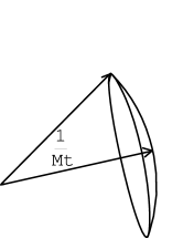
Figure 1: Sketch of the angle-smearing region (three-dimensional rendering)

The result is a regulated correlator

$$G_{M^{2}}(\vec{t},\vec{t}^{\prime})=\tfrac{1}{\int_{\hat{u}\in R_{M^{2}}(\vec{t})}d^{3}\hat{u}\int_{\hat{u}^{\prime}\in R_{M^{2}}(\vec{t}^{\prime})}d^{3}\hat{u}^{\prime}\,\,}\int_{\begin{subarray}{c}\hat{u}\in R_{M^{2}}(\vec{t})\\ \hat{u}^{\prime}\in R_{M^{2}}(\vec{t}^{\prime})\end{subarray}}d^{3}\hat{u}d^{3}\hat{u}^{\prime}\,G(t\hat{u},t^{\prime}\hat{u}^{\prime}).$$ (17)

We recall that our renormalized theory is determined by the translationally invariant function $I(\vec{t}-\vec{t}_{ave};\mu^{2})$ described in the previous section. Even though our regularization scheme breaks translational invariance, the renormalized theory nevertheless remains invariant.

As the radius $t$ increases the curvature of the angle-smearing region becomes negligible. In the limit $t\rightarrow\infty$ the region becomes a flat three-dimensional ball with radius $\tfrac{1}{M}$ lying in the plane perpendicular to the radial vector. In this limit our regularization is invariant under local transformations and the counterterms converge to constants independent of $\vec{t}$,

$$\lim_{t\rightarrow\infty}F_{\nabla\phi\nabla\phi}^{ij}(\vec{t}) =c_{\nabla\phi\nabla\phi}^{ij,(0)}(\tfrac{\mu^{2}}{M^{2}})$$ (18)

$$\lim_{t\rightarrow\infty}F_{\phi^{2}}(\vec{t}) =M^{2}c_{\phi^{2}}^{(0)}(\tfrac{\mu^{2}}{M^{2}})$$ (19)

$$\lim_{t\rightarrow\infty}F_{\phi^{4}}(\vec{t}) =c_{\phi^{4}}^{(0)}(\tfrac{\mu^{2}}{M^{2}}).$$ (20)

We have chosen our coefficients $c_{A}^{(0)}$ to be dimensionless. Although our regularization scheme is invariant under rotations about the origin, the radial vector has a special orientation which is normal to our three-dimensional ball. Our regularization scheme is therefore not isotropic. The result (as should be familiar from studies of anisotropic lattices) is that the coefficient of the kinetic term has two independent components

$$c_{\nabla\phi\nabla\phi}^{ij,(0)}(\tfrac{\mu^{2}}{M^{2}})=c_{\nabla\phi\nabla\phi}^{\hat{t}\hat{t},(0)}(\tfrac{\mu^{2}}{M^{2}})+\delta^{ij}c_{\nabla\phi\nabla\phi}^{(0)}(\tfrac{\mu^{2}}{M^{2}}).$$ (21)

Starting with the $t\rightarrow\infty$ result at lowest order, we now expand our coefficient functions in powers of $\frac{1}{Mt}$,

$$F_{\nabla\phi\nabla\phi}^{ij}(\vec{t}) =c_{\nabla\phi\nabla\phi}^{ij,(0)}(\tfrac{\mu^{2}}{M^{2}})+\tfrac{1}{Mt}c_{\nabla\phi\nabla\phi}^{ij,(1)}(\tfrac{\mu^{2}}{M^{2}})+\tfrac{1}{M^{2}t^{2}}c_{\nabla\phi\nabla\phi}^{ij,(2)}(\tfrac{\mu^{2}}{M^{2}})+\cdots$$ (22)

$$F_{\phi^{2}}(\vec{t}) =M^{2}c_{\phi^{2}}^{(0)}(\tfrac{\mu^{2}}{M^{2}})+\tfrac{M}{t}c_{\phi^{2}}^{(1)}(\tfrac{\mu^{2}}{M^{2}})+\tfrac{1}{t^{2}}c_{\phi^{2}}^{(2)}(\tfrac{\mu^{2}}{M^{2}})+\cdots$$ (23)

$$F_{\phi^{4}}(\vec{t}) =c_{\phi^{4}}^{(0)}(\tfrac{\mu^{2}}{M^{2}})+\tfrac{1}{Mt}c_{\phi^{4}}^{(1)}(\tfrac{\mu^{2}}{M^{2}})+\tfrac{1}{M^{2}t^{2}}c_{\phi^{4}}^{(2)}(\tfrac{\mu^{2}}{M^{2}})+\cdots.$$ (24)

For the moment let us assume $t\geq\Lambda^{-1}$ for

$$\Lambda=m_{0}^{z}M^{1-z},$$ (25)

for some fixed mass $m_{0}$ and constant $z$ such that $0<z<\frac{1}{2}$. In this region our dimensionless expansion parameter $\frac{1}{Mt}$ is bounded by $\tfrac{m_{0}^{z}}{M^{z}}$ and therefore diminishes uniformly as $M\rightarrow\infty$.

In general the $\tfrac{\mu^{2}}{M^{2}}$ dependence in the functions $c_{A}^{(k)}$ will contain analytic terms as $\mu^{2}\rightarrow 0$ as well as logarithmically divergent terms. There are, however, no inverse powers of $\tfrac{\mu^{2}}{M^{2}}$. These would indicate severe infrared divergences not present in the processes we are considering, as can be deduced from the long distance behavior of the integral in (9). With this we can neglect terms which vanish as $M\rightarrow\infty,$

$$F_{\phi^{2}}(\vec{t}) =M^{2}c_{\phi^{2}}^{(0)}(\tfrac{\mu^{2}}{M^{2}})+\tfrac{1}{t^{2}}c_{\phi^{2}}^{(2)}(\tfrac{\mu^{2}}{M^{2}})$$ (26)

$$F_{\nabla\phi\nabla\phi}^{ij}(\vec{t}) =c_{\nabla\phi\nabla\phi}^{ij,(0)}(\tfrac{\mu^{2}}{M^{2}})$$ (27)

$$F_{\phi^{4}}(\vec{t}) =c_{\phi^{4}}^{(0)}(\tfrac{\mu^{2}}{M^{2}}).$$ (28)

Since our regularization scheme is invariant under $M\rightarrow-M$, we have also omitted the term proportional  to $c_{\phi^{2}}^{(1)}$ which is odd in $M$.

We now consider what occurs in the small region near the origin, $t\leq\Lambda^{-1}$. For the theory we are considering (and in fact for any renormalizable theory) the highest ultraviolet divergence possible is quadratic. In the limit $M\rightarrow\infty$ we deduce that each $F_{A}$ scales no greater than $O(M^{2}).$ On the other hand the volume of the region $t\leq\Lambda^{-1}$ diminishes as $O(M^{4z-4}).$ Thus the total contribution from the region $t\leq\Lambda^{-1}$ scales as $O(M^{4z-2})$ and can be entirely neglected.

To summarize our results, the counterterm Lagrange density has the form

$$c_{\nabla\phi\nabla\phi}^{(0)}(\vec{\nabla}\phi(\vec{t}))^{2}+c_{\nabla\phi\nabla\phi}^{\hat{t}\hat{t},(0)}(\hat{t}\cdot\vec{\nabla}\phi(\vec{t}))^{2}+(M^{2}c_{\phi^{2}}^{(0)}+\tfrac{1}{t^{2}}c_{\phi^{2}}^{(2)})\phi^{2}(\vec{t})+c_{\phi^{4}}^{(0)}\phi^{4}(\vec{t}).$$ (29)

4 Spherical fields

We now examine the results of the previous section in the context of spherical field theory. We start with the spherical partial wave expansion,

$$\phi={\textstyle\sum_{l=0,1,\cdots}}{\textstyle\sum_{n=0,\cdots l}}{\textstyle\sum_{m=-n,\cdots n}}\phi_{l,n,m}(t)Y_{l,n,m}(\theta,\psi,\varphi),$$ (30)

where $Y_{l,m,n}$ are four-dimensional spherical harmonics satisfying

$${\textstyle\int}d^{3}\Omega\,Y_{l^{\prime},n^{\prime},m^{\prime}}^{\ast}(\theta,\psi,\varphi)Y_{l,n,m}(\theta,\psi,\varphi)=\delta_{l^{\prime},l}\delta_{n^{\prime},n}\delta_{m^{\prime},m},$$ (31)

$$Y_{l,n,m}^{\ast}(\theta,\psi,\varphi)=(-1)^{m}Y_{l,n,-m}(\theta,\psi,\varphi).$$ (32)

The explicit form of $Y_{l,m,n}$ can be found in [14]. The integral of the free massless Lagrange density in terms of spherical fields is

$${\textstyle\int}d^{4}\vec{t}\,\mathcal{L}={\textstyle\int_{0}^{\infty}}dt\,\left\{\sum_{l,m,n}\left[(-1)^{m}\phi_{l,n,-m}\left[\tfrac{\partial}{\partial t}\tfrac{t^{3}}{2}\tfrac{\partial}{\partial t}-\tfrac{t}{2}l(l+2)\right]\phi_{l,n,m}\right]\right\}.$$ (33)

It can be shown that the process of angle smearing the field $\phi(\vec{t})$ is equivalent to multiplying $\phi_{l,n,m}(t)$ by an extra factor $s_{l}^{M}(t)$ where

$$s_{l}^{M}(t)=\tfrac{2Mt\left[(l+2)\sin(\frac{l}{Mt})-l\sin(\frac{l+2}{Mt})\right]}{l(l+1)(l+2)\left[2-Mt\sin(\frac{2}{Mt})\right]}.$$ (34)

For large $l$, $s_{l}^{M}(t)$ diminishes as $l^{-2}$, and so the correlator receives an extra suppression of $l^{-4}$. We will later use this result to estimate the contribution of high spin partial waves. The regularization of our correlator can be implemented in our Lagrange density by dividing factors of $s_{l}^{M}(t),$

$$\phi_{l,n,-m}\left[\tfrac{\partial}{\partial t}\tfrac{t^{3}}{2}\tfrac{\partial}{\partial t}-\tfrac{t}{2}l(l+2)\right]\phi_{l,n,m}$$ (35)

$$\rightarrow\left[(s_{l}^{M}(t))^{-1}\phi_{l,n,-m}\right]\left[\tfrac{\partial}{\partial t}\tfrac{t^{3}}{2}\tfrac{\partial}{\partial t}-\tfrac{t}{2}l(l+2)\right]\left[(s_{l}^{M}(t))^{-1}\phi_{l,n,m}\right].$$

We now include the interaction and counterterms. We first define

$$\left[\genfrac{}{}{0.0pt}{1}{l_{1},n_{1},m_{1};l_{2},n_{2},m_{2}}{l_{3},n_{3},m_{3};l_{4},n_{4},m_{4}}\right]$$ (36)

$$={\textstyle\int}d^{3}\Omega\,Y_{l_{1},n_{1},m_{1}}(\theta,\psi,\varphi)Y_{l_{2},n_{2},m_{2}}(\theta,\psi,\varphi)Y_{l_{3},n_{3},m_{3}}(\theta,\psi,\varphi)Y_{l_{4},n_{4},m_{4}}(\theta,\psi,\varphi).$$

We can write the full functional integral as

$$\int\mathcal{D}\phi\exp\left[{\textstyle\int}d^{4}\vec{t}\,\mathcal{L}\right]\propto\int\left({\textstyle\prod_{l,n,m}}\mathcal{D}\phi_{l,n,m}^{\prime}\right)\exp\left[{\textstyle\int_{0}^{\infty}}dt\,(L_{1}+L_{2}+L_{3})\right],$$ (37)

where

$$L_{1}=\sum_{l,m,n}\left[(-1)^{m}\left[(s_{l}^{M}(t))^{-1}\phi_{l,n,-m}^{\prime}\right]\left[\tfrac{\partial}{\partial t}\tfrac{t^{3}}{2}\tfrac{\partial}{\partial t}-\tfrac{t}{2}l(l+2)\right]\left[(s_{l}^{M}(t))^{-1}\phi_{l,n,m}^{\prime}\right]\right],$$ (38)

$$L_{2}=\sum_{l,m,n}\left[(-1)^{m}\phi_{l,n,-m}^{\prime}\left[\begin{array}[c]{c}\left[-c_{\nabla\phi\nabla\phi}^{(0)}-c_{\nabla\phi\nabla\phi}^{\hat{t}\hat{t},(0)}\right]\tfrac{\partial}{\partial t}\tfrac{t^{3}}{2}\tfrac{\partial}{\partial t}\\ +c_{\nabla\phi\nabla\phi}^{(0)}\tfrac{t}{2}l(l+2)+t^{3}(M^{2}c_{\phi^{2}}^{(0)}+\tfrac{1}{t^{2}}c_{\phi^{2}}^{(2)})\end{array}\right]\phi_{l,n,m}^{\prime}\right],$$ (39)

$$L_{3}=-t^{3}(\tfrac{\lambda}{4!}-c_{\phi^{4}}^{(0)})\sum_{l_{i},m_{i},n_{i}}\left[\genfrac{}{}{0.0pt}{1}{l_{1},m_{1},n_{1};l_{2},m_{2},n_{2}}{l_{3},m_{3},n_{3};l_{4},m_{4},n_{4}}\right]\phi_{l_{1},m_{1},n_{1}}^{\prime}\phi_{l_{2},m_{2},n_{2}}^{\prime}\phi_{l_{3},m_{3},n_{3}}^{\prime}\phi_{l_{4},m_{4},n_{4}}^{\prime}.$$ (40)

We have used primes in preparation for redefining the fields,

$$(s_{l}^{M}(t))^{-1}\phi_{l,n,m}^{\prime}=\phi_{l,n,m}.$$ (41)

The Jacobian of this transformation is a constant (although infinite) and can be absorbed into the normalization of the functional integral. Now the Lagrangian $L_{1}$ has the usual free-field form in terms of $\phi_{l,n,m}$ while $L_{2}$ and $L_{3}$ are now functions of $s_{l}^{M}(t)\phi_{l,n,m}$.

With $M$ serving as our ultraviolet regulator, the contribution of high-spin partial waves decouples for sufficiently large spin $l$. We can estimate the order of magnitude of this contribution in the following manner. We first identify $t^{-1}l$ (where $t$ is the characteristic radius we are considering) as an estimate of the magnitude of the tangential momentum, $p_{T}$. For $p_{T}\gg M\gg t^{-1}$ our correlator scales as $\tfrac{M^{4}}{p_{T}^{6}}.$ By dimensional analysis, a diagram with $N_{L}$ loops and $N_{I}$ internal lines will receive a contribution from partial waves with spin $\geq l$ of order

$$\left(\tfrac{M^{4}}{p_{T}^{6}}\right)^{N_{I}}\left(p_{T}\right)^{4N_{L}}=\left(\tfrac{M^{4}}{(t^{-1}l)^{6}}\right)^{N_{I}}\left(t^{-1}l\right)^{4N_{L}}.$$ (42)

5 One-loop examples

We will devote the remainder of our discussion to computing one-loop spherical Feynman diagrams as a check of our results. Our calculations are done both numerically and analytically. The diagrams we will consider are shown in Figures 2 and 3.

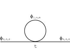
Figure 2: One-loop two-point correlator for $\phi_{0,0,0}$

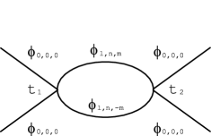
Figure 3: One-loop four-point correlator for $\phi_{0,0,0}$

We start with the two-point function in Figure 2. The amplitude can be written as $t^{3}B(t)$ where

$$B(t)\propto{\textstyle\sum_{l,n,m}}\tfrac{1}{t^{2}(l+1)}(s_{l}^{M}(t))^{2}.$$ (43)

Constants of proportionality are not important here and so we will define $B(t)$ to be equal to the right side of (43). Our results tell us that if we choose our mass counterterms appropriately, the combination

$$B(t)+M^{2}c_{\phi^{2}}^{(0)}+\tfrac{1}{t^{2}}c_{\phi^{2}}^{(2)}$$ (44)

should be independent of $t$, or more succinctly,

$$B(t)+\tfrac{1}{t^{2}}c_{\phi^{2}}^{(2)}$$ (45)

is independent of $t$. Let us first check this analytically. In the absence of a high-spin cutoff, we can explicitly calculate the sum in (43):

$$B(t)=\tfrac{1}{t^{2}}+b(t)$$ (46)

where

$$b(t)=\tfrac{4M^{2}\sin^{4}(\frac{1}{Mt})}{(2-Mt\sin(\frac{2}{Mt}))^{2}}.$$ (47)

In the limit $M\rightarrow\infty,$

$$B(t)\rightarrow\tfrac{1}{t^{2}}+\tfrac{9}{4}M^{2}.$$ (48)

We conclude that $c_{\phi^{2}}^{(2)}=-1$ and $B(t)+\tfrac{1}{t^{2}}c_{\phi^{2}}^{(2)}$ is in fact translationally invariant.

In Figure 4

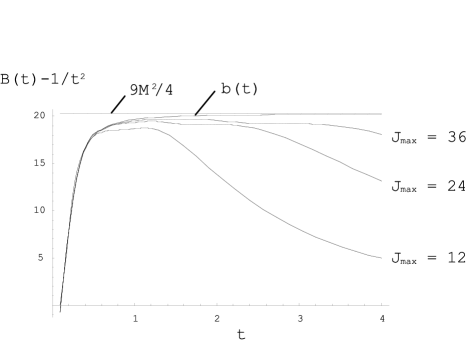
Figure 4: Plot of $B(t)-\tfrac{1}{t^{2}}$

we have plotted $B(t)-\tfrac{1}{t^{2}}$, computed numerically for various values of the high-spin cutoff $J_{\max}$. We have also plotted the limiting values $b(t)$ and $\tfrac{9}{4}M^{2}$. In our plot $t$ is measured in units of $m^{-1}$ and $B(t)-\tfrac{1}{t^{2}}$ is in units of $m^{2}$, where $m$ is an arbitrary mass scale such that $M=3m$. As expected, the errors are of size $\frac{M^{4}t^{2}}{J_{\max}^{2}}$. There is clearly a deviation from $\tfrac{9}{4}M^{2}$ for $t\lesssim M^{-1}$ but the integral of the deviation is negligible as $M\rightarrow\infty$.

We now turn to the four-point function in Figure 3. The amplitude can be written as $t_{1}^{3}t_{2}^{3}C(t_{1},t_{2})$ where

$$C(t_{1},t_{2})\propto{\textstyle\sum_{l,n,m}}\tfrac{(s_{l}^{M}(t_{1}))^{2}(s_{l}^{M}(t_{2}))^{2}}{(l+1)^{2}}\left[\tfrac{t_{1}^{l}}{t_{2}^{l+2}}\theta(t_{2}-t_{1})+\tfrac{t_{2}^{l}}{t_{1}^{l+2}}\theta(t_{1}-t_{2})\right]^{2}.$$ (49)

Again constants of proportionally are not important and so we will define $C(t_{1},t_{2})$ to be equal to the right side of (49). We can write $C(t_{1},t_{2})$ in terms of the regulated correlator $G_{M^{2}}(\vec{t}_{1},\vec{t}_{2}),$

$$C(t_{1},t_{2})\propto\int d^{3}\hat{t}_{1}d^{3}\hat{t}_{2}\left[G_{M^{2}}(\vec{t}_{1},\vec{t}_{2})\right]^{2}\propto\int d^{3}\hat{t}_{1}\left[G_{M^{2}}(\vec{t}_{1},\vec{t}_{2})\right]^{2}.$$ (50)

Since the coupling constant counterterm

$$c_{\phi^{4}}^{(0)}\delta^{4}(\vec{t}_{1}-\vec{t}_{2})$$ (51)

is translationally invariant, the amplitude by itself should be translationally invariant. Let us define

$$\int d^{4}\vec{t}_{2}e^{-i\vec{p}\cdot(\vec{t}_{1}-\vec{t}_{2})}\left[G_{M^{2}}(\vec{t}_{1},\vec{t}_{2})\right]^{2}=f(\vec{p}^{2}),$$ (52)

so that

$$\int d^{4}\vec{t}_{2}e^{i\vec{p}\cdot\vec{t}_{2}}\left[G_{M^{2}}(\vec{t}_{1},\vec{t}_{2})\right]^{2}=e^{i\vec{p}\cdot\vec{t}_{1}}f(\vec{p}^{2}).$$ (53)

Integrating over $\hat{t}_{1}$, we find

$$\int dt_{2}\,t_{2}^{2}J_{1}(pt_{2})C(t_{1},t_{2})\propto\tfrac{1}{t_{1}}J_{1}(pt_{1})f(\vec{p}^{2}).$$ (54)

Let us define

$$C(t)={\textstyle\int}dt_{2}\,t_{2}^{2}J_{1}(pt_{2})C(t,t_{2}).$$ (55)

We now check that in fact

$$C(t)\propto\tfrac{1}{t_{1}}J_{1}(pt_{1})\text{.}$$ (56)

In the absence of a high-spin cutoff, we find that $C(t)$ is given by

$$C(t)=\tfrac{1}{t_{1}}J_{1}(pt_{1})\left[\tfrac{1}{2}\log\tfrac{M^{2}}{p^{2}}+c\right]+\cdots,$$ (57)

where the ellipsis represents terms which vanish as $M\rightarrow\infty$ and

$$c=324\left[\int_{0}^{1/2}dk\left(\tfrac{(\sin k-k\cos k)^{4}}{4k^{13}}-\tfrac{1}{324k}\right)+\int_{1/2}^{\infty}dk\tfrac{(\sin k-k\cos k)^{4}}{4k^{13}}\right].$$ (58)

In Figure 5

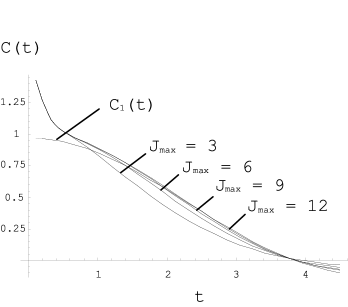
Figure 5: Plot of $C(t)$

we plot $C(t)$ for different values of the high-spin cutoff $J_{\max}$ as well as the large-$M$ limit value

$$C_{1}(t)=\tfrac{1}{t_{1}}J_{1}(pt_{1})\left[\tfrac{1}{2}\log\tfrac{M^{2}}{p^{2}}+c\right].$$ (59)

In our plot $t$ is measured in units of $p^{-1}$ and $M=3p$. From (42) the expected error is of size $\frac{M^{8}t^{8}}{J_{\max}^{8}}.$ We see that the data is consistent with the results expected. Again the deviation for $t\lesssim M^{-1}$ integrates to a negligible contribution as $M\rightarrow\infty$.

6 Summary

We have examined several important features of non-perturbative renormalization in the spherical field formalism and answered the three questions posed in the introduction. Ultraviolet divergences can be cancelled by a finite number of local counterterms in a manner such that the renormalized theory is translationally invariant. Using angle-smearing regularization we find that the counterterms for $\phi^{4}$ theory in four dimensions can be parameterized by five unknown constants as shown in (29). Aside from our remarks about Ward identity constraints in gauge theories, the extension to other field theories is straightforward. We hope that these results will be useful for future studies of general renormalizable theories by spherical field techniques.

Chapter 2 The massless Thirring model in spherical field theory

1 Introduction

The massless Thirring model [58] is an exactly soluble system of a single self-interacting massless fermion in two dimensions.  There are a number of solutions in the literature based on properties of the Euler-Lagrange equations and fermion currents or bosonization techniques [30, 55, 20, 16, 31, 12, 57, 15, 45, 59, 44].  Given its simplicity and solubility, the model has become a popular testing ground for new ideas and methods in field theory.

From a computational point of view, however, the massless Thirring model still presents a significant challenge. In the lattice field formalism, the difficulties are due to the appearance of fermion doubler states and singular inversion problems associated with integrating out massless fermions.  In this work we use the model to illustrate new non-perturbative methods in the spherical field formalism [35, 36, 5, 38].  The techniques we present are quite general and can also be applied to other modal expansion methods such as periodic field theory [43].

As noted in [36], we will not need to worry about fermion doubling.  This is true for any modal field theory and follows from the fact that space is not discretized but retained as a continuous variable.  Since our model is not super-renormalizable we will use a procedure called angle-smearing, a regularization method designed for spherical field theory [38].  With angle-smearing regularization and a small set of local counterterms, we are able to remove all ultraviolet divergences in a manner such that the renormalized theory is finite and translationally invariant.  Comparison of our results with the known Thirring model solution will serve as a consistency check for our regularization and renormalization procedures.

The organization of this paper is as follows.  We begin with a short summary of the massless Thirring model, following the solution of Hagen [20]. Using angle-smearing regularization we obtain the spherical field Hamiltonian and construct a matrix representation of the Hamiltonian. We reduce the space of states using a two-parameter auxiliary cutoff procedure.  In this reduced space we compute the time evolution of quantum states using a fourth-order Runge-Kutta-Fehlberg algorithm.  We calculate the two point correlator for several values of the coupling and find agreement with the known analytic solution.

2 The model

We start with a list of our notational conventions.  Our analysis will be in two-dimensional Euclidean space, and we use both cartesian and polar coordinates,

$$\vec{t}=(t\cos\theta,t\sin\theta)=(x,y).$$ (1)

The components of the spinors $\psi$ and $\bar{\psi}$ are written as

$$\psi=\left[\begin{array}[c]{c}\psi^{\uparrow}\\ \psi^{\downarrow}\end{array}\right]\qquad\bar{\psi}=\left[\begin{array}[c]{cc}\bar{\psi}^{\uparrow}&\bar{\psi}^{\downarrow}\end{array}\right].$$ (2)

Our representation for the Dirac matrices is

$$\vec{\gamma}=i\vec{\sigma},$$ (3)

and so $\vec{\gamma}$ satisfies

$$\left\{\gamma^{i},\gamma^{j}\right\}=-2\delta^{ij},\qquad i,j=1,2.$$ (4)

The massless Thirring model is formally defined by the Lagrange density

$$\mathcal{L}=i\bar{\psi}\vec{\gamma}\cdot\vec{\nabla}\psi-\tfrac{\lambda}{2}\,\vec{j}\cdot\vec{j},$$ (5)

where $\vec{j}$ is the fermion vector current.  Johnson [30] emphasized the importance of defining the regularized current precisely, and this was further clarified by the work of Sommerfield [55] and Hagen [20]. We will use a regularization technique, introduced in [38], called angle-smearing. We define the regularized current as

$$\vec{j}=\tfrac{1}{2}\left(\bar{\psi}_{s}\vec{\gamma}\psi_{s}-Tr[\vec{\gamma}\psi_{s}\bar{\psi}_{s}]\right),$$ (6)

where

$$\psi_{s}(t,\theta)=\tfrac{Mt}{2}\int_{-\frac{1}{Mt}}^{\frac{1}{Mt}}d\varepsilon\psi(t,\theta+\varepsilon).$$ (7)

We identify the radial variable $t$ as our time parameter, and our definition of the current is local with respect to $t$.

Hagen [20] described the solution of the Thirring model in the Hamiltonian formalism with currents defined as products of the canonical operators at equal times. Though our equal-time surface is curved, the curvature of the integration segment in (7) scales as $\frac{1}{M}$ while the ultraviolet divergences in this model are only logarithmic in $M$. In the $M\rightarrow\infty$ limit we therefore recover the standard results. As discussed in [20], there exists a one parameter class of solutions to the Thirring model depending on the preferred definition of the regularized vector and axial vector currents. We will use the conventions used in [30] and [55], which in Hagen’s notation corresponds with the parameter values $\xi=\eta=\frac{1}{2}$.  With this choice the Hamiltonian density takes the form

$$\mathcal{H}=\mathcal{H}_{free}+\tfrac{\pi c}{1-c}(\hat{t}\cdot\vec{j})^{2}+\tfrac{\pi c}{1+c}(\hat{\theta}\cdot\vec{j})^{2},$$ (8)

where

$$c=\tfrac{\lambda}{2\pi}\text{.}$$ (9)

The only counterterms needed in this model are wavefunction renormalization counterterms, a result of our careful definition for the regularized interaction in (8). As in [20] we calculate correlation functions using an unrenormalized Hamiltonian.  The divergent wavefunction normalizations will appear simply as overall factors in the correlators.

3 Spherical field Hamiltonian

In this section we derive the form of the spherical field Hamiltonian. We first expand the fermion current in terms of components of the spinors,

$$\hat{t}\cdot\bar{\psi}_{s}\vec{\gamma}\psi_{s}=i\bar{\psi}_{s}\left[\begin{array}[c]{cc}0&e^{-i\theta}\\ e^{i\theta}&0\end{array}\right]\psi_{s}=ie^{-i\theta}\bar{\psi}_{s}^{\uparrow}\psi_{s}^{\downarrow}+ie^{i\theta}\bar{\psi}_{s}^{\downarrow}\psi_{s}^{\uparrow}$$ (10)

$$\hat{\theta}\cdot\bar{\psi}_{s}\vec{\gamma}\psi_{s}=\bar{\psi}_{s}\left[\begin{array}[c]{cc}0&e^{-i\theta}\\ -e^{i\theta}&0\end{array}\right]\psi_{s}=e^{-i\theta}\bar{\psi}_{s}^{\uparrow}\psi_{s}^{\downarrow}-e^{i\theta}\bar{\psi}_{s}^{\downarrow}\psi_{s}^{\uparrow}.$$ (11)

The anti-commutators of the regulated fields are

$$\left\{\bar{\psi}_{s}^{\uparrow},\psi_{s}^{\downarrow}\right\}=\tfrac{1}{t}\left(\tfrac{Mt}{2}\right)^{2}{\textstyle\int_{-\frac{1}{Mt}}^{\frac{1}{Mt}}}e^{i(\theta+\varepsilon)}d\varepsilon=A(t)e^{i\theta}$$ (12)

$$\left\{\bar{\psi}_{s}^{\downarrow},\psi_{s}^{\uparrow}\right\}=\tfrac{1}{t}\left(\tfrac{Mt}{2}\right)^{2}{\textstyle\int_{-\frac{1}{Mt}}^{\frac{1}{Mt}}}e^{-i(\theta+\varepsilon)}d\varepsilon=A(t)e^{-i\theta},$$ (13)

where

$$A(t)=\tfrac{M^{2}t}{2}\sin(\tfrac{1}{Mt}).$$ (14)

From the anti-commutation relations, the $\hat{t}$ component of the current is

$$\hat{t}\cdot\vec{j} =\tfrac{1}{2}\left[ie^{-i\theta}(\bar{\psi}_{s}^{\uparrow}\psi_{s}^{\downarrow}-\psi_{s}^{\downarrow}\bar{\psi}_{s}^{\uparrow})+ie^{i\theta}(\bar{\psi}_{s}^{\downarrow}\psi_{s}^{\uparrow}-\psi_{s}^{\uparrow}\bar{\psi}_{s}^{\downarrow})\right]$$ (15)

$$=ie^{-i\theta}\bar{\psi}_{s}^{\uparrow}\psi_{s}^{\downarrow}+ie^{i\theta}\bar{\psi}_{s}^{\downarrow}\psi_{s}^{\uparrow}-iA(t),$$

and so

$$(\hat{t}\cdot\vec{j})^{2}=A(t)\left[e^{-i\theta}\bar{\psi}_{s}^{\uparrow}\psi_{s}^{\downarrow}+e^{i\theta}\bar{\psi}_{s}^{\downarrow}\psi_{s}^{\uparrow}\right]-2\bar{\psi}_{s}^{\uparrow}\psi_{s}^{\downarrow}\bar{\psi}_{s}^{\downarrow}\psi_{s}^{\uparrow}-A^{2}(t).$$ (16)

Similarly we find

$$(\hat{\theta}\cdot\vec{j})^{2}=A(t)\left[e^{-i\theta}\bar{\psi}_{s}^{\uparrow}\psi_{s}^{\downarrow}+e^{i\theta}\bar{\psi}_{s}^{\downarrow}\psi_{s}^{\uparrow}\right]-2\bar{\psi}_{s}^{\uparrow}\psi_{s}^{\downarrow}\bar{\psi}_{s}^{\downarrow}\psi_{s}^{\uparrow}.$$ (17)

The Hamiltonian can now be written as

$$H=H_{free}+\int d\theta\,t\left\{\tfrac{2\pi c}{1-c^{2}}\left[A(t)\left[e^{-i\theta}\bar{\psi}_{s}^{\uparrow}\psi_{s}^{\downarrow}+e^{i\theta}\bar{\psi}_{s}^{\downarrow}\psi_{s}^{\uparrow}\right]-2\bar{\psi}_{s}^{\uparrow}\psi_{s}^{\downarrow}\bar{\psi}_{s}^{\downarrow}\psi_{s}^{\uparrow}\right]\right\}.$$ (18)

We have omitted the constant term proportional to $A^{2}(t)$.

Let us define the partial wave modes

$$\psi_{n}(t) =\tfrac{1}{\sqrt{2\pi}}\int d\theta\,e^{-in\theta}\psi(\vec{t}),\qquad\psi_{s,n}(t)=\tfrac{1}{\sqrt{2\pi}}\int d\theta\,e^{-in\theta}\psi_{s}(\vec{t}),$$ (19)

$$\bar{\psi}_{n}(t) =\tfrac{1}{\sqrt{2\pi}}\int d\theta\,e^{-in\theta}\bar{\psi}(\vec{t}),\qquad\bar{\psi}_{s,n}(t)=\tfrac{1}{\sqrt{2\pi}}\int d\theta\,e^{-in\theta}\bar{\psi}_{s}(\vec{t}).$$ (20)

It is straightforward to show that for $n\neq 0,$

$$\psi_{s,n}(t)=\tfrac{\sin(\frac{n}{Mt})}{\left(\frac{n}{Mt}\right)}\psi_{n}(t)\qquad\bar{\psi}_{s,n}(t)=\tfrac{\sin(\frac{n}{Mt})}{\left(\frac{n}{Mt}\right)}\bar{\psi}_{n}(t).$$ (21)

We can extend this result to the case $n=0$ using the convenient shorthand

$$\tfrac{\sin(\frac{0}{Mt})}{\left(\frac{0}{Mt}\right)}\equiv 1.$$ (22)

At this point it is convenient to rescale $\bar{\psi}$,

$$\bar{\psi}_{n}^{i\prime}=t\bar{\psi}_{n}^{i}.$$ (23)

In terms of the partial waves,

$$H= \tfrac{1}{t}\sum_{n}\left[\left(n+1+\tfrac{b\pi tA(t)\sin(\frac{n}{Mt})\sin(\frac{n+1}{Mt})}{\left(\frac{n}{Mt}\right)\left(\frac{n+1}{Mt}\right)}\right)\bar{\psi}_{-n}^{\uparrow\prime}\psi_{n+1}^{\downarrow}\right]$$ (24)

$$-\tfrac{1}{t}\sum_{n}\left[\left(n-\tfrac{b\pi tA(t)\sin(\frac{n}{Mt})\sin(\frac{n+1}{Mt})}{\left(\frac{n}{Mt}\right)\left(\frac{n+1}{Mt}\right)}\right)\bar{\psi}_{-n-1}^{\downarrow\prime}\psi_{n}^{\uparrow}\right]$$

$$-\sum_{-n_{1}+n_{2}-n_{3}+n_{4}=0}\left[\tfrac{b}{t}\bar{\psi}_{-n_{1}}^{\uparrow\prime}\psi_{n_{2}+1}^{\downarrow}\bar{\psi}_{-n_{3}-1}^{\downarrow\prime}\psi_{n_{4}}^{\uparrow}\tfrac{\sin(\frac{n_{1}}{Mt})\sin(\frac{n_{2}+1}{Mt})\sin(\frac{n_{3}+1}{Mt})\sin(\frac{n_{4}}{Mt})}{\left(\frac{n_{1}}{Mt}\right)\left(\frac{n_{2}+1}{Mt}\right)\left(\frac{n_{3}+1}{Mt}\right)\left(\frac{n_{4}}{Mt}\right)}\right],$$

where

$$b=\tfrac{2c}{1-c^{2}}.$$ (25)

Since $b$ is the parameter appearing in the Hamiltonian, it is somewhat more convenient to express $c$ in terms of $b,$

$$c=\tfrac{\sqrt{1+b^{2}}-1}{b}.$$ (26)

Let us define the ladder operators

$$a_{-n}^{\uparrow},a_{-n}^{\uparrow\dagger} \equiv\psi_{n}^{\uparrow},\bar{\psi}_{-n-1}^{\downarrow\prime}$$ (27)

$$a_{n+1}^{\downarrow},a_{n+1}^{\downarrow\dagger} \equiv\psi_{n+1}^{\downarrow},\bar{\psi}_{-n}^{\uparrow\prime}.$$ (28)

These operators satisfy the anti-commutation relations

$$\left\{a_{n_{1}}^{\downarrow},a_{n_{2}}^{\downarrow\dagger}\right\}=\left\{a_{n_{1}}^{\uparrow},a_{n_{2}}^{\uparrow\dagger}\right\}=\delta_{n_{1}n_{2}},$$ (29)

with all other anti-commutators equal to zero. We can now recast the Hamiltonian as

$$H =\tfrac{1}{t}\sum_{n}\left[n+\tfrac{b\pi tA(t)\sin(\frac{n}{Mt})\sin(\frac{n-1}{Mt})}{\left(\frac{n}{Mt}\right)\left(\frac{n-1}{Mt}\right)}\right]\left(a_{n}^{\downarrow\dagger}a_{n}^{\downarrow}+a_{n}^{\uparrow\dagger}a_{n}^{\uparrow}\right)$$ (30)

$$-\sum_{-n_{1}+n_{2}+n_{3}-n_{4}=0}\left[\tfrac{b}{t}a_{n_{1}}^{\downarrow\dagger}a_{n_{2}}^{\downarrow}a_{n_{3}}^{\uparrow\dagger}a_{n_{4}}^{\uparrow}\tfrac{\sin(\frac{n_{1}-1}{Mt})\sin(\frac{n_{2}}{Mt})\sin(\frac{n_{3}-1}{Mt})\sin(\frac{n_{4}}{Mt})}{\left(\frac{n_{1}-1}{Mt}\right)\left(\frac{n_{2}}{Mt}\right)\left(\frac{n_{3}-1}{Mt}\right)\left(\frac{n_{4}}{Mt}\right)}\right].$$

We will implement a high spin cutoff by removing terms in the interaction containing operators $a_{n}^{\downarrow}$, $a_{n}^{\uparrow},$ $a_{n}^{\downarrow\dagger}$, or $a_{n}^{\uparrow\dagger}$ for $\left|n\right|>J_{\max}$. This has the effect of removing high spin modes, which correspond with large tangential momentum states.  We should emphasize, however, that $J_{\max}$ is an auxiliary cutoff. It does not play a role in the regularization scheme since the interactions have already been rendered finite using angle-smearing.  The contribution of these high spin modes is negligible so long as

$$\tfrac{J_{\max}}{t}\gg M,$$ (31)

where $t$ is the characteristic radius of the process being measured.  Returning back to (12) and (13) and removing the contribution of these partial waves, we find that $A(t)$ is replaced by

$$A_{J_{\max}}(t)=\tfrac{1}{2\pi t}\sum_{n=-J_{\max}}^{J_{\max}}\tfrac{\sin(\frac{n}{Mt})}{\left(\frac{n}{Mt}\right)}\tfrac{\sin(\frac{n-1}{Mt})}{\left(\frac{n-1}{Mt}\right)}.$$ (32)

Let $\left|0\right\rangle_{free}$ be the ground state of the free massless fermion Hamiltonian. For $n>0,$ we find

$$a_{n}^{\downarrow}\left|0\right\rangle_{free}=a_{n}^{\uparrow}\left|0\right\rangle_{free}=0,$$ (33)

and for $n\leq 0,$

$$a_{n}^{\downarrow\dagger}\left|0\right\rangle_{free}=a_{n}^{\uparrow\dagger}\left|0\right\rangle_{free}=0.$$ (34)

It is convenient to define the normal-ordered products

$$\text{{}}\text{:{}}a_{n}^{\downarrow\dagger}a_{n}^{\downarrow}\text{:}=\left\{\begin{array}[c]{c}a_{n}^{\downarrow\dagger}a_{n}^{\downarrow}\text{ for }n>0\\ -a_{n}^{\downarrow}a_{n}^{\downarrow\dagger}\text{ for }n\leq 0\end{array}\right.\qquad\text{:{}}a_{n}^{\uparrow\dagger}a_{n}^{\uparrow}\text{:}=\left\{\begin{array}[c]{c}a_{n}^{\uparrow\dagger}a_{n}^{\uparrow}\text{ for }n>0\\ -a_{n}^{\uparrow}a_{n}^{\uparrow\dagger}\text{ for }n\leq 0.\end{array}\right.$$ (35)

The ordering for other operators is immaterial since the anti-commutators are zero. We can now rewrite $H$ in terms of normal-ordered products,

$$H =\left(\tfrac{n}{t}+O(J_{\max}^{-2})\right)\left(a_{n}^{\downarrow\dagger}a_{n}^{\downarrow}+a_{n}^{\uparrow\dagger}a_{n}^{\uparrow}\right)$$ (36)

$$-\sum_{-n_{1}+n_{2}+n_{3}-n_{4}=0}\left[\tfrac{b}{t}\text{:}a_{n_{1}}^{\downarrow\dagger}a_{n_{2}}^{\downarrow}a_{n_{3}}^{\uparrow\dagger}a_{n_{4}}^{\uparrow}\text{:}\tfrac{\sin(\frac{n_{1}-1}{Mt})\sin(\frac{n_{2}}{Mt})\sin(\frac{n_{3}-1}{Mt})\sin(\frac{n_{4}}{Mt})}{\left(\frac{n_{1}-1}{Mt}\right)\left(\frac{n_{2}}{Mt}\right)\left(\frac{n_{3}-1}{Mt}\right)\left(\frac{n_{4}}{Mt}\right)}\right].$$

There is an $O(J_{\max}^{-2})$ term due to a small asymmetry in our cutoff procedure with respect to the two boundaries $-J_{\max}$ and $J_{\max}$. We will neglect this term in the limit $J_{\max}\rightarrow\infty$.

4 Two-point correlator

We wish to study the properties of the two-point correlator. The massless Thirring model is invariant under the discrete transformation

$$\psi^{\downarrow}(\vec{t}),\bar{\psi}^{\uparrow}(\vec{t})\rightarrow-\psi^{\downarrow}(\vec{t}),-\bar{\psi}^{\uparrow}(\vec{t}),$$ (37)

as well as the transformation

$$\psi^{\uparrow}(t,\theta),\bar{\psi}^{\uparrow}(t,\theta)\leftrightarrow\psi^{\downarrow}(t,-\theta),\bar{\psi}^{\downarrow}(t,-\theta).$$ (38)

From these we deduce

$$\left\langle 0\right|T\left[\bar{\psi}^{\uparrow}(\vec{t})\psi^{\uparrow}(0)\right]\left|0\right\rangle=\left\langle 0\right|T\left[\bar{\psi}^{\downarrow}(\vec{t})\psi^{\downarrow}(0)\right]\left|0\right\rangle=0$$ (39)

and

$$\left\langle 0\right|T\left[\bar{\psi}^{\uparrow}(t,\theta)\psi^{\downarrow}(0)\right]\left|0\right\rangle=\left\langle 0\right|T\left[\bar{\psi}^{\downarrow}(t,-\theta)\psi^{\uparrow}(0)\right]\left|0\right\rangle.$$ (40)

It therefore suffices to consider just the correlator on the left side of (40).

In the limit $M\rightarrow\infty$ the form of the correlator is given by

$$\left\langle 0\right|T\left[\bar{\psi}^{\uparrow}(t,\theta)\psi^{\downarrow}(0)\right]\left|0\right\rangle=\tfrac{e^{i\theta}}{2\pi}(k(c)M)^{\frac{-2c^{2}}{1-c^{2}}}t^{\frac{-1-c^{2}}{1-c^{2}}},$$ (41)

where $k(c)$ is a dimensionless parameter.  Standard analytic methods do not yield a simple closed form expression for $k(c).$  We will therefore extract $k(c)$ from the computed value of the correlator at a specific renormalization point $t=t_{0}$.

We define

$$f(t)=\left\langle 0\right|T\left[\bar{\psi}_{1}^{\uparrow}(t)\psi_{0}^{\downarrow}(0)\right]\left|0\right\rangle.$$ (42)

Since

$$\left\langle 0\right|T\left[\bar{\psi}^{\uparrow}(t,\theta)\psi^{\downarrow}(0)\right]\left|0\right\rangle=\tfrac{e^{i\theta}}{2\pi}\left\langle 0\right|T\left[\bar{\psi}_{1}^{\uparrow}(t)\psi_{0}^{\downarrow}(0)\right]\left|0\right\rangle,$$ (43)

we conclude that

$$f(t)=(k(c)M)^{\frac{-2c^{2}}{1-c^{2}}}t^{\frac{-1-c^{2}}{1-c^{2}}}.$$ (44)

We now compute $f(t)$ using the spherical field Hamiltonian.  We first need a matrix representation for the Grassmann ladder operators.  We will use tensor products of the $2\times 2$ identity matrix and Pauli matrices:

$$a_{n}^{\downarrow} ={\textstyle\bigotimes\limits_{i=J_{\max},-J_{\max}}}\sigma_{z}{\textstyle\bigotimes\limits_{i=J_{\max},n+1}}\sigma_{z}\otimes\left(\tfrac{1}{2}\sigma_{x}+\tfrac{i}{2}\sigma_{y}\right){\textstyle\bigotimes\limits_{i=n-1,-J_{\max}}}1,$$ (45)

$$a_{n}^{\uparrow} ={\textstyle\bigotimes\limits_{i=J_{\max},n+1}}\sigma_{z}\otimes\left(\tfrac{1}{2}\sigma_{x}+\tfrac{i}{2}\sigma_{y}\right){\textstyle\bigotimes\limits_{i=n-1,-J_{\max}}}1{\textstyle\bigotimes\limits_{i=J_{\max},-J_{\max}}}1.$$

The representations for $a_{n}^{\downarrow\dagger}$ and $a_{n}^{\uparrow\dagger}$ are defined by the conjugate transposes of these matrices.  We can now calculate the correlator $f(t)$ using the relation [36]

$$f(t)=\lim_{t_{2}\rightarrow\infty}\lim_{t_{1}\rightarrow 0}\tfrac{Tr\left[T\exp\left\{-\int_{t}^{t_{2}}dt\,H(t)\right\}\frac{1}{t}a_{0}^{\downarrow\dagger}T\exp\left\{-\int_{t_{1}}^{t}dt\,H(t)\right\}a_{0}^{\downarrow}\right]}{Tr\left[T\exp\left\{-\int_{t_{1}}^{t_{2}}dt\,H(t)\right\}\right]}.$$ (46)

A straightforward calculation of (46), however, is rather inefficient. There are several techniques which we will first use to simplify the calculation.

The time evolution of the system at large $t$ is dominated by the contribution of the ground state or, more precisely, the adiabatic flow of the $t$-dependent ground state.  As discussed in [35, 36, 5] a similar phenomenon occurs at small $t$, due to the divergence of energy levels near $t=0.$  It is therefore not necessary to compute the full matrix trace in the numerator and denominator of (46).  It is instead sufficient to compute the corresponding ratio for a single matrix element.  After making this reduction, we can then go a step further and eliminate states which do not contribute to the matrix element.

The high spin parameter $J_{\max}$ was used to remove high spin modes with $\left|n\right|>J_{\max}$.  This, however, is not a uniform cutoff in the space of states and most of the remaining states are still high kinetic energy states.  Although none of the individual modes are energetic, many of the modes can be simultaneously excited.  Let us define $N_{n}^{\downarrow}$ and $N_{n}^{\uparrow}$ to be bit switches, 1 or 0, depending on whether or not the corresponding mode is excited.  Let us also define a cutoff parameter $K_{\max}$. We will remove all high kinetic energy states such that

$${\textstyle\sum_{n}}\left[\left|n\right|(N_{n}^{\downarrow}+N_{n}^{\uparrow})\right]\geq K_{\max}.$$ (47)

For consistency $K_{\max}$ should be about the same size as $J_{\max}$.

5 Results

The CPU time and memory requirement for calculating (46) scales linearly with the number of transitions in $H$ (i.e., non-zero elements in our matrix representation).  In Table 1 we have shown the number of states and transitions for different values of $J_{\max}$.

$$\overset{\text{Table 1}}{\begin{tabular}[c]{|l|l|l|l|l|l|l|}\hline\cr$J_{\max}$&2&4&6&8&10&12\\ \hline\cr$\text{states}$&6&40&210&920&3600&13000\\ \hline\cr transitions&38&500&4200&26000&1.4E5&3.9E5\\ \hline\cr\end{tabular}}$$

We have calculated $f(t)$ for $J_{\max}\leq 12$ and several values of the coupling $b$.  The total run time was about 100 hours on a 350 MHz PC with 256 MB RAM.

The matrix time evolution equations in (46) were computed using a fourth-order Runge-Kutta-Fehlberg algorithm.  We have set

$$K_{\max}=2J_{\max}+2.$$ (48)

We will use the notation $f_{J_{\max}}(t)$ to identify the corresponding result for a given value of $J_{\max}$.  In Figure 1 we have plotted $f_{J_{\max}}(t)$ for $b=1$ and $J_{\max}=4,8,12$.  We have scaled $t$ and $f(t)$ in dimensional units chosen such that $M=3$.  For finite $J_{\max}$ we expect deviations from the $J_{\max}\rightarrow\infty$ limit to be of size $O$($\frac{M^{2}t^{2}}{J_{\max}^{2}})$.  The curves shown in Figure 1

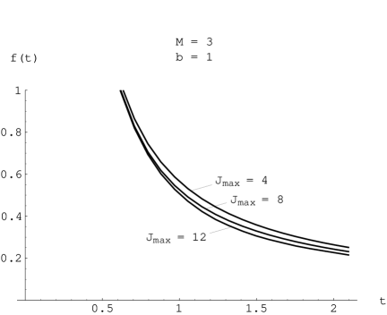
Figure 1: Plot of $f_{J_{\max}}(t)$ for $b=1$ and $J_{\max}=4,8,12$

appear consistent with this rate of convergence.

We can extrapolate to the limit $J_{\max}\rightarrow\infty$ using the asymptotic form

$$f_{J_{\max}}(t)=f_{\infty}(t)+J_{\max}^{-2}f^{(2)}(t)+\cdots.$$ (49)

For $b=0,0.5,1.0,3.0$ and $M=3$ we have calculated $f(t)$ using this extrapolation technique for $J_{\max}=10$ and 12. The results are shown in Figure 2.

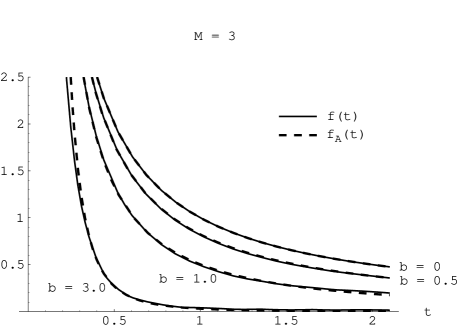
Figure 2: Plot of $f_{A}(t)$ and $f(t)$ for $b=0,.5,1,3$ and $M=3$

For comparison we have plotted the analytic solution

$$f_{A}(t)=(k(c)M)^{\frac{-2c^{2}}{1-c^{2}}}t^{\frac{-1-c^{2}}{1-c^{2}}}.$$ (50)

The relation between $b$ and $c$ can be found in (25) and (26).  The parameter $k(c)$ is fitted to the value of the correlator at the renormalization point $t=0.6.$ The agreement appears quite good.  Some deviations from the analytic solution are due to $O(\frac{1}{M^{2}t^{2}})$ residual terms, which were left out of the derivation of (50).  These effects are significant in the small $t$ region, $t\lesssim M^{-1}$, especially for larger values of $b$.  The values we find for $k(c)$ are shown in Table 2.

$$\overset{\text{Table 2}}{\begin{tabular}[c]{|l|l|l|l|}\hline\cr$b$&0.5&1.0&3.0\\ \hline\cr$k(c)$&1.77&1.77&1.68\\ \hline\cr\end{tabular}}$$

We can compare our results at small $b$ with a simple perturbative calculation. Evaluating the corresponding regulated two-loop diagram we obtain, for small $b$, $k(c)\approx 1.75$. This appears consistent with the results in Table 2.

6 Summary

We derived the angle-smeared spherical Hamiltonian for the massless Thirring model and constructed an explicit matrix representation. We discarded negligible high energy states using auxiliary cutoff parameters $J_{\max}$ and $K_{\max}$.  In this reduced space we computed the time evolution of quantum states and calculated the two-point correlator for several values of the coupling. The results of our computation are in close agreement with the known analytic solution.  In addition to demonstrating new computational methods, our analysis also serves as a consistency check of the regularization and renormalization methods introduced in [38].

We believe that this work represents a significant new direction in the non-perturbative computation of fermion dynamics.  Future work will study the application of these methods to systems of interacting bosons and fermions.

Chapter 3 Modal expansions and non-perturbative quantum field theory in Minkowski space

1 Introduction

Modal expansion methods have recently been used to study non-perturbative phenomena in quantum field theory [35, 36, 5, 38]. Modal field theory, the name for the general procedure, consists of two main parts. The first is to approximate field theory as a finite-dimensional quantum mechanical system. The second is to analyze the properties of the reduced system using one of several computational techniques.  The quantum mechanical approximation is generated by decomposing field configurations into free wave modes.  This technique has been explored using both spherical partial waves (spherical field theory [35, 36, 5, 38, 51]) and periodic box modes (periodic field theory [43]).

Having reduced field theory to a more tractable quantum mechanical system, we have several different ways to proceed.  Boson interactions in Euclidean space, for example, can be modeled using the method of diffusion Monte Carlo.  In many situations, however, Monte Carlo techniques are inadequate.  These include unquenched fermion systems, processes in Minkowski space, and the phenomenology of multi-particle states.  Difficulties arise when the functional integral measure cannot be treated as a probability distribution or when information must be extracted from excited states obscured by dominant lower lying states.  Fortunately there are several alternative methods in the modal field formalism which avoid these problems.  Matrix Runge-Kutta techniques were introduced in [51] as a method for calculating unquenched fermion interactions.  Here we discuss a different approach, one which directly calculates the spectrum and eigenstates of the Hamiltonian.  For this approach it is essential that the Hamiltonian is time-independent, and so we will consider periodic rather than spherical field theory.  As we demonstrate, these methods naturally accommodate the study of multi-particle states and Minkowskian dynamics.

We apply the spectral approach to $1+1$ dimensional $\phi^{4}$ theory in a periodic box and calculate the real and imaginary parts of the $\phi$ propagator.  Some interesting properties of $\phi_{2}^{4}$ theory such as the phase transition at large coupling were already discussed within the modal field formalism using Euclidean Monte Carlo techniques [43].  The purpose of this analysis is of a more general and exploratory nature.  Our aim is to test the viability of modal diagonalization techniques for quantum field Hamiltonians.  We would like to know whether we can clearly see multi-particle phenomena, the size of the errors and computational limitations with current computer resources, and how such methods might be extended to more complicated higher dimensional field theories.

The spectral method presented in the first part of our analysis is similar to the work of Brooks and Frautschi [27, 26], who considered a $1+1$ dimensional Yukawa model in a periodic box and deserves credit for the first application of diagonalization techniques using plane wave modes in a periodic box.  Our calculations are also similar in spirit to diagonalization-based Hamiltonian lattice formulations [23, 24] and Tamm-Dancoff light-cone and discrete light-cone quantization [47, 48, 2, 6].  There are, however, some differences which we should mention.  As in [27, 26] we are using a momentum lattice rather than a spatial lattice.  We find this convenient to separate out invariant subspaces according to total momentum quantum numbers.  Since we are using an equal time formulation our eigenvectors are not boost invariant as they would be on the light cone.  Also we are using a simple momentum cutoff scheme rather than a regularization scheme which includes Tamm-Dancoff Fock-space truncation.  As a result our renormalization procedure is relatively straightforward, but we will have to confront the problem of diagonalizing large Fock spaces from the very beginning.  In the latter part of the paper we mention current work on quasi-sparse eigenvector methods which can handle even exceptionally large Fock spaces.  Despite the differences among the various diagonalization approaches to field theory, the issues and problems discussed in our analysis are of a general nature.  We hope that the ideas presented here will be of use for the various different approaches.

2 Spectral method

The field configuration $\phi$ in $1+1$ dimensions is subject to periodic boundary conditions $\phi(t,x-L)=\phi(t,x+L).$  Expanding in terms of periodic box modes, we have

$$\phi(t,x)=\sqrt{\tfrac{1}{2L}}{\displaystyle\sum\limits_{n=0,\pm 1,...}}\phi_{n}(t)e^{in\pi x/L}.$$ (1)

The sum over momentum modes is regulated by choosing some large positive number $N_{\max}$ and throwing out all high-momentum modes $\phi_{n}$ such that $\left|n\right|>N_{\max}$. In this theory renormalization can be implemented by normal ordering the $\phi^{4}$ interaction term. After a straightforward calculation (details are given in [43]), we find that the counterterm Hamiltonian has the form

$$\tfrac{6\lambda b}{4!2L}{\displaystyle\sum\limits_{n=-N_{\max},N_{\max}}}\phi_{-n}\phi_{n},$$ (2)

where

$$b={\displaystyle\sum\limits_{n=-N_{\max},N_{\max}}}\tfrac{1}{2\omega_{n}},\qquad\omega_{n}=\sqrt{\tfrac{n^{2}\pi^{2}}{L^{2}}+\mu^{2}}.$$ (3)

We represent the canonical conjugate pair $\phi_{n}$ and $\frac{d\phi_{-n}}{dt}$ using the Schrödinger operators $q_{n}$ and $-i\tfrac{\partial}{\partial q_{n}}$.  Then the functional integral for $\phi^{4}$ theory is equivalent to that for a quantum mechanical system with Hamiltonian

$$H ={\displaystyle\sum\limits_{n=-N_{\max},N_{\max}}}\left[-\tfrac{1}{2}\tfrac{\partial}{\partial q_{-n}}\tfrac{\partial}{\partial q_{n}}+\tfrac{1}{2}(\omega_{n}^{2}-\tfrac{\lambda b}{4L})q_{-n}q_{n}\right]$$ (4)

$$+\tfrac{\lambda}{4!2L}{\displaystyle\sum\limits_{\genfrac{}{}{0.0pt}{1}{n_{i}=-N_{\max},N_{\max}}{n_{1}+n_{2}+n_{3}+n_{4}=0}}}q_{n_{1}}q_{n_{2}}q_{n_{3}}q_{n_{4}}.$$

We now consider the Hilbert space of our quantum mechanical system.  Given $d$, an array of non-negative integers,

$$d=\left\{d_{-N_{\max}},\cdots d_{N_{\max}}\right\},$$ (5)

we denote $p_{d}(q)$ as the following monomial with total degree $\left|d\right|$,

$$p_{d}(q)={\displaystyle\prod\limits_{n=-N_{\max},N_{\max}}}q_{n}^{d_{n}},\qquad{\displaystyle\sum\limits_{n}}d_{n}=\left|d\right|.$$ (6)

We define $G_{\zeta}(q)$ to be a Gaussian of the form

$$G_{\zeta}(q)={\displaystyle\prod\limits_{n=-N_{\max},N_{\max}}}\exp\left[-\tfrac{q_{-n}q_{n}\sqrt{\zeta^{2}+n^{2}\pi^{2}/L^{2}}}{2}\right].$$ (7)

$\zeta$ is an adjustable parameter which we will set later.  Any square-integrable function $\psi(q)$ can be written as a superposition

$$\psi(q)={\displaystyle\sum\limits_{d}}c_{d}\,p_{d}(q)G_{\zeta}(q).$$ (8)

In this analysis we consider only the zero-momentum subspace.  We impose this constraint by restricting the sum in (8) to monomials satisfying

$${\displaystyle\sum\limits_{n}}nd_{n}=0.$$ (9)

We will restrict the space of functions $\psi(q)$ further by removing high energy states in the following manner.  Let

$$k(d)={\displaystyle\sum_{n}}\left|n\right|d_{n}.$$ (10)

$k(d)$ was first introduced in [51] and provides an estimate of the kinetic energy associated with a given state. Let us define two auxiliary cutoff parameters, $K_{\max}$ and $D_{\max}$.  We restrict the sum in (8) to monomials such that $k(d)<K_{\max}$ and $\left|d\right|\leq D_{\max}$.  We will refer to the corresponding subspace as $V_{K_{\max},D_{\max}}$.  The cutoff $K_{\max}$ removes states with high kinetic energy and the cutoff $D_{\max}$ eliminates states with a large number of excited modes.  We should stress that $K_{\max}$ and $D_{\max}$ are only auxiliary cutoffs.  We increase these parameters until the physical results appear close to the asymptotic limit $K_{\max},D_{\max}\rightarrow\infty$.  In our scheme ultraviolet regularization is provided only by the momentum cutoff parameter $N_{\max}$.

Our plan is to analyze the spectrum and eigenstates of $H$ restricted to this approximate low energy subspace, $V_{K_{\max},D_{\max}}$. For any fixed $L$ and $N_{\max}$, $H$ is the Hamiltonian for a finite-dimensional quantum mechanical system and the results should converge in the limit $K_{\max},D_{\max}\rightarrow\infty$.  We obtain the desired field theory result by then taking the limit $L,\frac{N_{\max}}{L}\rightarrow\infty$.

3 Results

We have calculated the matrix elements of $H$ restricted to $V_{K_{\max},D_{\max}}$ using a symbolic differentiation-integration algorithm and diagonalized $H$, obtaining both eigenvalues and eigenstates.  Let $\Delta$ be the full propagator,

$$\Delta(p^{2})=i\int d^{2}x\,e^{ip_{\nu}x^{\nu}}\left\langle 0\right|T\left[\phi(x^{\mu})\phi(0)\right]\left|0\right\rangle.$$ (11)

We have computed $\Delta$ by inserting our complete set of eigenstates (complete in $V_{K_{\max},D_{\max}}$).  Let $\Delta_{\text{mp}}$ be the multi-particle contribution to $\Delta$,

$$\Delta_{\text{mp}}(p^{2})=\Delta(p^{2})-\Delta_{\text{pole}}(p^{2}),$$ (12)

where $\Delta_{\text{pole}}$ is the single-particle pole contribution.  We are primarily interested in $\Delta_{\text{mp}}$, a quantity that cannot be obtained for $p^{2}>0$ using Monte Carlo methods.  Since the imaginary part of $\Delta_{\text{pole}}$ is a delta function, it is easy to distinguish the single-particle and multi-particle contributions in a plot of the imaginary part of $\Delta$.  The real part of $\Delta$, however, is dominated by the one-particle pole.  For this reason we have chosen to plot the real part of $\Delta_{\text{mp}}$ rather than that of $\Delta$.

Although we have referred to multi-particle states, it should be noted that in our finite periodic box there are no true continuum multi-particle states.  Instead we find densely packed discrete spectra with level separation of size $\sim L^{-1}$ which become continuum states in the limit $L\rightarrow\infty$.  We can approximate the contribution of these $L\rightarrow\infty$ continuum states by a simple smoothing process. We included a small width $\Gamma\sim L^{-1}$ to each of the would-be continuum states and averaged over a range of values for $L$.  For the results we report here we have averaged over values $L=2.0\pi,2.1\pi,\cdots 2.8\pi.$  For convenience all units have been scaled such that $\mu=1$.

The parameter $\zeta$ was adjusted to reduce the errors due to the finite cutoff values $K_{\max}$ and $D_{\max}$.  Since the spectrum of $H$ is bounded below, errors due to finite $K_{\max}$ and $D_{\max}$ generally drive the estimated eigenvalues higher.  One strategy, therefore, is to optimize $\zeta$ by minimizing the trace of $H$ restricted to the subspace $V_{K_{\max},D_{\max}}$.  The approach used here is a slight variation of this — we have minimized the trace of $H$ restricted to a smaller subspace $V_{K_{\max}^{\prime},D_{\max}^{\prime}}\subset V_{K_{\max},D_{\max}}$.  The aim is to accelerate the convergence of the lowest energy states rather than the entire space $V_{K_{\max},D_{\max}}$.  Throughout our analysis we used $K_{\max}^{\prime},D_{\max}^{\prime}=8,3.$

For $\frac{\lambda}{4!}=0.50$ we have plotted the imaginary part of $\Delta$ in Figure 1

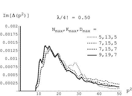
Figure 1: Imaginary part of $\Delta(p^{2})$ for $\frac{\lambda}{4!}=0.50$ and several values for $N_{\max},K_{\max},D_{\max}$

and the real part of $\Delta_{\text{mp}}$ in Figure 2.

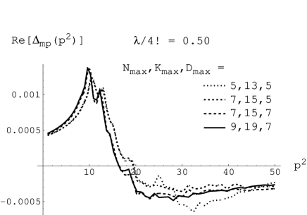
Figure 2: Real part of $\Delta_{\text{mp}}(p^{2})$ for $\frac{\lambda}{4!}=0.50$ and several values for $N_{\max},K_{\max},D_{\max}$

The value $\frac{\lambda}{4!}=0.50$ is above the threshold for reliable perturbative approximation ($\frac{\lambda}{4!}\lesssim 0.25$) but below the critical value at which $\phi\rightarrow-\phi$ symmetry breaks spontaneously ($\frac{\lambda}{4!}\approx 2.5).$  The contribution of the one-particle state appears near $p^{2}=(0.93)^{2}$ and the three-particle threshold is at approximately $p^{2}=(2.9)^{2}$.  We have chosen several different values for $N_{\max},K_{\max},D_{\max}$ to show the convergence as these parameters become large.  The plot for $N_{\max},K_{\max},D_{\max}=9,19,7$ appears relatively close to the asymptotic limit.  The somewhat bumpy texture of the curves is due to the finite size of our periodic box and diminishes with increasing $L$.  From dimensional power counting, we expect errors for finite $N_{\max}$ to scale as $N_{\max}^{-2}$.  Assuming that $K_{\max}$ and $D_{\max}$ also function as uniform energy cutoffs, we expect a similar error dependence – and it appears plausible from the results in Figures 1 and 2.  A more systematic analysis of the errors and extrapolation methods for finite $N_{\max},K_{\max},D_{\max}$, and $L,$ will be discussed in future work.

In Figures 3 and 4

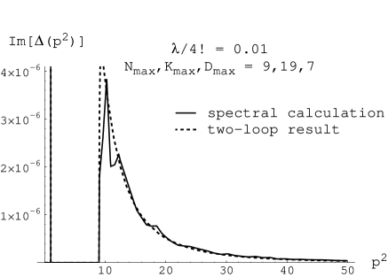
Figure 3: Imaginary part of $\Delta(p^{2})$ for $\frac{\lambda}{4!}=0.01$ and comparison with the two-loop result

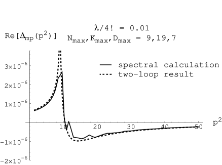
Figure 4: Real part of $\Delta_{\text{mp}}(p^{2})$ for $\frac{\lambda}{4!}=0.01$ and comparison with the two-loop result

we have compared our spectral calculations with the two-loop perturbative result for $\frac{\lambda}{4!}=0.01$.  We have used $N_{\max},K_{\max},D_{\max}=9,19,7$, and the agreement appears good.  For small $\frac{\lambda}{4!}$ the propagator has a very prominent logarithmic cusp at the three-particle threshold, which can be seen clearly in Figures 3 and 4.

In Figures 5 and 6

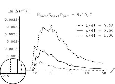
Figure 5: Imaginary part of $\Delta(p^{2})$ for $\frac{\lambda}{4!}=0.25,0.50,1.00$

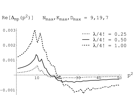
Figure 6: Real part of $\Delta_{\text{mp}}(p^{2})$ for $\frac{\lambda}{4!}=0.25,0.50,1.00$

we have compared results for $\frac{\lambda}{4!}=0.25$, $0.50$, $1.00$.  We have again used $N_{\max},K_{\max},D_{\max}=9,19,7$.  In contrast with the quadratic scaling in the perturbative regime, the results here scale approximately linearly with $\frac{\lambda}{4!}$.  An interesting and perhaps related observation is that the magnitude of the multi-particle contribution to $\Delta$ remains small $(\lesssim 0.003$) even for the rather large coupling value $\frac{\lambda}{4!}=1.00$.

4 Limitations and new ideas

We now address the computational limits of the diagonalization techniques presented in this work.  These techniques are rather straightforward and can in principle be generalized to any field theory.  In practise however the Fock space $V_{K_{\max},D_{\max}}$ becomes prohibitively large, especially for higher dimensional theories.  The data in Figures 1 and 2 and crosschecks with Euclidean Monte Carlo results suggest that for $N_{\max}=9\$and $L=2.0\pi,\cdots 2.8\pi$ our spectral results with $K_{\max},D_{\max}=19,7$ and $\frac{\lambda}{4!}<1$ are within 20% of the $K_{\max},D_{\max}\rightarrow\infty$ limit.   In this case $V_{K_{\max},D_{\max}}$ is a $2036$ dimensional space and requires about 100 MB of RAM using general (dense) matrix methods.

Sparse matrix techniques such as the Lanczos or Arnoldi schemes allow us to push the dimension of the Fock space to about 10⁵ states.  This may be sufficient to do accurate calculations near the critical point $\frac{\lambda}{4!}\approx 2.5$ for larger values of $L$ and $N_{\max}.$  It is, however, near the upper limit of what is possible using current computer technology and existing algorithms.  Unfortunately field theories in $2+1$ and $3+1$ dimensions will require much larger Fock spaces, probably at least 10¹² and 10¹⁸ states respectively.  In order to tackle these larger Fock spaces it is necessary to venture beyond standard diagonalization approaches.  The problem of large Fock spaces ($\gg$10⁶ states) is beyond the intended scope of this analysis.  But since it is of central importance to the diagonalization approach to field theory we would like to briefly comment on current work being done which may resolve many of the difficulties.  The new approach takes advantage of the sparsity of the Fock-space Hamiltonian and the approximate (quasi-)sparsity of the eigenvectors.  A detailed description will be provided in a future publication [39].

We start with some observations about the eigenvectors of the $\phi_{1+1}^{4}$ Hamiltonian for $N_{\max}=9,$ $L=2.5\pi$ and $K_{\max},D_{\max}=19,7.$  To make certain that we are probing non-perturbative physics we will set $\frac{\lambda}{4!}=2.5,$ the approximate critical point value.  We label the normalized eigenvectors as $\left|v_{0}\right\rangle$, $\left|v_{1}\right\rangle$,$\cdots,$ ascending in order with respect to energy.  We also define $\left|b_{0}\right\rangle$, $\left|b_{1}\right\rangle$,$\cdots$ as the normalized eigenvectors of the free, non-interacting theory.  For any $v_{i}$ we know

$$\sum_{j}\left|\left\langle b_{j}|v_{i}\right\rangle\right|^{2}=1.$$ (13)

Let us define $\left\|\left|v_{i}\right\rangle\right\|_{(n)}$ as the partial sum

$$\left\|\left|v_{i}\right\rangle\right\|_{(n)}=\sum_{k=1,\cdots n}\left|\left\langle b_{j_{k}}|v_{i}\right\rangle\right|^{2},$$ (14)

where the inner products have been sorted from largest to smallest

$$\left|\left\langle b_{j_{1}}|v_{i}\right\rangle\right|\geq\left|\left\langle b_{j_{2}}|v_{i}\right\rangle\right|\geq\cdots.$$ (15)

Table 1 shows $\left\|\left|v_{i}\right\rangle\right\|_{(n)}$ for several eigenvectors and different values of $n$.

|v0⟩0.750.840.900.94|v1⟩0.890.920.950.97|v5⟩0.870.910.940.96|v10⟩0.770.860.900.94Table 1Table 1missing-subexpressionfragments fragments|v0⟩0.750.840.900.94fragments|v1⟩0.890.920.950.97fragments|v5⟩0.870.910.940.96fragments|v10⟩0.770.860.900.94\overset{\text{Table 1}}{\begin{array}[c]{c}\\ \begin{tabular}[c]{l|l|l|l|l|}$\left\|\left|v_{i}\right\rangle\right\|_{(n)}$&$n=10$&$n=20$&$n=40$&$n=80$\\ \hline\cr$\left|v_{0}\right\rangle$&0.75&0.84&0.90&0.94\\ \hline\cr$\left|v_{1}\right\rangle$&0.89&0.92&0.95&0.97\\ \hline\cr$\left|v_{5}\right\rangle$&0.87&0.91&0.94&0.96\\ \hline\cr$\left|v_{10}\right\rangle$&0.77&0.86&0.90&0.94\\ \hline\cr\end{tabular}\end{array}}

‖|vi⟩‖(n)=n10=n20=n40=n80‖|vi⟩‖(n)=n10=n20=n40=n80

Despite the non-perturbative coupling and complex phenomena associated with the phase transition, we see from the table that each of the eigenvectors can be approximated by just a small number of its largest Fock-space components.  We recall that the Fock space for this system has 2036 dimensions.  The eigenvectors are therefore quasi-sparse in this space, a consequence of the sparsity of the Hamiltonian.  If we write the Hamiltonian as a matrix in the free Fock-space basis, a typical row or column contains only about 200 non-zero entries, a number we refer to as $N_{\text{transition}}.$  In [39] we show that a typical eigenvector will be dominated by the largest $\sqrt{N_{\text{transition}}}$ elements.  The key point is that $\sqrt{N_{\text{transition}}}$ is quite manageable — on the order of $10^{3}$ and 10⁵ for $2+1$ and $3+1$ dimensional field theories respectively.  Although the size of the Fock space for these systems are enormous, the extreme sparsity of the Hamiltonian suggests that the eigenvectors can be approximated using current computational resources.

With this simplification, the task is to find the important basis states for a given eigenvector.  Since the important basis states for one eigenvector are generally different from that of another, each eigenvector is determined independently.  This provides a starting point for parallelization, and many eigenvectors can be determined at the same time using massively parallel computers.  In [39] we present a simple stochastic algorithm where the exact eigenvectors act as stable fixed points of the update process.

5 Summary

We have introduced a spectral approach to periodic field theory and used it to calculate the propagator in $1+1$ dimensional $\phi^{4}$ theory.  We find that the straightforward application of these methods with existing computer technology can be useful for describing the multi-particle properties of the theory, information difficult to obtain using Euclidean Monte Carlo methods.  However the extension to higher dimensional theories is made difficult by the large size of the corresponding Fock space.  As a possible solution to this problem, we note that each eigenvector of the $\phi_{1+1}^{4}$ Hamiltonian can be well-approximated using relatively few components and discuss some current work on quasi-sparse eigenvector methods.

Chapter 4 Quasi sparse methods in the diagonalization of quantum field Hamiltonians

1 Introduction

Most computational work in non-perturbative quantum field theory and many body phenomena rely on one of two general techniques, Monte Carlo or diagonalization.  These methods are nearly opposite in their strengths and weaknesses.  Monte Carlo requires relatively little storage, can be performed using parallel processors, and in some cases the computational effort scales reasonably with system size.  But it has great difficulty for systems with sign or phase oscillations and provides only indirect information on wavefunctions and excited states.  In contrast diagonalization methods do not suffer from fermion sign problems, can handle complex-valued actions, and can extract details of the spectrum and eigenstate wavefunctions.  However the main problem with diagonalization is that the required memory and CPU time scales exponentially with the size of the system.

In view of the complementary nature of the two methods, we consider the combination of both diagonalization and Monte Carlo within a computational scheme.  We propose a new approach which takes advantage of the strengths of the two computational methods in their respective domains.  The first half of the method involves finding and diagonalizing the Hamiltonian restricted to an optimal subspace.  This subspace is designed to include the most important basis vectors of the lowest energy eigenstates.  Once the most important basis vectors are found and their interactions treated exactly, Monte Carlo is used to sample the contribution of the remaining basis vectors.  By this two-step procedure much of the sign problem is negated by treating the interactions of the most important basis states exactly, while storage and CPU problems are resolved by stochastically sampling the collective effect of the remaining states.

In our approach diagonalization is used as the starting point of the Monte Carlo calculation.  Therefore the two methods should not only be efficient but work well together.  On the diagonalization side there are several existing methods using Tamm-Dancoff truncation [47], similarity transformations [17, 18], density matrix renormalization group [60, 61], or variational algorithms such as stochastic diagonalization [25, 10].  However we find that each of these methods is either not sufficiently general, not able to search an infinite or large dimensional Hilbert space, not efficient at finding important basis vectors, or not compatible with the subsequent Monte Carlo part of the calculation.  The Monte Carlo part of our diagonalization/Monte Carlo scheme is discussed separately in a companion paper [40].  In this paper we consider the diagonalization part of the scheme.  We introduce a new diagonalization method called quasi-sparse eigenvector (QSE) diagonalization.  It is a general algorithm which can operate using any basis, either orthogonal or non-orthogonal, and any sparse Hamiltonian, either real, complex, Hermitian, non-Hermitian, finite-dimensional, or infinite-dimensional.  It is able to find the most important basis states of several low energy eigenvectors simultaneously, including those with identical quantum numbers, from a random start with no prior knowledge about the form of the eigenvectors.

Our discussion is organized as follows.  We first define the notion of quasi-sparsity in eigenvectors and introduce the quasi-sparse eigenvector method.  We discuss when the low energy eigenvectors are likely to be quasi-sparse and make an analogy with Anderson localization.  We then consider three examples which test the performance of the algorithm.  In the first example we find the lowest energy eigenstates for a random sparse real symmetric matrix.  In the second example we find the lowest eigenstates sorted according to the real part of the eigenvalue for a random sparse complex non-Hermitian matrix.  In the last example we consider the case of an infinite-dimensional Hamiltonian defined by $1+1$ dimensional $\phi^{4}$ theory in a periodic box.  We conclude with a summary and some comments on the role of quasi-sparse eigenvector diagonalization within the context of the new diagonalization/Monte Carlo approach.

2 Quasi-sparse eigenvector method

Let $\left|e_{i}\right\rangle$ denote a complete set of basis vectors.  For a given energy eigenstate

$$|v\rangle=\sum_{i}c_{i}\left|e_{i}\right\rangle,$$ (1)

we define the important basis states of $|v\rangle$ to be those $\left|e_{i}\right\rangle$ such that for fixed normalizations of $|v\rangle$ and the basis states, $\left|c_{i}\right|$ exceeds a prescribed threshold value.  If $|v\rangle$ can be well-approximated by the contribution from only its important basis states we refer to the eigenvector $|v\rangle$ as quasi-sparse with respect to $\left|e_{i}\right\rangle$.

Standard sparse matrix algorithms such as the Lanczos or Arnoldi methods allow one to find the extreme eigenvalues and eigenvectors of a sparse matrix efficiently, without having to store or manipulate large non-sparse matrices.  However in quantum field theory or many body theory one considers very large or infinite dimensional spaces where even storing the components of a general vector is impossible.  For these more difficult problems the strategy is to approximate the low energy eigenvectors of the large space by diagonalizing smaller subspaces.  If one has sufficient intuition about the low energy eigenstates it may be possible to find a useful truncation of the full vector space to an appropriate smaller subspace.  In most cases, however, not enough is known a priori about the low energy eigenvectors.  The dilemma is that to find the low energy eigenstates one must truncate the vector space, but in order to truncate the space something must be known about the low energy states.

Our solution to this puzzle is to find the low energy eigenstates and the appropriate subspace truncation at the same time by a recursive process.  We call the method quasi-sparse eigenvector (QSE) diagonalization, and we describe the steps of the algorithm as follows.  The starting point is any complete basis for which the Hamiltonian matrix $H_{ij}$ is sparse.  The basis vectors may be non-orthogonal and/or the Hamiltonian matrix may be non-Hermitian.  The following steps are now iterated:

1. Select a subset of basis vectors $\left\{e_{i_{1}},\cdots,e_{i_{n}}\right\}$ and call the corresponding subspace $S$.

2. Diagonalize $H$ restricted to $S$ and find one eigenvector $v$.

3. Sort the basis components of $v$ according to their magnitude and remove the least important basis vectors.

4. Replace the discarded basis vectors by new basis vectors.  These are selected at random according to some weighting function from a pool of candidate basis vectors which are connected to the old basis vectors through non-vanishing matrix elements of $H$.

5. Redefine $S$ as the subspace spanned by the updated set of basis vectors and repeat steps 2 through 5.

If the subset of basis vectors is sufficiently large, the exact low energy eigenvectors will be stable fixed points of the QSE update process.  We can show this as follows.  Let $\left|i\right\rangle$ be the eigenvectors of the submatrix of $H$ restricted to the subspace $S$, where $S$ is the span of the subset of basis vectors after step 3 of the QSE algorithm.  Let $\left|A_{j}\right\rangle$ be the remaining basis vectors in the full space not contained in $S$.  We can represent $H$ as

$$\left[\begin{array}[c]{cccccc}\lambda_{1}&0&\cdots&\left\langle 1\right|H\left|A_{1}\right\rangle&\left\langle 1\right|H\left|A_{2}\right\rangle&\cdots\\ 0&\lambda_{2}&\cdots&\left\langle 2\right|H\left|A_{1}\right\rangle&\left\langle 2\right|H\left|A_{2}\right\rangle&\cdots\\ \vdots&\vdots&\ddots&\vdots&\vdots&\cdots\\ \left\langle A_{1}\right|H\left|1\right\rangle&\left\langle A_{1}\right|H\left|2\right\rangle&\cdots&E\cdot\lambda_{A_{1}}&\left\langle A_{1}\right|H\left|A_{2}\right\rangle&\cdots\\ \left\langle A_{2}\right|H\left|1\right\rangle&\left\langle A_{2}\right|H\left|2\right\rangle&\cdots&\left\langle A_{2}\right|H\left|A_{1}\right\rangle&E\cdot\lambda_{A_{2}}&\cdots\\ \vdots&\vdots&\vdots&\vdots&\vdots&\ddots\end{array}\right].$$ (2)

We have used Dirac’s bra-ket notation to represent the terms of the Hamiltonian matrix.  In cases where the basis is non-orthogonal and/or the Hamiltonian is non-Hermitian, the meaning of this notation may not be clear.  When writing $\left\langle A_{1}\right|H\left|1\right\rangle$, for example, we mean the result of the dual vector to $\left|A_{1}\right\rangle$ acting upon the vector $H\left|1\right\rangle$.  In (2) we have written the diagonal terms for the basis vectors $\left|A_{j}\right\rangle$ with an explicit factor $E$.  We let $\left|1\right\rangle$ be the approximate eigenvector of interest and have shifted the diagonal entries so that $\lambda_{1}=0.$  Our starting hypothesis is that $\left|1\right\rangle$ is close to some exact eigenvector of $H$ which we denote as $\left|1_{\text{full}}\right\rangle$.  More precisely we assume that the components of $\left|1_{\text{full}}\right\rangle$ outside $S$ are small enough so that we can expand in inverse powers of the introduced parameter $E.$

We now expand the eigenvector as

$$\left|1_{\text{full}}\right\rangle=\left[\begin{array}[c]{c}1\\ c_{2}^{\prime}E^{-1}+\cdots\\ \vdots\\ c_{A_{1}}^{\prime}E^{-1}+\cdots\\ c_{A_{2}}^{\prime}E^{-1}+\cdots\\ \vdots\end{array}\right]$$ (3)

and the corresponding eigenvalue as

$$\lambda_{\text{full}}=\lambda_{1}^{\prime}E^{-1}+\cdots.$$ (4)

In (3) we have chosen the normalization of $\left|1_{\text{full}}\right\rangle$ such that $\left\langle 1\right.\left|1_{\text{full}}\right\rangle=1$.  From the eigenvalue equation

$$H\left|1_{\text{full}}\right\rangle=\lambda_{\text{full}}\left|1_{\text{full}}\right\rangle$$ (5)

we find at lowest order

$$c_{A_{j}}^{\prime}=-\tfrac{\left\langle A_{j}\right|H\left|1\right\rangle}{\lambda_{A_{j}}}.$$ (6)

We see that at lowest order the component of $\left|1_{\text{full}}\right\rangle$ in the $\left|A_{j}\right\rangle$ direction is independent of the other vectors $\left|A_{j^{\prime}}\right\rangle$.  If $\left|1\right\rangle$ is sufficiently close to $\left|1_{\text{full}}\right\rangle$ then the limitation that only a fixed number of new basis vectors is added in step 4 of the QSE algorithm is not relevant.  At lowest order in $E^{-1}$ the comparison of basis components in step 3 (in the next iteration) is the same as if we had included all remaining vectors $\left|A_{j}\right\rangle$ at once.  Therefore at each update only the truly largest components are kept and the algorithm converges to some optimal approximation of $\left|1_{\text{full}}\right\rangle$.  This is consistent with the actual performance of the algorithm as we will see in some examples later.  In those examples we also demonstrate that the QSE algorithm is able to find several low energy eigenvectors simultaneously.  The only change is that when diagonalizing the subspace $S$ we find more than one eigenvector and apply steps 3 and 4 of the algorithm to each of the eigenvectors.

3 Quasi-sparsity and Anderson localization

As the name indicates the accuracy of the quasi-sparse eigenvector method depends on the quasi-sparsity of the low energy eigenstates in the chosen basis.  If the eigenvectors are quasi-sparse then the QSE method provides an efficient way to find the important basis vectors.  In the context of our diagonalization/Monte Carlo approach, this means that diagonalization does most of the work and only a small amount of correction is needed.  This correction is found by Monte Carlo sampling the remaining basis vectors, a technique called stochastic error correction [40].  If however the eigenvectors are not quasi-sparse then one must rely more heavily on the Monte Carlo portion of the calculation.

The fastest and most reliable way we know to determine whether the low energy eigenstates of a Hamiltonian are quasi-sparse with respect to a chosen basis is to use the QSE algorithm and look at the results of the successive iterations.  But it is also useful to consider the question more intuitively, and so we consider the following example.

Let $H$ be a sparse Hermitian $2000\times 2000$ matrix defined by

$$H_{jk}=\log(j)\cdot\delta_{jk}+x_{jk}\cdot M_{jk},$$ (7)

where $j$ and $k$ run from $1$ to $2000$, $x_{jk}$ is a Gaussian random real variable centered at zero with standard deviation $x_{\text{rms}}=0.25$, and $M_{jk}$ is a sparse symmetric matrix consisting of random $0$’s and $1$’s such that the density of $1$’s is $5\%$.  The reason for introducing the $\log(j)$ term in the diagonal is to produce a large variation in the density of states. With this choice the density of states increases exponentially with energy.  Our test matrix is small enough that all eigenvectors can be found without difficulty.  We will consider the distribution of basis components for the eigenvectors of $H$.  In Figure 1

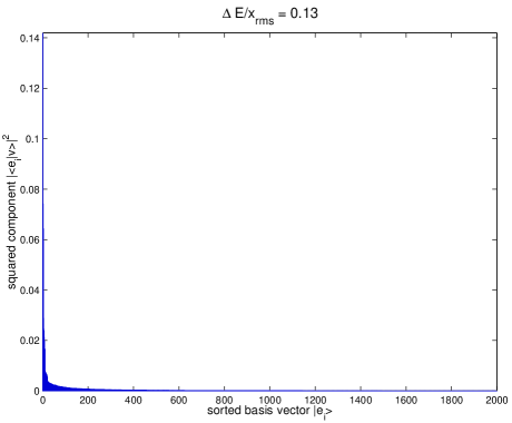
Figure 1: Distribution of basis components for an eigenvector where the spacing between consecutive levels is $\Delta E=0.13x_{\text{rms}}$.

we show the square of the basis components for a given low energy eigenvector $\left|v\right\rangle.$  The basis components are sorted in order of descending importance.  The ratio of $\Delta E$, the average spacing between neighboring energy levels, to $x_{\text{rms}}$ is $0.13$.  We see that the eigenvector is dominated by a few of its most important basis components.  In Figure 2

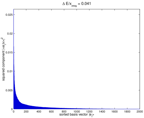
Figure 2: Distribution of basis components for an eigenvector where $\Delta E=0.041x_{\text{rms}}$.

we show the same plot for another eigenstate but one where the spacing between levels is three times smaller, $\Delta E/x_{\text{rms}}=0.041.$  This eigenvector is not nearly as quasi-sparse.  The effect is even stronger in Figure 3,

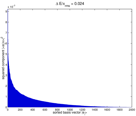
Figure 3: Distribution of basis components for an eigenvector where $\Delta E=0.024x_{\text{rms}}$.

where we show an eigenvector such that the spacing between levels is $\Delta E/x_{\text{rms}}=0.024$.

Our observations show a strong effect of the density of states on the quasi-sparsity of the eigenvectors.  States with a smaller spacing between neighboring levels tend to have basis components that extend throughout the entire space, while states with a larger spacing tend to be quasi-sparse.  The relationship between extended versus localized eigenstates and the density of states has been studied in the context of Anderson localization and metal-insulator transitions [3, 56, 63, 28]. The simplest example is the tight-binding model for a single electron on a one-dimensional lattice with $Z$ sites,

$$H=\sum_{j}d_{j}\left|j\right\rangle\left\langle j\right|+\sum_{\left\langle jj^{\prime}\right\rangle}t_{jj^{\prime}}\left|j\right\rangle\left\langle j^{\prime}\right|.$$ (8)

$\left|j\right\rangle$ denotes the atomic orbital state at site $j,$ $d_{j}$ is the on-site potential, and $t_{jj^{\prime}}$ is the hopping term between nearest neighbor sites $j$ and $j^{\prime}$.  If both terms are uniform ($d_{j}=d,$ $t_{jj^{\prime}}=t$) then the eigenvalues and eigenvectors of $H$ are

$$Hv_{n} =(d+2t\cos\tfrac{2\pi n}{Z})v_{n},$$ (9)

$$v_{n} =\tfrac{1}{\sqrt{Z}}\sum_{j}e^{i\tfrac{2\pi nj}{Z}}\left|j\right\rangle,$$ (10)

where $n=1,\cdots,Z$ labels the eigenvectors.  In the absence of diagonal and off-diagonal disorder, the eigenstates of $H$ extend throughout the entire lattice.  The eigenvalues are also approximately degenerate, all lying within an interval of size 4$t$.  However, if diagonal and/or off-diagonal disorder is introduced, the eigenvalue spectrum becomes less degenerate.  If the disorder is sufficiently large, the eigenstates become localized to only a few neighboring lattice sites giving rise to a transition of the material from metal to insulator.

We can regard a sparse quantum Hamiltonian as a similar type of system, one with both diagonal and general off-diagonal disorder.  If the disorder is sufficient such that the eigenvalues become non-degenerate, then the eigenvectors will be quasi-sparse.  We reiterate that the most reliable way to determine if the low energy states are quasi-sparse is to use the QSE algorithm.  Intuitively, though, we expect the eigenstates to be quasi-sparse with respect to a chosen basis if the spacing between energy levels is not too small compared with the size of the off-diagonal entries of the Hamiltonian matrix.

4 Finite matrix examples

As a first test of the QSE method, we will find the lowest four energy states of the random symmetric matrix $H$ defined in (7).  So that there is no misunderstanding, we should repeat that diagonalizing a $2000\times 2000$ matrix is not difficult.  The purpose of this test is to analyze the performance of the method in a controlled environment.  One interesting twist is that the algorithm uses only small pieces of the matrix and operates under the assumption that the space may be infinite dimensional.  A sample MATLAB program similar to the one used here has been printed out as a tutorial example in [34].

The program starts from a random configuration, 70 basis states for each of the four eigenvectors.  With each iteration we select $10$ replacement basis states for each of the eigenvectors.  In Figure 4

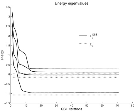
Figure 4: Comparison of the four lowest exact energies $E_{i}$ and QSE results $E_{i}^{\text{QSE}}$ as functions of iteration number.

we show the exact energies and the results of the QSE method as functions of iteration number.  In Figure 5

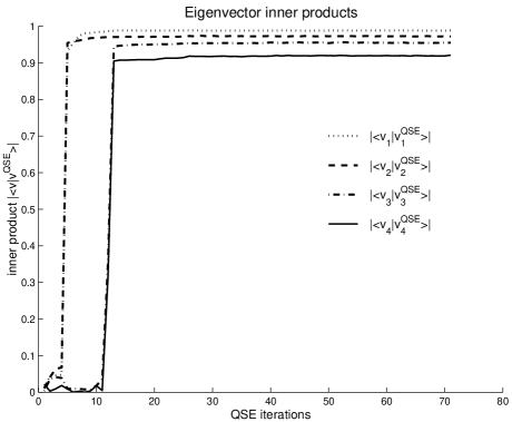
Figure 5: Inner products between the normalized exact eigenvectors $\left|v_{i}\right\rangle$ and the QSE results $\left|v_{i}^{\text{QSE}}\right\rangle$ as functions of iteration number.

we show the inner products of the normalized QSE eigenvectors with the normalized exact eigenvectors.  We note that all of the eigenvectors were found after about 15 iterations and remained stable throughout successive iterations.  Errors are at the $5$ to $10\%$ level, which is about the theoretical limit one can achieve using this number of basis states.  The QSE method has little difficulty finding several low lying eigenvectors simultaneously because it uses the distribution of basis components for each of the eigenvectors to determine the update process.  This provides a performance advantage over variational-based techniques such as stochastic diagonalization in finding eigenstates other than the ground state.

As a second test we consider a sparse non-Hermitian matrix with complex eigenvalues.  This type of matrix is not amenable to variational-based methods.  We will find the four eigenstates corresponding with eigenvalues with the lowest real part for the random complex non-Hermitian matrix

$$H_{jk}^{\prime}=(1+i\cdot c_{jk})H_{jk}.$$ (11)

$H_{jk}$ is the same matrix used previously and$\ c_{jk}$ is a uniform random variable distributed between $-1$ and 1.  As before the program is started from a random configuration, 70 basis states for each of the four eigenvectors.  For each iteration $10$ replacement basis vectors are selected for each of the eigenvectors.  In Figure 6

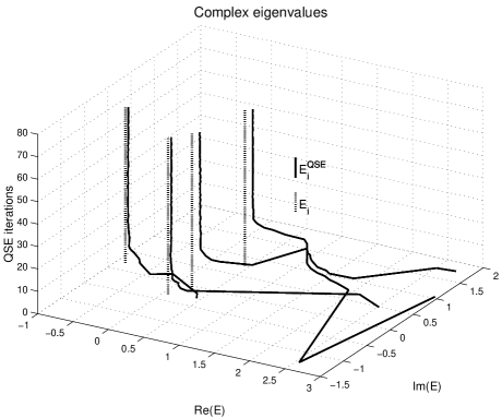
Figure 6: Comparison of the four lowest exact eigenvalues $E_{i}$ (sorted by real part) and QSE results $E_{i}^{\text{QSE}}$ in the complex plane as functions of iteration number.

the exact eigenvalues and the results of the QSE run are shown in the complex plane as functions of iteration number.  In Figure 7

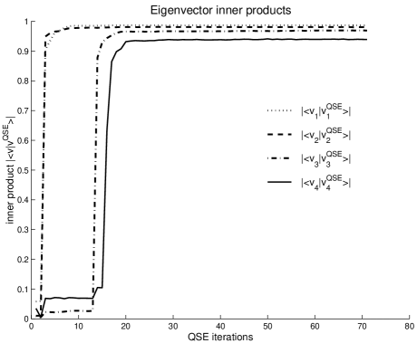
Figure 7: Inner products between the normalized exact eigenvectors $\left|v_{i}\right\rangle$ and the QSE results $\left|v_{i}^{\text{QSE}}\right\rangle$ as functions of iteration number.

we show the inner products of the QSE eigenvectors with the exact eigenvectors.  All of the eigenvectors were found after about 20 iterations and remained stable throughout successive iterations.  Errors were again at about the $5$ to $10\%$ level.

5 $\phi^{4}$ theory in $1+1$ dimensions

We now apply the QSE method to an infinite dimensional quantum Hamiltonian.  We consider $\phi^{4}$ theory in $1+1$ dimensions, a system that is familiar to us from previous studies using Monte Carlo [43] and explicit diagonalization [52].  The Hamiltonian density for $\phi^{4}$ theory in $1+1$ dimensions has the form

$$\mathcal{H}=\tfrac{1}{2}\left(\tfrac{\partial\phi}{\partial t}\right)^{2}+\tfrac{1}{2}\left(\tfrac{\partial\phi}{\partial x}\right)^{2}+\tfrac{\mu^{2}}{2}\phi^{2}+\tfrac{\lambda}{4!}\text{:}\phi^{4}\text{:},$$

where the normal ordering is with respect to the mass $\mu$.  We consider the system in a periodic box of length $2L$.  We then expand in momentum modes and reinterpret the problem as an equivalent Schrödinger equation [43].  The resulting Hamiltonian is

$$H =-\tfrac{1}{2}{\displaystyle\sum_{n}}\tfrac{\partial}{\partial q_{-n}}\tfrac{\partial}{\partial q_{n}}+\tfrac{1}{2}{\displaystyle\sum_{n}}\left(\omega_{n}^{2}(\mu)-\tfrac{\lambda b(\mu)}{8L}\right)\,q_{-n}q_{n}$$ (12)

$$+\tfrac{\lambda}{4!2L}{\displaystyle\sum_{n_{1}+n_{2}+n_{3}+n_{4}=0}}q_{n_{1}}q_{n_{2}}q_{n_{3}}q_{n_{4}}$$

where

$$\omega_{n}(\mu)=\sqrt{\tfrac{n^{2}\pi^{2}}{L^{2}}+\mu^{2}}$$ (13)

and $b(\mu)$ is the coefficient for the mass counterterm

$$b(\mu)={\displaystyle\sum_{n}}\tfrac{1}{2\omega_{n}(\mu)}.$$ (14)

It is convenient to split the Hamiltonian into free and interacting parts with respect to an arbitrary mass $\mu^{\prime}$:

$$H_{free}=-\tfrac{1}{2}{\displaystyle\sum_{n}}\tfrac{\partial}{\partial q_{-n}}\tfrac{\partial}{\partial q_{n}}+\tfrac{1}{2}{\displaystyle\sum_{n}}\omega_{n}^{2}(\mu^{\prime})\,q_{-n}q_{n},$$ (15)

$$H =H_{free}+\tfrac{1}{2}{\displaystyle\sum_{n}}\left(\mu^{2}-\mu^{\prime 2}-\tfrac{\lambda b(\mu)}{8L}\right)q_{-n}q_{n}$$ (16)

$$+\tfrac{\lambda}{4!2L}{\displaystyle\sum_{n_{1}+n_{2}+n_{3}+n_{4}=0}}q_{n_{1}}q_{n_{2}}q_{n_{3}}q_{n_{4}}.$$

$\mu^{\prime}$ is used to define the basis states of our Fock space.  Since $H$ is independent of $\mu^{\prime}$, we perform calculations for different $\mu^{\prime}$ to obtain a reasonable estimate of the error.  It is also useful to find the range of values for $\mu^{\prime}$ which maximizes the quasi-sparsity of the eigenvectors and therefore improves the accuracy of the calculation.  For the calculations presented here, we set the length of the box to size $L=5\pi\mu^{-1}$.  We restrict our attention to momentum modes $q_{n}$ such that $\left|n\right|\leq N_{\max}$, where $N_{\max}=20$.  This corresponds with a momentum cutoff scale of $\Lambda=4\mu.$

To implement the QSE algorithm on this infinite dimensional Hilbert space, we first define ladder operators with respect to $\mu^{\prime}$,

$$a_{n}(\mu^{\prime}) =\tfrac{1}{\sqrt{2\omega_{n}(\mu^{\prime})}}\left[q_{n}\omega_{n}(\mu^{\prime})+\tfrac{\partial}{\partial q_{-n}}\right]$$ (17)

$$a_{n}^{\dagger}(\mu^{\prime}) =\tfrac{1}{\sqrt{2\omega_{n}(\mu^{\prime})}}\left[q_{-n}\omega_{n}(\mu^{\prime})-\tfrac{\partial}{\partial q_{n}}\right].$$ (18)

The Hamiltonian can now be rewritten as

$$H ={\displaystyle\sum_{n}}\omega_{n}(\mu^{\prime})a_{n}^{\dagger}a_{n}+\tfrac{1}{4}(\mu^{2}-\mu^{\prime 2}-\tfrac{\lambda b}{8L}){\displaystyle\sum_{n}}\tfrac{\left(a_{-n}+a_{n}^{\dagger}\right)\left(a_{n}+a_{-n}^{\dagger}\right)}{\omega_{n}(\mu^{\prime})}$$ (19)

$$+\tfrac{\lambda}{192L}{\displaystyle\sum_{n_{1}+n_{2}+n_{3}+n_{4}=0}}\left[\tfrac{\left(a_{n_{1}}+a_{-n_{1}}^{\dagger}\right)}{\sqrt{\omega_{n_{1}}(\mu^{\prime})}}\tfrac{\left(a_{n_{2}}+a_{-n_{2}}^{\dagger}\right)}{\sqrt{\omega_{n_{2}}(\mu^{\prime})}}\tfrac{\left(a_{n_{3}}+a_{-n_{3}}^{\dagger}\right)}{\sqrt{\omega_{n_{3}}(\mu^{\prime})}}\tfrac{\left(a_{n_{4}}+a_{-n_{4}}^{\dagger}\right)}{\sqrt{\omega_{n_{4}}(\mu^{\prime})}}\right].$$

In (19) we have omitted constants contributing only to the vacuum energy.  We represent any momentum-space Fock state as a string of occupation numbers, $\left|o_{-N_{\max}},\cdots,o_{N_{\max}}\right\rangle$, where

$$a_{n}^{\dagger}a_{n}\left|o_{-N_{\max}},\cdots,o_{N_{\max}}\right\rangle=o_{n}\left|o_{-N_{\max}},\cdots,o_{N_{\max}}\right\rangle.$$ (20)

From the usual ladder operator relations, it is straightforward to calculate the matrix element of $H$ between two arbitrary Fock states.

Aside from calculating matrix elements, the only other fundamental operation needed for the QSE algorithm is the generation of new basis vectors.  The new states should be connected to some old basis vector through non-vanishing matrix elements of $H$.  Let us refer to the old basis vector as $\left|e\right\rangle$.  For this example there are two types of terms in our interaction Hamiltonian, a quartic interaction

$${\displaystyle\sum_{n_{1},n_{2},n_{3}}}\left(a_{n_{1}}+a_{-n_{1}}^{\dagger}\right)\left(a_{n_{2}}+a_{-n_{2}}^{\dagger}\right)\left(a_{n_{3}}+a_{-n_{3}}^{\dagger}\right)\left(a_{-n_{1}-n_{2}-n_{3}}+a_{n_{1}+n_{2}+n_{3}}^{\dagger}\right),$$ (21)

and a quadratic interaction

$${\displaystyle\sum_{n}}\left(a_{-n}+a_{n}^{\dagger}\right)\left(a_{n}+a_{-n}^{\dagger}\right).$$ (22)

To produce a new vector from $\left|e\right\rangle$ we simply choose one of the possible operator monomials

$$a_{n_{1}}a_{n_{2}}a_{n_{3}}a_{-n_{1}-n_{2}-n_{3}},\,a_{-n_{1}}^{\dagger}a_{n_{2}}a_{n_{3}}a_{-n_{1}-n_{2}-n_{3}},\cdots,$$ (23)

$$a_{-n}a_{n},\,a_{n}^{\dagger}a_{-n}^{\dagger},\cdots$$

and act on $\left|e\right\rangle$.  Our experience is that the interactions involving the small momentum modes are generally more important than those for the large momentum modes, a signal that the ultraviolet divergences have been properly renormalized.  For this reason it is best to arrange the selection probabilities such that the smaller values of $\left|n_{1}\right|$, $\left|n_{2}\right|$, $\left|n_{3}\right|$ and $\left|n\right|$ are chosen more often.

For each QSE iteration, $50$ new basis vectors were selected for each eigenstate and $250$ basis vectors were retained.  The results for the lowest energy eigenvalues are shown in Figure 8.

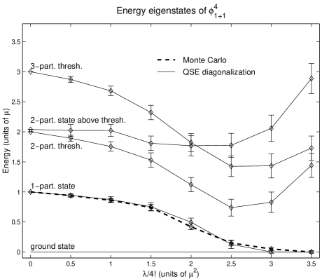
Figure 8: Energy eigenvalues of $\phi_{1+1}^{4}$ as functions of the coupling constant.

The error bars were estimated by repeating the calculation for different values of the auxiliary mass parameter $\mu^{\prime}$.

From prior Monte Carlo calculations we know that the theory has a phase transition at $\frac{\lambda}{4!}\approx 2.5\mu^{2}$ corresponding with spontaneous breaking of the $\phi\rightarrow-\phi$ reflection symmetry.  In the broken phase there are two degenerate ground states and we refer to these as the even and odd vacuum states.  In Figure 8 we see signs of a second order phase transition near $\frac{\lambda}{4!}\approx 2.5\mu^{2}$.  Since we are working in a finite volume the spectrum is discrete, and we can track the energy eigenvalues as functions of the coupling.  Crossing the phase boundary, we see that the vacuum in the symmetric phase becomes the even vacuum in the broken phase while the one-particle state in the symmetric phase becomes the odd vacuum.  The energy difference between the states is also in agreement with a Monte Carlo calculation of the same quantities.  The state marking the two-particle threshold in the symmetric phase becomes the one-particle state above the odd vacuum, while the state at the three-particle threshold becomes the one-particle state above the even vacuum.  These one-particle states should be degenerate in the infinite volume limit.  One rather unusual feature is the behavior of the first two-particle state above threshold in the symmetric phase.  In the symmetric phase this state lies close to the two-particle threshold.  But as we cross the phase boundary the state which was the two-particle threshold is changed into a one-particle state.  Thus our two-particle state is pushed up even further to become a two-particle state above the even vacuum and we see a pronounced level crossing.

We note that while the one-particle mass vanishes near the critical point, the energies of the two-particle and three-particle thresholds reach a minimum but do not come as close to zero energy.  It is known that this model is repulsive in the two-particle scattering channel.  In a large but finite volume the ground state and one-particle states do not feel significant finite volume effects.  The two-particle state at threshold, however, requires that the two asymptotic particles be widely separated.  In our periodic box of length 2$L$ the maximal separation distance is $L$ and we expect an increase in energy with respect to twice the one-particle mass of size $\sim V(L)$, where $V$ is the potential energy between particles.  Likewise a three-particle state will increase in energy an amount $\sim 3V(2L/3)$.  Our results indicate that finite volume effects for the excited states are significant for this value of $L$.

6 Summary

We have proposed a new approach which combines both diagonalization and Monte Carlo within a computational scheme.  The motivation for our approach is to take advantage of the strengths of the two computational methods in their respective domains. We remedy sign and phase oscillation problems by handling the interactions of the most important basis states exactly using diagonalization, and we deal with storage and CPU problems by stochastically sampling the contribution of the remaining states.  We discussed the diagonalization part of the method in this paper.  The goal of diagonalization within our scheme is to find the most important basis vectors of the low energy eigenstates and treat the interactions among them exactly.  We have introduced a new diagonalization method called quasi-sparse eigenvector diagonalization which achieves this goal efficiently and can operate using any basis, either orthogonal or non-orthogonal, and any sparse Hamiltonian, either real, complex, Hermitian, non-Hermitian, finite-dimensional, or infinite-dimensional.  Quasi-sparse eigenvector diagonalization is the only method we know which can address all of these problems.

We considered three examples which tested the performance of the algorithm.  We found the lowest energy eigenstates for a random sparse real symmetric matrix, the lowest eigenstates (sorted according to the real part of the eigenvalue) for a random sparse complex non-Hermitian matrix, and the lowest energy eigenstates for an infinite-dimensional Hamiltonian defined by $1+1$ dimensional $\phi^{4}$ theory in a periodic box.

We regard QSE diagonalization as only a starting point for the Monte Carlo part of the calculation.  Once the most important basis vectors are found and their interactions treated exactly, a technique called stochastic error correction is used to sample the contribution of the remaining basis vectors.  This method is introduced in [40].

Acknowledgments

We thank P. van Baal, H. S. Seung, H. Sompolinsky, and M. Windoloski for useful discussions.

Chapter 5 Introduction to stochastic error correction methods

1 Introduction

In [39] a new approach was proposed for finding the low-energy eigenstates of very large or infinite-dimensional quantum Hamiltonians.  This proposal combines both diagonalization and Monte Carlo methods, each being used to solve a portion of the problem for which the technique is most efficient.  The first part of the proposal is to diagonalize the Hamiltonian restricted to a subspace containing the most important basis vectors for each low energy eigenstate.  This may be accomplished either through variational techniques or an ab initio method such as quasi-sparse eigenvector (QSE) diagonalization.  The second step is to include the contribution of the remaining basis vectors by Monte Carlo sampling.  The use of diagonalization allows one to consider systems with fermion sign oscillations and extract information about wavefunctions and excited states.  The use of Monte Carlo provides tools to handle the exponential increase in the number of basis states for large volume systems.

The first half of this proposal was discussed in [39].  An adaptive diagonalization algorithm known as the quasi-sparse eigenvector method was introduced to find the most important basis vectors for each low energy eigenstate.  This technique is especially valuable when little is known about the low energy states.  It is also the only method available which can handle non-orthogonal bases, non-Hermitian Hamiltonians, infinite dimensional systems, and which can find several low energy states with like quantum numbers simultaneously.  In this paper we discuss the second half of the diagonalization/Monte Carlo scheme.  We introduce several new Monte Carlo techniques which we call stochastic error correction (SEC).  There are two general varieties of stochastic error correction, methods based on a series expansion and those which are not.  The series method starts with an eigenvector of the Hamiltonian restricted to some starting subspace and then includes the contribution of the remaining basis states as terms in an ordered expansion.  The idea is to form a perturbative expansion centered around a good non-perturbative starting point.

As an example of a non-series method we discuss a technique called the stochastic Lanczos method.  This method again starts with eigenvectors of a Hamiltonian submatrix.  Using these as starting vectors, we define Krylov vectors, $\left|j\right\rangle,H\left|j\right\rangle,H^{2}\left|j\right\rangle\cdots$, similar to standard Lanczos diagonalization.  The new ingredient is that matrix elements between Krylov vectors, $\left\langle j^{\prime}\right|H^{n}\left|j\right\rangle,$ are computed using matrix diffusion Monte Carlo.  Since the method does not rely on a series expansion, it has the advantage that the starting vectors need not be close to the exact eigenvectors.

One can generate a large class of stochastic error correction methods based on other non-series algorithms, various ways of resumming the series expansion, or combinations of the two techniques.  In this introductory paper we concentrate on describing the basic principles and implementation of the series and non-series approaches.  We also present three test problems which demonstrate the potential of the new approach for a range of different problems.  In the first example we determine the low energy spectrum of $\phi_{2+1}^{4}$ theory using QSE diagonalization and first order corrections using the series method.  In the second example we find the low energy spectrum of compact $U(1)$ in $2+1$ dimensions using the stochastic Lanczos method.  In the last example we find the ground state of the $2+1$ dimensional Hubbard model using QSE diagonalization and first order series stochastic error correction.  In each case we compare with published results in the literature.  We conclude with a summary and some general comments on the new computational scheme.

2 Series method

Let $\left|i\right\rangle$ be the eigenvectors of a Hamiltonian $H$ restricted to some subspace $S$.  Let $\left|A_{j}\right\rangle$ be the remaining basis vectors in the full space not contained in $S$.  We can represent $H$ as

$$\left[\begin{array}[c]{cccccc}\lambda_{1}&0&\cdots&\left\langle 1\right|H\left|A_{1}\right\rangle&\left\langle 1\right|H\left|A_{2}\right\rangle&\cdots\\ 0&\lambda_{2}&\cdots&\left\langle 2\right|H\left|A_{1}\right\rangle&\left\langle 2\right|H\left|A_{2}\right\rangle&\cdots\\ \vdots&\vdots&\ddots&\vdots&\vdots&\cdots\\ \left\langle A_{1}\right|H\left|1\right\rangle&\left\langle A_{1}\right|H\left|2\right\rangle&\cdots&E\cdot\lambda_{A_{1}}&\left\langle A_{1}\right|H\left|A_{2}\right\rangle&\cdots\\ \left\langle A_{2}\right|H\left|1\right\rangle&\left\langle A_{2}\right|H\left|2\right\rangle&\cdots&\left\langle A_{2}\right|H\left|A_{1}\right\rangle&E\cdot\lambda_{A_{2}}&\cdots\\ \vdots&\vdots&\vdots&\vdots&\vdots&\ddots\end{array}\right].$$ (1)

We have used Dirac’s bra-ket notation to represent the terms of the matrix.  In cases where the basis is non-orthogonal or the Hamiltonian is non-Hermitian, the precise meaning of terms such as $\left\langle A_{1}\right|H\left|1\right\rangle$ is the action of the dual vector to $\left|A_{1}\right\rangle$ upon the vector $H\left|1\right\rangle$.  We have written the diagonal terms for the basis vectors $\left|A_{j}\right\rangle$ with an explicit factor $E$ for reasons to be explained shortly.

Let us assume that $\left|1\right\rangle$ is close to some exact eigenvector of $H$ which we denote as $\left|1_{\text{full}}\right\rangle$.  More concretely we assume that the components of $\left|1_{\text{full}}\right\rangle$ outside $S$ are small enough so that we can expand in inverse powers of the introduced parameter $E.$  In order to simplify the expansion we choose to shift the diagonal entries so that $\lambda_{1}=0.$

The series method of stochastic error correction is based on the $E^{-1}$ expansion,

$$\left|1_{\text{full}}\right\rangle\propto\left[\begin{array}[c]{c}1\\ c_{2}^{\prime}E^{-1}+c_{2}^{\prime\prime}E^{-2}+\cdots\\ \vdots\\ c_{A_{1}}^{\prime}E^{-1}+c_{A_{1}}^{\prime\prime}E^{-2}+\cdots\\ c_{A_{2}}^{\prime}E^{-1}+c_{A_{2}}^{\prime\prime}E^{-2}+\cdots\\ \vdots\end{array}\right],$$ (2)

$$\lambda_{\text{full}}=\lambda_{1}^{\prime}E^{-1}+\lambda_{1}^{\prime\prime}E^{-2}\cdots.$$ (3)

It is convenient to choose the normalization of the eigenvector such that the $\left|1\right\rangle$ component remains 1.  The convergence of the expansion is controlled by the proximity of $\left|1\right\rangle$ to $\left|1_{\text{full}}\right\rangle$.  If $\left|1\right\rangle$ is not at all close to $\left|1_{\text{full}}\right\rangle$ then it will be necessary to use a non-series method such as the stochastic Lanczos method discussed in the next section.

At first order in $E^{-1}$ we find

$$c_{A_{j}}^{\prime}=-\tfrac{\left\langle A_{j}\right|H\left|1\right\rangle}{\lambda_{A_{j}}}$$ (4)

$$\lambda_{1}^{\prime}=-\sum_{j}\tfrac{\left\langle 1\right|H\left|A_{j}\right\rangle\left\langle A_{j}\right|H\left|1\right\rangle}{\lambda_{A_{j}}}$$ (5)

$$c_{j}^{\prime}=\tfrac{1}{\lambda_{j}}\sum_{k}\tfrac{\left\langle j\right|H\left|A_{k}\right\rangle\left\langle A_{k}\right|H\left|1\right\rangle}{\lambda_{A_{k}}}.$$ (6)

At second order the contributions are

$$c_{A_{j}}^{\prime\prime}=\sum_{k\neq j}\tfrac{\left\langle A_{j}\right|H\left|A_{k}\right\rangle\left\langle A_{k}\right|H\left|1\right\rangle}{\lambda_{A_{j}}\lambda_{A_{k}}}-\sum_{l\neq 1}\sum_{k}\tfrac{\left\langle A_{j}\right|H\left|l\right\rangle\left\langle l\right|H\left|A_{k}\right\rangle\left\langle A_{k}\right|H\left|1\right\rangle}{\lambda_{A_{j}}\lambda_{l}\lambda_{A_{k}}}$$ (7)

$$\lambda_{1}^{\prime\prime}=\sum_{j}\sum_{k\neq j}\tfrac{\left\langle 1\right|H\left|A_{j}\right\rangle\left\langle A_{j}\right|H\left|A_{k}\right\rangle\left\langle A_{k}\right|H\left|1\right\rangle}{\lambda_{A_{j}}\lambda_{A_{k}}}-\sum_{j}\sum_{l\neq 1}\sum_{k}\tfrac{\left\langle 1\right|H\left|A_{j}\right\rangle\left\langle A_{j}\right|H\left|l\right\rangle\left\langle l\right|H\left|A_{k}\right\rangle\left\langle A_{k}\right|H\left|1\right\rangle}{\lambda_{A_{j}}\lambda_{l}\lambda_{A_{k}}}$$ (8)

$$c_{m}^{\prime\prime} =-\sum_{j}\sum_{k\neq j}\tfrac{\left\langle m\right|H\left|A_{j}\right\rangle\left\langle A_{j}\right|H\left|A_{k}\right\rangle\left\langle A_{k}\right|H\left|1\right\rangle}{\lambda_{m}\lambda_{A_{j}}\lambda_{A_{k}}}+\sum_{j}\sum_{l\neq 1}\sum_{k}\tfrac{\left\langle m\right|H\left|A_{j}\right\rangle\left\langle A_{j}\right|H\left|l\right\rangle\left\langle l\right|H\left|A_{k}\right\rangle\left\langle A_{k}\right|H\left|1\right\rangle}{\lambda_{m}\lambda_{A_{j}}\lambda_{l}\lambda_{A_{k}}}$$ (9)

$$-\tfrac{1}{\lambda_{m}}\left[\sum_{j}\tfrac{\left\langle 1\right|H\left|A_{j}\right\rangle\left\langle A_{j}\right|H\left|1\right\rangle}{\lambda_{A_{j}}}\right]\tfrac{1}{\lambda_{m}}\left[\sum_{k}\tfrac{\left\langle m\right|H\left|A_{k}\right\rangle\left\langle A_{k}\right|H\left|1\right\rangle}{\lambda_{A_{k}}}\right].$$

These contributions can be calculated by straightforward Monte Carlo sampling.  All that is required is an efficient way of generating random basis vectors $\left|A_{k}\right\rangle$ with known probability rates.  Let $P(A_{\text{trial}})$ denote the probability of selecting $\left|A_{\text{trial}}\right\rangle$ on a given trial.  If for example we are calculating the first order correction to the eigenvalue, then we have

$$\lambda_{1}^{\prime} =-\sum_{j}\tfrac{\left\langle 1\right|H\left|A_{j}\right\rangle\left\langle A_{j}\right|H\left|1\right\rangle}{\lambda_{A_{j}}}$$ (10)

$$=-\lim_{N\rightarrow\infty}\tfrac{1}{N}\sum_{i=1,\cdots,N}\tfrac{\left\langle 1\right|H\left|A_{\text{trial}(i)}\right\rangle\left\langle A_{\text{trial}(i)}\right|H\left|1\right\rangle}{\lambda_{A_{\text{trial}(i)}}P(A_{\text{trial}(i)})}.$$

3 Stochastic Lanczos

We now consider a method called stochastic Lanczos which does not require the starting vectors to be close to exact eigenvectors of $H.$  This is essential if the eigenvectors of $H$ are not quasi-sparse and require extremely large numbers of basis states to represent accurately.

Let $V$ be the full Hilbert space for our system.  As in the previous section let $S$ be the subspace over which we have diagonalized $H$ exactly.  Let $P_{S}$ be the projection operator for $S$ and let $\lambda_{j}$ and $\left|j\right\rangle$ be the eigenvalues and eigenvectors of $H$ restricted to $S$ so that

$$P_{S}HP_{S}\left|j\right\rangle=\lambda_{j}\left|j\right\rangle.$$ (11)

Let $Z$ be an auxiliary subspace, one which contains $S$ but excludes very high-energy states. Let $P_{Z}$ be the projection operator for $Z$.  We will choose $Z$ such that $P_{Z}HP_{Z}$ is bounded above.  Let$\ a$ be a real constant which is greater than the midpoint of the minimum and maximum eigenvalues of $P_{Z}HP_{Z}$.  As $n\rightarrow\infty$ the operator $\left[P_{Z}(H-a)P_{Z}\right]^{n}$ maps any given state in $Z$ to the corresponding lowest-energy eigenvector of $P_{Z}HP_{Z}$ with non-zero overlap.

The stochastic Lanczos method uses the operators $\left[P_{Z}(H-a)P_{Z}\right]^{n}$ to approximate the low-energy eigenvalues and eigenvectors of $P_{Z}HP_{Z}$.  The goal is to diagonalize $H$ in a subspace spanned by vectors

$$\left|d,j\right\rangle=\left[P_{Z}(H-a)P_{Z}\right]^{d}\left|j\right\rangle,$$ (12)

for several values of $d$ and $j$.  This requires calculating $\left\langle d^{\prime},j^{\prime}\right|\left.d,j\right\rangle$ and $\left\langle d^{\prime},j^{\prime}\right|H\left|d,j\right\rangle$.  If our Hamiltonian matrix is Hermitian, both of these terms can be written in the general form

$$\left\langle j^{\prime}\right|\left[P_{Z}(H-a)P_{Z}\right]^{n}\left|j\right\rangle.$$ (13)

Therefore it suffices to determine the matrix

$$A_{n}\equiv P_{S}\left[P_{Z}(H-a)P_{Z}\right]^{n}P_{S}.$$ (14)

For non-orthogonal bases and non-Hermitian Hamiltonians, the only change is that we use vectors

$$\left[P_{Z}(H-a)P_{Z}\right]^{d}\left|j\right\rangle$$ (15)

to generate approximate right eigenvectors of $H$ and vectors in the dual space

$$\left\langle j\right|\left[P_{Z}(H-a)P_{Z}\right]^{d}$$ (16)

to produce approximate left eigenvectors.  Adding and subtracting $P_{S}(H-a)P_{S}$, we can rewrite

$$A_{n}=P_{S}\left[P_{Z}(H-a)P_{Z}-P_{S}(H-a)P_{S}+P_{S}(H-a)P_{S}\right]^{n}P_{S}.$$ (17)

$A_{n}$ can now be evaluated recursively as

$$A_{n+1}=B_{n+1}+\sum_{m=0,\cdots,n}B_{m}(H-a)A_{n-m},$$ (18)

where

$$B_{n}=P_{S}\left[P_{Z}(H-a)P_{Z}-P_{S}(H-a)P_{S}\right]^{n}P_{S}.$$ (19)

The components of $B_{n}$ are computed by matrix diffusion Monte Carlo.  One could also directly evaluate the components of $A_{n}$.  However the calculation for $B_{n}$ eliminates the need to sample the matrix $P_{S}(H-a)P_{S}$, which is already known.  Any general matrix product $M^{(1)}M^{(2)}\cdots M^{(n)}$ is a sum of degree $n$ monomials,

$$\left[M^{(1)}M^{(2)}\cdots M^{(n)}\right]_{jk}=\sum_{i_{1},\cdots i_{n-1}}M_{ji_{1}}^{(1)}M_{i_{1}i_{2}}^{(2)}\cdots M_{i_{n-1}k}^{(n)}.$$ (20)

We can interpret (20) as a sum over paths through the set of basis vectors of $Z,$

$$\left|j\right\rangle\rightarrow\left|i_{1}\right\rangle\rightarrow\cdots\rightarrow\left|i_{n-1}\right\rangle\rightarrow\left|k\right\rangle\text{,}$$ (21)

with an associated weight $M_{ji_{1}}^{(1)}M_{i_{1}i_{2}}^{(2)}\cdots M_{i_{n-1}k}^{(n)}$.  The components of $B_{n}$ are sampled using ensembles of random walkers.  We refer the interested reader to [32] for a review of methods in diffusion Monte Carlo.

We end the section with a discussion of the fermion sign problem.  The sign problem is a general issue for any Monte Carlo calculation.  For a system with sign oscillations the evaluation of a Euclidean-time Green’s function involves sums

$$\sum_{i}x_{i}$$ (22)

with the property that

$$\frac{\sum_{i}x_{i}}{\sum_{i}\left|x_{i}\right|}\sim\exp(-c\cdot V\cdot T),$$ (23)

where $V$ is the volume, $T$ is the Euclidean time, and $c$ is a positive constant.  We will refer to this term as the cancellation ratio.  The exponential dependence on $V$ and $T$ makes computations difficult even for small systems.

The sign problem will affect the calculation of $B_{n}$ in the stochastic Lanczos algorithm and terms in the series method discussed in the previous section.  The effect however is different from the sign problem in typical Monte Carlo Green’s function calculations.  Stochastic error correction is a calculation of eigenvalues and eigenvectors rather than a sampling of the partition function or the time evolution of a given initial state.  Therefore the quantity of interest is not $\exp(-HT)$ but the action of $H$ or $H^{n}$ on approximate eigenvectors of $H$.  Due to homogeneity in $H$ the explicit volume dependence does not appear in the cancellation ratio.  Instead we find

$$\frac{\sum_{i}x_{i}}{\sum_{i}\left|x_{i}\right|}\sim\exp(-k\cdot n),$$ (24)

where $k$ is a positive constant.  The sign problem will return if the starting point of the SEC calculation is very poor and it becomes necessary to use $n$ such that $k\cdot n$ is large.  However in many cases $k\cdot n$ can be kept small even for large $n$ since the most important part of the Hamiltonian, $P_{S}HP_{S},$ is diagonalized exactly.  In short the sign problem is less severe because stochastic error correction uses the result of subspace diagonalization as its starting point.

4 $\phi^{4}$ theory in $2+1$ dimensions

The first example we consider is $\phi^{4}$ theory in $2+1$ dimensions near the $\phi\rightarrow-\phi$ symmetry restoration phase transition.  We will use QSE diagonalization and the series version of stochastic error correction to probe the low energy spectrum of the theory on both sides of the phase transition.

In [42] Magruder demonstrated the existence of a phase transition in $\phi_{2+1}^{4}$ by extending Chang’s duality argument for $\phi_{1+1}^{4}$.  The statement of the main result is as follows.  Consider the two Lagrange densities

$$\mathcal{L}_{+} =\tfrac{1}{2}\partial_{\nu}\phi\partial^{\nu}\phi-\tfrac{1}{2}\mu_{+}^{2}\phi^{2}-\tfrac{g}{4!}\phi^{4}+\tfrac{1}{2}\delta_{\mu_{+}}^{2}\phi^{2}$$ (25)

$$\mathcal{L}_{-} =\tfrac{1}{2}\partial_{\nu}\phi\partial^{\nu}\phi+\tfrac{1}{4}\mu_{-}^{2}\phi^{2}-\tfrac{g}{4!}\phi^{4}+\tfrac{1}{2}\delta_{\mu_{-}}^{2}\phi^{2}.$$ (26)

The counterterm $\delta_{\mu_{+}}^{2}$ is defined so that in the $\mathcal{L}_{+}$ system the $\phi$ self-energy graphs vanish at zero-momentum up to two-loop order.  By shifting the field

$$\phi=\phi^{\prime}+\sqrt{\tfrac{3\mu_{-}^{2}}{g}}$$ (27)

we note that the same counterterm $\delta_{\mu_{-}}^{2}$ (same mass dependence but $\mu_{+}$ replaced by $\mu_{-}$) is also sufficient to renormalize $\mathcal{L}_{-}$.  By equating $\mathcal{L}_{+}$ and $\mathcal{L}_{-}$ we obtain a duality constraint between the two theories.  One feature of this constraint is that the $g\rightarrow\infty$ limit of $\mathcal{L}_{-}$ is mapped to the $g\rightarrow 0$ limit of $\mathcal{L}_{+}$.  Therefore $\mathcal{L}_{-}$, whose reflection symmetry $\phi\rightarrow-\phi$ is broken at small $g$, must eventually reach the symmetric phase for sufficiently large coupling.

The $\mathcal{L}_{-}$ phase transition was studied using quasi-sparse eigenvector diagonalization with stochastic error correction.  Quantities such as the critical coupling, critical exponents, and the low lying energy spectrum were studied and, where possible, compared with Monte Carlo results.  A full discussion methods and results are presented in [62].  We will very briefly summarize some of the results below.

The two spatial dimensions of our system are taken to be a periodic box of size $2L$ by $2L$. We will use the modal field formalism to describe the Hamiltonian for the theory.  In the following we let the vectors $\vec{n}$ represent ordered integer pairs $(n_{x},n_{y})$ such that $\left|n_{x}\right|,\left|n_{y}\right|\leq N_{\max}$.  The parameter $N_{\max}$ corresponds with a momentum cutoff scale of $\Lambda=N_{\max}\pi/L$.  The modal field Hamiltonian has the form

$$H =\sum_{\vec{n}}\left[-\tfrac{1}{2}\tfrac{\partial}{\partial q_{-\vec{n}}}\tfrac{\partial}{\partial q_{\vec{n}}}+\tfrac{1}{2}\left(\tfrac{\vec{n}^{2}\pi^{2}}{L^{2}}-\tfrac{\mu^{2}}{2}\right)-\tfrac{6b}{(2L)^{2}}\tfrac{g}{4!}+\tfrac{48}{(2L)^{4}}\left(\tfrac{g}{4!}\right)^{2}\alpha_{\vec{n}}\right]q_{-\vec{n}}q_{\vec{n}}$$ (28)

$$+\tfrac{1}{(2L)^{2}}\tfrac{g}{4!}\sum_{\vec{n}_{1}+\vec{n}_{2}+\vec{n}_{3}+\vec{n}_{4}=0}q_{\vec{n}_{1}}q_{\vec{n}_{2}}q_{\vec{n}_{3}}q_{\vec{n}_{4}}$$

where

$$b=\sum_{\vec{n}}\tfrac{1}{2\omega_{\vec{n}}},\qquad\omega_{\vec{n}}=\sqrt{\tfrac{\vec{n}^{2}\pi^{2}}{L^{2}}+\mu^{2}},$$ (29)

and

$$\alpha_{\vec{n}}=\sum_{\vec{n}_{1},\vec{n}_{2}}\tfrac{1}{4\omega_{\vec{n}_{1}}\omega_{\vec{n}_{2}}\omega_{\vec{n}-\vec{n}_{1}-\vec{n}_{2}}(\omega_{\vec{n}_{1}}+\omega_{\vec{n}_{2}}+\omega_{\vec{n}-\vec{n}_{1}-\vec{n}_{2}})}.$$ (30)

In Figure 1 we have plotted the lowest energy eigenstates in the rest frame for $N_{\max}=10$ and $L=3\pi$ (in units where $\mu=1$).  This choice of parameters corresponds with $441$ different momentum modes and a momentum cutoff scale of $\Lambda=3.33\mu$.  The states shown in Figure 1

Figure 1: Energy eigenvalues as functions of $\frac{g}{4!}$ as calculated by QSE diagonalization with first-order error corrections.

are the three lowest eigenstates in the even and odd $\phi\rightarrow-\phi$ symmetry sectors, and the energies are measured relative to the ground state energy.  In our calculation QSE diagonalization was used keeping $500$ Fock states, and the stochastic error correction was computed to first-order using the series method.  Error bars shown include statistical error and an estimate of the contribution from higher order corrections.  We see clear evidence of a second-order phase transition near $\frac{g}{4!}=0.9$.  We have labelled the energies of the states according to their physical interpretation in the symmetric phase.  $E_{1}$ is the energy for the one-particle state, $E_{2}(E_{3})$ is for the two(three)-particle threshold, and $E_{2}^{\prime}(E_{3}^{\prime})$ is for the first state above the two(three)-particle threshold.  At finite volume these energies are continuous functions of the coupling $g$.  One feature which was also observed in $\phi_{1+1}^{4}$ [39] is the crossing of energy levels due to the double degeneracy of states in the broken symmetry phase. $\ E_{3}$ is connected to a one-particle state in the broken phase while $E_{2}^{\prime}$ is connected to a two-particle state.  The levels $E_{2}^{\prime}$ and $E_{3}$ therefore cross near the critical point.

Another interesting phenomenon is the appearance of a bound state in the broken symmetry phase.  In both the odd and even symmetry sectors we can measure the ratio of the two-particle to one-particle energies:

0.22.01(4)1.98(4)0.32.01(4)2.05(4)0.41.95(4)1.96(4)0.51.87(4)1.87(4)0.61.86(4)1.82(4)Table 1Table 1fragments 0.2fragments2.01(4)fragments1.98(4)0.3fragments2.01(4)fragments2.05(4)fragments0.4fragments1.95(4)fragments1.96(4)0.5fragments1.87(4)fragments1.87(4)0.6fragments1.86(4)fragments1.82(4)\overset{\text{Table 1}}{\begin{tabular}[c]{|l|l|l|}\hline\cr$\frac{g}{4!}$&$E_{2}^{\prime}/E_{2}$&$E_{3}^{\prime}/E_{3}$\\ \hline\cr$0.2$&$2.01(4)$&$1.98(4)$\\ \hline\cr$0.3$&$2.01(4)$&$2.05(4)$\\ \hline\cr$0.4$&$1.95(4)$&$1.96(4)$\\ \hline\cr$0.5$&$1.87(4)$&$1.87(4)$\\ \hline\cr$0.6$&$1.86(4)$&$1.82(4)$\\ \hline\cr\end{tabular}}

g!4/E2′E2/E3′E3g!4/E2′E2/E3′E3

These results are consistent with the binding energies reported in [7, 8] and [9], which indicate a ratio of $1.83(3)$ near the critical point.

5 Compact U(1) in 2+1 dimensions

Compact U(1) lattice gauge theory in $2+1$ dimensions is a simple but phenomenologically interesting gauge model.  It is asymptotically free and in the usual continuum limit describes massless non-interacting photons.  On the other hand if the continuum limit is reached by rescaling the mass gap to remain constant, one instead finds a confining theory of massive bosons [19].  The Hamiltonian has the form

$$H=-\sum_{l}\tfrac{\partial^{2}}{\partial A_{l}^{2}}-2x\sum_{P}\cos\theta_{P}.$$ (31)

In (31) $A_{l}$ are link gauge fields, $\theta_{P}$ is the sum of the links circuiting a plaquette,

$$\theta_{P}=A_{l_{1}}+A_{l_{2}}-A_{l_{3}}-A_{l_{4}},$$ (32)

and

$$x=e^{-4}a^{-2}$$ (33)

is the strong coupling parameter, which tends to infinity as the lattice spacing $a$ goes to $0$.  We follow the notation of [21] in which an overall constant factor of $\frac{e^{2}}{2}$ multiplying the right-hand side of (31) is suppressed.  The energy levels we measure are therefore in units of $\frac{e^{2}}{2}$.

The diagonalization of lattice gauge Hamiltonians is constrained by the requirements of gauge invariance.  To preserve gauge invariance it is most convenient to use a basis which diagonalizes the electric field part of the Hamiltonian

$$\left[-\sum_{l}\tfrac{\partial^{2}}{\partial A_{l}^{2}}\right]\bigotimes_{l^{\prime}}\left|n_{l^{\prime}}\right\rangle\cdots=\left[\sum_{l}n_{l}^{2}\right]\bigotimes_{l^{\prime}}\left|n_{l^{\prime}}\right\rangle.$$ (34)

As our next example of stochastic error correction we will address the $4\times 4$ lattice system at $x=1$ using this electric field basis.  In [29] it was noted that this poses a challenge to standard diagonalization techniques.  Even on the small $4\times 4$ lattice a surprisingly large number of states, about $10^{7}\sim 10^{8}$, are needed to accurately describe the low energy spectrum at $x=1$.  This problem can be circumvented by modifying the basis states to incorporate more of the physics of the ground state.  For example one can introduce a disordered background of magnetic flux as suggested in [22], and that approach is followed in an ongoing project [37].  However we would like to directly address the problem described in [29] and show how the stochastic Lanczos method handles the proliferation of large numbers of basis states in the original electric field basis.

We will choose our starting subspace $S$ to include all basis states

$$\bigotimes_{l^{\prime}}\left|n_{l^{\prime}}\right\rangle$$ (35)

which satisfy

$$\sum_{l}n_{l}^{2}\leq 8,$$ (36)

and which can be reached from the strong coupling vacuum by at most two transitions via the plaquette operators $\exp(\pm i\theta_{P})$.  We take the auxiliary space $Z$ to be the subspace spanned by basis vectors

$$\sum_{l}n_{l}^{2}\leq L_{\max}^{2}.$$ (37)

Using matrix diffusion Monte Carlo, we diagonalize the subspace formed by the states

$$\left|d,j\right\rangle=\left[P_{Z}(H-a)P_{Z}\right]^{d}\left|j\right\rangle.$$ (38)

$\left|j\right\rangle$ are the eigenvectors of the Hamiltonian restricted to the original subspace $S$.  In our calculations we use $a=L_{\max}^{2}$ and $d=0,1,\cdots 12$ for cutoff values,

$$L_{\max}^{2}=24,28,32.$$ (39)

In Table 2 we show the results for the ground state energy $E_{0}$ for the different cutoff values $L_{\max}^{2}$ and the extrapolated value at $L_{\max}^{2}=\infty$.  The errors shown are estimated statistical errors.  For comparison we show the results of [21] obtained using Green’s function Monte Carlo (GFMC).

E0−7.394(3)−7.430(3)−7.438(3)−7.442(4)−7.4432(5)Table 2Table 2fragments fragmentsE0fragments7.394(3)fragments7.430(3)fragments7.438(3)fragments7.442(4)fragments7.4432(5)\overset{\text{Table 2}}{\begin{tabular}[c]{|l|l|l|l|l|l|}\hline\cr&$L_{\max}^{2}=24$&$L_{\max}^{2}=28$&$L_{\max}^{2}=32$&$L_{\max}^{2}=\infty$&GFMC\\ \hline\cr$E_{0}$&$-7.394(3)$&$-7.430(3)$&$-7.438(3)$&$-7.442(4)$&$-7.4432(5)$\\ \hline\cr\end{tabular}}

=Lmax224=Lmax228=Lmax232=Lmax2∞GFMC=Lmax224=Lmax228=Lmax232=Lmax2∞GFMC

In Table 3 we show the masses for the lightest six particles in the system extrapolated to the limit $L_{\max}^{2}=\infty$.  We have labelled the particles according to their spin $J$ and sign under conjugation $C:A\rightarrow-A.$ We also include results from [21] for the lowest antisymmetric and symmetric glueballs.

|0−⟩3.03(2)3.01(6)|0+⟩4.03(3)4.05(8)|2−⟩6.8(1)|2+⟩6.8(1)|0+⟩7.0(2)|0−⟩7.1(2)Table 3Table 3fragments fragments|0⟩fragments3.03(2)fragments3.01(6)fragments|0⟩fragments4.03(3)fragments4.05(8)fragments|2⟩fragments6.8(1)missing-subexpressionfragments|2⟩fragments6.8(1)missing-subexpressionfragments|0⟩fragments7.0(2)missing-subexpressionfragments|0⟩fragments7.1(2)missing-subexpression\overset{\text{Table 3}}{\begin{tabular}[c]{|l|l|l|}\hline\cr$J^{C}$&Mass&GFMC\\ \hline\cr$\left|0^{-}\right\rangle$&$3.03(2)$&$3.01(6)$\\ \hline\cr$\left|0^{+}\right\rangle$&$4.03(3)$&$4.05(8)$\\ \hline\cr$\left|2^{-}\right\rangle$&$6.8(1)$&\\ \hline\cr$\left|2^{+}\right\rangle$&$6.8(1)$&\\ \hline\cr$\left|0^{+}\right\rangle$&$7.0(2)$&\\ \hline\cr$\left|0^{-}\right\rangle$&$7.1(2)$&\\ \hline\cr\end{tabular}}

JCMassGFMCJCMassGFMC

The results we find appear in agreement with [21].  Unlike most Monte Carlo algorithms, the SEC method is able to find excited states with the same quantum numbers as lower lying states.  This was also evident in the $\phi_{2+1}^{4}$ example where we could track many different states crossing the phase transition.  The reason for this advantage goes back to the design of stochastic error correction as a Monte Carlo improvement of a diagonalization scheme.  For the $U(1)$ example one can reliably find the eigenvalues and eigenvectors for the first twenty or so states in the low energy spectrum.

6 Hubbard Model

The last example we consider is the two-dimensional Hubbard model defined by the Hamiltonian

$$H=-t\sum_{<i,j>;\;\sigma=\uparrow,\downarrow}(c_{i\sigma}^{\dagger}c_{j\sigma}+c_{j\sigma}^{\dagger}c_{i\sigma})+U\sum_{i}(c_{i\uparrow}^{\dagger}c_{i\uparrow}c_{i\downarrow}^{\dagger}c_{i\downarrow}).$$ (40)

The summation $<i,j>$ is over nearest neighbor pairs. $\ c_{i\sigma}^{\dagger}$($c_{i\sigma}$) is the creation(annihilation) operator for a spin $\sigma$ electron at site $i$. $\ t$ is the hopping parameter, and $U$ controls the on-site Coulomb repulsion. The model has attracted considerable attention in recent years due to its possible connection to $d$-wave pairing and stripe correlations in high-$T_{c}$ cuprate superconductors.  In spite of its simple form, the computational difficulties associated with finding the ground state of the model are substantial even for small systems.  Fermion sign problems render Monte Carlo simulations ineffective for $U$ positive and away from half-filling, and the collective effect of very large numbers of basis Fock states make most diagonalization approaches very difficult. A brief overview of the history and literature pertaining to numerical aspects of the Hubbard model can be found in [53].

In terms of momentum space variables, the Hubbard Hamiltonian on an $N\times N$ periodic lattice has the form

$$H =-2t\sum_{p_{x},p_{y}=0,\cdots,N-1}(\cos\tfrac{2\pi p_{x}}{N}+\cos\tfrac{2\pi p_{y}}{N})\left[c_{p_{x},p_{y}}^{\uparrow\dagger}c_{p_{x},p_{y}}^{\uparrow}+c_{p_{x},p_{y},\sigma}^{\downarrow\dagger}c_{p_{x},p_{y}}^{\downarrow}\right]$$ (41)

$$+\tfrac{U}{N^{2}}\sum_{\begin{subarray}{c}p_{x}-q_{x}+r_{x}-s_{x}=0\operatorname{mod}N\\ p_{y}-q_{y}+r_{y}-s_{y}=0\operatorname{mod}N\end{subarray}}c_{p_{x},p_{y}}^{\uparrow\dagger}c_{q_{x,}q_{y}}^{\uparrow}c_{r_{x},r_{y}}^{\downarrow\dagger}c_{s_{x},s_{y}}^{\downarrow}.$$

As a test of our methods, we use QSE diagonalization with stochastic error correction to find the ground state energy of the $4\times 4$ Hubbard model with $5$ electrons per spin.  The corresponding Hilbert space has about $2\cdot 10^{7}$ dimensions.  For the QSE diagonalization we use momentum Fock states which diagonalize the quadratic part of the Hamiltonian.  The Hamiltonian is invariant under the symmetry group generated by reflections about the $x$ and $y$ axes, interchanges between $x$ and $y,$ and interchanges between $\downarrow$ and $\uparrow$.  We find it convenient to work with symmetrized Fock states.  We will compute stochastic error corrections to first order using the series method.

In Table 4 we present results for the ground state energy.  We encountered no trouble with the sign problem, and in fact one can easily see that each term in the first order series expression (5) is negative definite.  The energies are measured relative to the energy of the Fermi sea at $U=0$.  The errors reported are statistical errors associated with the first order SEC calculation.  Where available, we compare with the results presented in [25], which we label as Exact, Projector Quantum Monte-Carlo (PQMC), and Stochastic Diagonalization (SD).  Stochastic diagonalization is a subspace diagonalization technique similar to QSE but one which uses a different method for selecting the subspace and is based on a variational principle [10].  Although the precise number of basis states used in the SD calculations is not listed, we infer from numbers reported for a modified $4\times 4$ Hubbard system that roughly $10^{5}$ states were used.

U=2t1005001000−.4797−.4945−.5006−.50147​(5)−.50181​(3)−.50198​(1)−.50194−.5010−.44(5)U=4t1005001000−1.620−1.748−1.800−1.8113​(4)−1.8242​(3)−1.8302​(1)−1.8309−1.829−1.8(2)U=5t50010002000−2.558−2.651−2.685−2.7073​(4)−2.7208​(2)−2.7231​(1)−2.7245−2.723−2.9(3)Table 4Table 4fragments fragmentsU2t1005001000.4797.4945.5006.501475.501813.501981fragments.50194fragments.5010fragments.44(5)fragmentsU4t10050010001.6201.7481.8001.811341.824231.83021fragments1.8309fragments1.829fragments1.8(2)fragmentsU5t500100020002.5582.6512.6852.707342.720822.72311fragments2.7245fragments2.723fragments2.9(3)\overset{\text{Table 4}}{\begin{tabular}[c]{|l|l|l|l|l|l|l|}\hline\cr Coupling&States&QSE&QSE+SEC&Exact&SD&PQMC\\ \hline\cr$U=2t$&$\begin{array}[c]{c}100\\ 500\\ 1000\end{array}$&$\begin{array}[c]{c}-.4797\\ -.4945\\ -.5006\end{array}$&$\begin{array}[c]{c}-.50147(5)\\ -.50181(3)\\ -.50198(1)\end{array}$&$-.50194$&$-.5010$&$-.44(5)$\\ \hline\cr$U=4t$&$\begin{array}[c]{c}100\\ 500\\ 1000\end{array}$&$\begin{array}[c]{c}-1.620\\ -1.748\\ -1.800\end{array}$&$\begin{array}[c]{c}-1.8113(4)\\ -1.8242(3)\\ -1.8302(1)\end{array}$&$-1.8309$&$-1.829$&$-1.8(2)$\\ \hline\cr$U=5t$&$\begin{array}[c]{c}500\\ 1000\\ 2000\end{array}$&$\begin{array}[c]{c}-2.558\\ -2.651\\ -2.685\end{array}$&$\begin{array}[c]{c}-2.7073(4)\\ -2.7208(2)\\ -2.7231(1)\end{array}$&$-2.7245$&$-2.723$&$-2.9(3)$\\ \hline\cr\end{tabular}}

CouplingStatesQSEQSE+SECExactSDPQMCCouplingStatesQSEQSE+SECExactSDPQMC

Apparently QSE diagonalization with SEC handles the $4\times 4$ system quite well with relatively few states.  Much larger systems are being studied using both higher series corrections and stochastic Lanczos techniques [50].

7 Summary and comments

In this paper we presented two versions of stochastic error correction, the series method and the stochastic Lanczos method.  The series method starts with eigenvectors of the Hamiltonian restricted to some optimized subspace and includes the contribution of the remaining basis states as an ordered expansion.  The stochastic Lanczos method starts with eigenvectors of a Hamiltonian submatrix and constructs matrix elements of Krylov vectors using matrix diffusion Monte Carlo.  This method has the advantage that the starting vectors need not be close to exact eigenvectors.

We presented three different examples which demonstrate the potential of the new approach for strongly coupled scalar, gauge, and fermionic theories.  In the first example we calculated the low energy spectrum of $\phi_{2+1}^{4}$ using the series method, and in the second example we found the spectrum of compact $U(1)$ in $2+1$ dimensions using the stochastic Lanczos method.  In both examples we found agreement with results from the literature.  We also found that unlike typical Monte Carlo results, the SEC method is able to find the eigenvalues and eigenvectors for excited states with the same quantum numbers as lower lying states.  This advantage is due to its design as a Monte Carlo improvement of a diagonalization scheme.  In the last example we found the ground state of the $2+1$ dimensional Hubbard model using QSE diagonalization and first order series stochastic error correction.  In this calculation we encountered no fermion sign problem and found that our methods yielded very accurate results with far less effort than existing techniques. We believe that the methods we have presented hold considerable potential for studying a wide range of non-perturbative quantum systems and answering questions difficult to address using other methods.

Chapter 6 EQSE Diagonalization of the Hubbard Model

1 Introduction

The enhanced quasi-sparse eigenvector (EQSE) method of solving quantum field theory Hamiltonians is the combination of quasi-sparse eigenvector (QSE) method [39] with a stochastic calculation for the contribution of the remaining basis states [40]. The Hubbard model was chosen as a laboratory for testing this method for several reasons. First, we believed the approach could yield results. The basis vectors can be specified in a few words of data and the Hamiltonian is sparse is momentum space. On the other hand, the ground state of the Hubbard model is known for its inclusion of an extraordinary number of Fock states [1] so the model presents a non-trivial challenge to the quasi-sparse approach. Finally, the Hubbard model is thought to be a physically relevant model for superconductivity [1]. While the description of the model is simple, solutions have been difficult and any promising new approach is worthwhile.

We work on a 2-dimensional spatial lattice with the Hubbard Hamiltonian

$$H=-t\sum_{\footnotesize\begin{array}[]{c}\sigma=\uparrow,\downarrow\\ <i,j>\text{nearest}\end{array}}(c_{i\sigma}^{\dagger}c_{j\sigma}+c_{j\sigma}^{\dagger}c_{i\sigma})+U\sum(c_{i\uparrow}^{\dagger}c_{i\uparrow}c_{i\downarrow}^{\dagger}c_{i\downarrow})$$

There are 2 species of electron so there are 4 possible states for each lattice site. Thus the 8x8 Hubbard model has $4^{64}$ dimensions. Even after using particle conservation to partition the space there are more than $10^{32}$ basis vectors. In this large space the Hamiltonian is clearly sparse But the equality of the off-diagonal elements contributes to an extraordinary number of Fock states in the ground.

It is thought that the D-wave correlator $C_{d_{x^{2}-y^{2}}}(r)$ is an important indicator of superconductivity [25].

2 Hamiltonian Momentum Lattice Formulation

After making space periodic we use the Fock states as our basis set. The Hamiltonian conserves momentum which helps limit the number of relevant basis states.

$$H_{\text{kin}}=-2t\sum(\cos\frac{\pi n}{L}+\cos\frac{\pi p}{L})a_{np,\sigma}^{\dagger}a_{np,\sigma}$$

$$V=\frac{U}{4L^{2}}\sum_{\footnotesize\begin{array}[]{c}k-l+m-n=0\\ p-q+r-s=0\end{array}}a_{kp\uparrow}^{\dagger}a_{lq\uparrow}a_{mr\downarrow}^{\dagger}a^{\downarrow}_{ns\downarrow}$$

There is a 16 member symmetry group generated by reflections in the $x$ and $y$ planes, $x\leftrightarrow y$ and$\downarrow\leftrightarrow\uparrow$. For the purpose of finding the ground state, we use only symmetrized basis states.

The first step in the calculation consists of picking a basis set of size $N$ and diagonalizing its submatrix of the Hamiltonian using the Lanczos method [41]. The $\frac{N}{5}$basis vectors which least contribute to the ground are then discarded, replacements are chosen and the Hamiltonian is again diagonalized. When the ground energy $E_{0}$ obtained in this manner converges the QSE step is complete.

The EQSE is a first order correction to this result. We calculate it stochastically. Let $C$ be a set of basis vectors for the complement of the $N$-dimensional subspace. Then, choosing representative basis vectors $v\in C$ with probability $P(v)$ .

$$E=E_{0}+\text{Average}\frac{FO(v)}{P(v)},\qquad\qquad FO(v)=-\frac{\langle 0|H|v\rangle\langle v|H|0\rangle}{\lambda_{v}}$$

where $|0\rangle$ is the ground state of the $N$ dimensional subspace. The expectation is thus

$$E=E_{0}+\sum_{v\in C}P(v)\frac{FO(v)}{P(v)}.$$

3 Results

Results were obtained for the ground state energy, wavefunction and $d$-wave correlator. The computing time was about 2 days on a 350Mhz Pentium II. Where available, we compare with Husslein et al [25] results labeled Exact, Projector Quantum Monte-Carlo (PQMC), and Stochastic Diagonalization (SD) (which uses a different method of choosing the subspace than QSE).

Ground State Energy 4x4 Hubbard Model($\frac{5}{16}$ occupied)
Coupling	States	QSE	EQSE	Exact	SD	PQMC
	50	-.47471	-.50127(5)
U=2	100	-.47967	-.50147(5)	-.50194	-.501	-.49
	500	-.49454	-.50181(3)
	1000	-.50062	-.50198
	50	-1.5707	-1.80635(5)
U=4	100	-1.6203	-1.8113(4)	-1.8309	-1.829	-1.8(2)
	500	-1.7476	-1.8242(3)
	1000	-1.8003	-1.8302
	50	-2.2450	-2.6663(8)
U=5	100	-2.3322	-2.6724(7)	-2.7245	-2.723	-2.9(3)
	500	-2.5578	-2.7073(4)
	1000	-2.6512	-2.7208(2)
	2000	-2.685	-2.7231
	50	-2.963	-3.615
U=6	100	-3.103	-3.635
	1000	-3.452	-3.697
	2000	-3.595	-3.723

Ground Energy 8x8 Hubbard Model($\frac{25}{64}$ occupied)
Coupling	States	QSE	EQSE
	50	-.281	-2.58(2)
	100	-.443	-2.49(2)
U=2	500	-1.221	-2.40(2)
	1000	-1.751	-2.406(8)
	2000	-1.956	-2.423(9)
	4000	-1.958	-2.427
	50	-.811	-9.18(6)
	100	-1.386	-8.48(6)
U=4	500	-3.449	-7.58(5)
	1000	-4.798	-7.59(3)
	2000	-5.374	-7.620(4)
	4000	-5.387	-7.621(5)
	50	-1.222	-13.33(8)
	100	-1.88	-12.33(8)
U=5	500	-4.65	-10.65(6)
	1000	-6.44	-10.65(3)
	2000	-7.225	-10.671(5)
	4000	-7.236	-10.662(8)
	50	-1.6	-18.2
	100	-2.4	-16.6
U=6	500	-5.9	-13.93(8)
	1000	-8.15	-13.78(4)
	2000	-9.110	-13.888(7)
	4000	-9.113	-13.880(8)

The $d_{x^{2}-y^{2}}$ correlator was also obtained using the QSE algorithm. The 4x4 result again matched that of Husslein et al [25]. The EQSE calculation has not been completed and we therefore omit the data.

4 Conclusion

As we can see, the ground state for the 4x4 Hubbard model can be well described with about 1000 symmetrized states and the 50 state results yield remarkable accuracy when the first order correction is included. In the 8x8 case it is clear that even 4000 states are not sufficient to describe the ground state. The precision of the first-order values will be determined with the completion of higher order calculations.

Further advances will come in the refinement of the enhancement technique. Better importance sampling will speed convergence of second and higher orders contributions. Other extensions will be calculation of excited states of the Hamiltonian, correlation functions, binding energies and other quantities of interest.

Chapter 7 Higher order calculations in the Hubbard model

1 Introduction

The last chapter contained an application of the quasi-sparse eigenvector approach to determining the energy of the Hubbard model. The work was done with a Fock state basis. The 4x4 Hubbard model has few enough states that it is possible to directly diagonalize the Hamiltonian and we were able to compare our results with the exact answer.

The accuracy of the results obviously depended on the dimensionality of the exactly solved subspace, $Q$. We summarize here the results for a $U/t$ ratio of $4$, which may be in the physically relevant range for High-Tc superconductivity. A subspace spanned by 50 symmetrized states yielded the ground state energy to within 15%. This slowly declined as we increased the dimensionality. A dimensionality of 1000 was sufficient to within 2%. On the other hand, a first order perturbative calculation (EQSE), when applied to the 50 state space was also sufficient to achieve 1% accuracy and when applied to the 1000 state space the answer was accurate to 4 significant figures.

For the 8x8 Hubbard model the situation was much less clear. While quasi-sparse and first-order corrected results were obtained, their accuracy could not assessed. The EQSE results appear to converge for large initial subspaces. However, a close look shows that the uncorrected quasi-sparse result also appears to converge for $Q$ over about 1200 states. The change from 2000 to 4000 states only lowers the ground energy by about .01 units. But the first order result is more than 2 units lower still. This is evidence of the extreme number of Fock states in the Hubbard ground. Even if there is no further falloff in contribution, one could estimate from this that a quasi-sparse calculation with 400,000 symmetrized basis states in $Q$ would be required to reach the accuracy of the the first order result.

The purpose of this paper is to further explore the ground state energy of the Hubbard model using several approaches including variations of the ordered expansion and the stochastic Lanczos method presented in chapter 6.

2 Calculations

On a 4x4 lattice with 5 occupied sites for both spins, the perturbative ground is given by

$$\begin{array}[]{ccccc}2&.&.&.&.\\ 1&.&\otimes&.&.\\ 0&\otimes&\otimes&\otimes&.\\ -1&.&\otimes&.&.\\ &-1&0&1&2\\ \lx@intercol\hfil\uparrow\text{modes}\hfil\lx@intercol\end{array}\qquad\begin{array}[]{ccccc}2&.&.&.&.\\ 1&.&\otimes&.&.\\ 0&\otimes&\otimes&\otimes&.\\ -1&.&\otimes&.&.\\ &-1&0&1&2\\ \lx@intercol\hfil\downarrow\text{modes}\hfil\lx@intercol\end{array}=|0\rangle$$

A typical excited state is

$$\begin{array}[]{ccccc}2&.&.&.&.\\ 1&\otimes&\otimes&.&.\\ 0&\otimes&\otimes&.&.\\ -1&.&\otimes&.&.\\ &-1&0&1&2\\ \lx@intercol\hfil\uparrow\text{modes}\hfil\lx@intercol\end{array}\qquad\begin{array}[]{ccccc}2&.&.&.&.\\ 1&.&\otimes&.&.\\ 0&\otimes&\otimes&.&.\\ -1&\otimes&\otimes&.&.\\ &-1&0&1&2\\ \lx@intercol\hfil\downarrow\text{modes}\hfil\lx@intercol\end{array}=a_{-11}^{\uparrow\dagger}a_{10}^{\uparrow}a_{-1-1}^{\downarrow\dagger}a_{10}^{\downarrow}|0\rangle$$

We can define a distance function of a state as the number of differences from the perturbative ground. The example above has 2 differences among the $\uparrow$ modes and 2 differences among the $\downarrow$ modes. We say its distance is $(2,2)$. In cases where we are only interested in the greater of the up and down distances we would say the distance is $2$.

When the ground state energy computed in chapter 7 was considered as a function of the number of states, we found that the slope would suddenly drop off at around 1200 states for the 8x8 Hubbard model. For the 4x4 case, the drop in slope occurred at around 30 states. The fillings we have used, $5/16$ in the 4x4 case and $25/64$ in the 8x8 case both have a non-degenerate $U=0$ ground state. On close examination, it became clear that the first states found in the quasi-sparse diagonalization were always distance $(2,2)$. When these states, for which $H$ has non-zero matrix elements with the free ground state, were exhausted, the slope of the energy curve would flatten out.

The calculations presented in this chapter all used the natural cutoff of distance $\leq$ 2 to define $Q$, the base subspace. This simple definition saved time in determining if new states were contained in the base subspace. Further, given this definition of $Q$, a clear relationship between powers of $H$ and distance of a state became clear. $H$ has non-zero matrix elements only between states whose relative distance is less than or equal to $2$. As an example, in a calculation of $H^{4}$ between the base space and itself the first and third intermediate states would be states with maximum distance $4$ and the second intermediate state would have maximum distance $6$.

The first extension of the previous results was inclusion of higher order contributions in the ordered expansion. This was done in two ways. Second order Monte Carlo calculations were attempted using the ordered expansion described in chapter 6. The results were on the same order as the first order results and are not presented here. Higher order calculations in this expansion were difficult because of the many different terms that contribute. Instead, the Brillouin-Wigner degenerate perturbation method was used to calculate higher terms. This approach yielded some interesting results which will be discussed.

The other method of extracting data was to use Monte Carlo to calculate the matrix elements of powers of the Hamiltonian. Once these are known there are several ways they can be used. The stochastic Lanczos method uses these matrix elements to generate a matrix for $H$ in a Krylov subspace generated from the ground of the base subspace. In theory one could diagonalize the Krylov subspace to obtain the eigenvectors and eigenvalues of $H$. The usefulness of this method was limited by the very small determinants of the matrix thus created and the uncertainties of the matrix elements calculated using Monte Carlo.

A more careful choice of subspace, using states generated by higher eigenvectors of $Q$ may solve this problem. Although some work was done in this direction, it is not presented here. Instead, we used the power method to extract the eigenvalue using the same matrix elements for $H$.

3 Brillouin-Wigner perturbation theory

The Brillouin-Wigner perturbation method is described in Appendix A. The general idea is to solve a self-consistent equation for the eigenvalue. For the desired eigenvector $|\psi\rangle$ in $Q$, we find the eigenvalue and components as follows.

$$E\langle i|\psi\rangle =(H_{ij}+A^{(1)}_{ij}+A^{(2)}_{ij}+A^{(3)}_{ij}+\ldots)\langle j|\psi\rangle$$

$$H_{ij} =\langle i|H|j\rangle$$

$$A^{(1)}_{ij} =\sum_{|k\rangle\notin Q}\frac{\langle i|H|k\rangle\langle k|H|i\rangle}{E-\langle k|H|k\rangle}$$

$$A^{(2)}_{ij} =\sum_{\scriptsize\begin{array}[]{c}|k\rangle,|l\rangle\notin Q\\ |k\rangle\neq|l\rangle\end{array}}\frac{\langle i|H|k\rangle\langle k|H|l\rangle\langle l|H|i\rangle}{(E-\langle k|H|k\rangle)(E-\langle l|H|l\rangle)}$$

$$A^{(3)}_{ij} =\sum_{\scriptsize\begin{array}[]{c}|k\rangle,|l\rangle,|m\rangle\notin Q\\ |k\rangle\neq|l\rangle,|l\rangle\neq|m\rangle\end{array}}\frac{\langle i|H|k\rangle\langle k|H|l\rangle\langle l|H|m\rangle\langle m|H|i\rangle}{(E-\langle k|H|k\rangle)(E-\langle l|H|l\rangle)(E-\langle m|H|m\rangle)}$$

etc.

This could be solved by feeding the $n$-th order result for $E$ into the $(n+1)$-th order calculation’s denominators. Alternatively we could keep a running estimate for $E$ as the Monte Carlo proceeds and, at each step, use the current estimate. Instead, we chose to calculate the left hand side $E_{l}$ as a function of the right hand side $E_{r}$. We then take the intersection of the graph of this function and the line $E_{l}=E_{r}$ as the eigenvalue.

Each Monte Carlo trial consists of a trajectory beginning and ending in $Q$. At each step the weight is adjusted by the appropriate probabilities and, outside of $Q$ the appropriate denominator is divided. Figure 1

Figure 1: Brillouin-Wigner calculation for energy as a function of order. gnu6_2 and gnu6_3 have max distance 6. The others have max distance 8.

presents data for the 6x6 Hubbard model with $E_{r}=7$. We would have to run this again with $E_{r}=5$ to draw a curve and find the actual eigenvalue. Two of the runs used a distance cutoff of $6$ and two used a distance cutoff of $8$.

A guiding scheme was used to increase the likelihood that paths return to $Q$ and to prevent them from going beyond the cutoff distance. Were it not for the denominators the guiding would be perfect in the sense that all paths would have an equal contribution to the matrix elements. A better guiding scheme would take account of the diagonal energy and better sample those states with smaller denominators.

The convergence is excellent up to order 4 and is good up to order 6 or 7. After that we consistently find values for the minimum eigenvalue that are much too low. One can account for this by the non-linear process of diagonalizing that is used to find the eigenvalue from the $A_{ij}$ matrix. The distance cutoff $6$ and distance cutoff $8$ results remain close at order 5 and 6. After order 7 the noise in the cutoff=$8$ results becomes dominant.

4 Power method

The power method is very simple in theory. We start with the ground state of $H$ restricted to $Q$, run trajectories with $H-a$ and tabulate the results. If the energy shift, $a$, must be chosen such that $|E_{0}-a|>|E_{j}-a|$ for all other eigenvalues $E_{j}$, then the ratio of successive powers of $H$ will approach the value $(E_{0}-a)$.

It is not surprising that the calculation suffers from a sign problem. The guiding, described in the previous section, results in the contributions of different paths at each order being close to each other in magnitude but of varying sign. Functionally, after around 7 or 8 steps this problem significantly adds to the convergence time.

Several modifications were made to minimize the impact of long paths. The first was that only paths outside of $Q$ were tabulated. By restricting to such “connected” paths we decrease the contribution of long paths. Let $\hat{Q}$ be the projector onto the space $Q$ and $\hat{P}=1-\hat{Q}$. And let $C_{n,ij}$ be the $n$-step matrix element between $i$ and $j$ that we get by restricting to paths outside of $Q$.

$$C_{1}= \hat{Q}H\hat{Q}$$

$$C_{n}= (\hat{Q}H\hat{P})(\hat{P}H\hat{P})^{n-2}(\hat{P}H\hat{Q})$$

$$H^{n}= C_{n}+C_{n-1}H^{1}+\ldots C_{1}H^{n-1}$$

The disadvantage of this approach is that it increases the memory needs.

If an intermediate state $|\psi\rangle\notin Q$ is chosen with known probability we can calculate the contribution of paths that pass through it at the $m$-th step. We multiply the Monte Carlo results for $\langle i|H^{m}|\psi\rangle$ and $\langle\psi|H^{n}|j\rangle$ together to find the contribution to $H^{m+n}_{ij}$. Effectively, this allows the calculation of twice as many steps before the sign problem kicks in. The concern with this approach is that more time is spent on each state at the $m$-th step so the space of possible $m$-th states is not as well sampled. If the contribution to $C_{m+n}$ is a relatively smooth function of the $m$-th state this is not a problem. In practice, this method was only worthwhile for higher order terms.

We present the results for the 8x8 Hubbard model in figure 2.

Figure 2: 8x8 Hubbard model: Ratio of $\langle\psi|H^{n}|\psi\rangle$ over $\langle\psi|H^{n-1}|\psi\rangle$ as a function of $n$. Two trials are shown as well as their best fit curves.

The distance function was limited to a maximum of $8$. We plot the ratio of $H^{n}/H^{n-1}$ for $n=1$ to $11$. The energy shift is set to $30$. Two trials were run. $C_{1}$ through $C_{7}$ were calculated with paths starting in $Q$ and $C_{8}$ through $C_{11}$ used the intermediate state method. As expected, the paths approach a decaying exponential. Using gnuplot to fit points $5$ through $11$ yields an asymptotic value of $-39.74$ for one trial and $-39.75$ for the other. Other choices of points to fit result in small changes in these results. Overall, for a distance cutoff of $8$, the 8x8 Hubbard model yields a ground state energy of $-9.74\pm.05$.

We present results for the 6x6 Hubbard model in figure 3.

Figure 3: 6x6 Hubbard model: Ratio of $\langle\psi|H^{n}|\psi\rangle$ over $\langle\psi|H^{n-1}|\psi\rangle$ as a function of $n$. Two trials with max distance 6 and two trials with max distance 8 are shown as well as their best fit curves.

With a distance cutoff of 6, both curves are on top of each other and yield an energy of -4.887. With a distance cutoff of 8 the answer is -4.94. In these calculations the intermediate state method was not used so the results at $n>7$ show larger errors and are not included in the fit.

5 Conclusions

For the computing power we had available, the 8x8 Hubbard model poses a serious challenge. We have been able to extract a good estimate for the ground state energy in the $\frac{25}{64}$ filled sector. The same techniques may also work for calculating correlators in the ground state. The most powerful approach we have used is the power method but the matrices $C_{n}$ extracted for this method are also available for other methods of analysis such as the modified stochastic Lanczos method alluded to above. While the Brillouin-Wigner method may hold promise for the future, it was less precise for our purposes than the power method. The non-linearity of the inversion step makes it particularly sensitive to noisy data. Improvements in guiding or sampling strategies and filters to allow linear treatment of noisy data may help both the Brillouin-Wigner and power method approaches.

states20004000200040001200E-5.374-5.387-7.620-7.621(5)-9.74(5)8x8 Hubbard model, U=48x8 Hubbard model, U=4fragments states20004000200040001200E-5.374-5.387-7.620-7.621(5)-9.74(5)\overset{\text{8x8 Hubbard model, U=4}}{\begin{tabular}[c]{|l|l|l|l|l|l|}\hline\cr method&\lx@intercol\hfil QSE\hfil\lx@intercol &\lx@intercol\hfil first order correction\hfil\lx@intercol &power method\\ \hline\cr states&2000&4000&2000&4000&1200\\ \hline\cr E&-5.374&-5.387&-7.620&-7.621(5)&-9.74(5)\\ \hline\cr\end{tabular}}

methodQSEfirst order correctionpower methodmethodQSEfirst order correctionpower method

A brief look at the summary of results for the ground energy shows that despite the apparent convergence of the first-order correction, the answer is still far from correct. Computations for distance cutoffs of 6 and 10 will allow a determination of the precision of the power method result presented here.

Another interesting extension will be the calculation of ground state energy for other fillings. Exploring the fillings near the one presented here will allow determination of the energy to add or remove an electron from the lattice.

Chapter 8 Degenerate Perturbation Theory

Let $|1\rangle$, $|2\rangle$ …$|n\rangle$ …be eigenstates of $H_{0}$ with energies $E_{n}$. Assume $E_{1}$ through $E_{m}$ are near each other but are all sufficiently far from $E_{m+1}$, $E_{m+2}$ etc. And let $|\psi\rangle$ be an eigenstate of $(H_{0}+V)$ with eigenvalue $W$ where $W$ is close to the $E_{1}$ through $E_{m}$.

By the eigenvalue equation

$$(H_{0}+V)|\psi\rangle=W|\psi\rangle$$

which if we expand $|\psi\rangle$ in terms of $|n\rangle$ becomes

$$\sum_{n}(H_{0}+V)|n\rangle\langle n|\psi\rangle=W\sum_{n}|n\rangle\langle n|\psi\rangle$$

So, taking a contraction with $\langle i|$ on the left we get

$$E_{i}\langle i|\psi\rangle+\sum_{n}\langle i|V|n\rangle\langle n|\psi\rangle=W\langle i|\psi\rangle$$ (1)

This is just an (infinite dimensional) eigenvalue matrix equation.

$$\left[\begin{array}[]{cccc}E_{1}+\langle 1|V|1\rangle&\langle 1|V|2\rangle&\langle 1|V|3\rangle&...\\ \langle 2|V|1\rangle&E_{2}+\langle 2|V|2\rangle&\langle 2|V|3\rangle&...\\ \langle 3|V|1\rangle&\langle 3|V|2\rangle&E_{3}+\langle 2|V|3\rangle&...\\ \vdots&\vdots&\vdots&\ddots\\ \end{array}\right]\left[\begin{array}[]{c}\langle 1|\psi\rangle\\ \langle 2|\psi\rangle\\ \langle 3|\psi\rangle\\ \vdots\\ \end{array}\right]=W\left[\begin{array}[]{c}\langle 1|\psi\rangle\\ \langle 2|\psi\rangle\\ \langle 3|\psi\rangle\\ \vdots\\ \end{array}\right]$$ (2)

If we temporarily fix the value of $W$ this is just a homogeneous first-order equation in $\langle n|\psi\rangle$. Eqn (2) will only have a solution for special values of $W$, but we can use it to determine $\langle m+1|\psi\rangle$, $\langle m+2|\psi\rangle$, etc. in terms of $\langle 1|\psi\rangle$ through $\langle m|\psi\rangle$.

If we treat $\langle i|\psi\rangle$ as fixed for $i\leq m$ we get the equation

$$\left[S\right]\left[\begin{array}[]{c}\langle m+1|\psi\rangle\\ \langle m+2|\psi\rangle\\ \vdots\\ \end{array}\right]=\left[\begin{array}[]{c}\sum_{i\leq m}\langle m+1|V|i\rangle\langle i|\psi\rangle\\ \sum_{i\leq m}\langle m+2|V|i\rangle\langle i|\psi\rangle\\ \vdots\\ \end{array}\right]$$

where

$$\left[S\right]=\left[\begin{array}[]{ccc}E_{m+1}+\langle m+1|V|m+1\rangle-W&\langle m+1|V|m+2\rangle&...\\ \langle m+2|V|m+1\rangle&E_{m+2}+\langle m+2|V|m+2\rangle-W&...\\ \vdots&\vdots&\ddots\\ \end{array}\right]$$

Since $W$ is not near $E_{n}$ for $n\geq m+1$ and $V$ is small, $[S]$ must have non-zero determinant and be invertible. Since the right hand side is linear in $\langle i|\psi\rangle$ for $i\leq m$ we can ( by multipling by $[S^{-1}]$) express $\langle n|\psi\rangle$ for $n\geq m+1$ as a linear combination of $\langle i|\psi\rangle$ .

For $n\geq m+1$ we therefore write

$$\langle n|\psi\rangle=\sum_{i\leq m}A_{ni}\langle i|\psi\rangle$$

Plugging this into (1) we get

$$(W-E_{n}-\langle n|V|n\rangle)\sum_{i\leq m}A_{ni}\langle i|\psi\rangle=\bigl{(}\sum_{i\leq m}\langle n|V|i\rangle\langle i|\psi\rangle\bigr{)}+\sum_{\begin{array}[]{c}n^{\prime}\neq n\\ n^{\prime}\geq m+1\\ \end{array}}\sum_{i\leq m}\langle n|V|n^{\prime}\rangle A_{n^{\prime}i}\langle i|\psi\rangle$$

which can be solved for $A_{ni}$ by fixing coefficients of $\langle i|\psi\rangle$

$$A_{ni}={1\over W-E_{n}-\langle n|V|n\rangle}\biggl{(}\langle n|V|i\rangle+\sum_{\begin{array}[]{c}n^{\prime}\neq n\\ n^{\prime}\geq m+1\\ \end{array}}\langle n|V|n^{\prime}\rangle A_{n^{\prime}i}\biggr{)}$$ (3)

Although this equation has $A_{n^{\prime}i}$ on the right hand side it could be solved iteratively since the $A_{n^{\prime}i}$ comes with an extra factor of $V$ relative to the $A_{ni}$ on the left hand side. However, remember that $A_{ni}$ is really a function of $W$ so we are not ready to solve it until we find $W$.

Now we are ready to turn to the eigenvalue problem in the $|1\rangle$ through $|m\rangle$ subspace. Once again using eqn (1)

$$W\langle i|\psi\rangle=(E_{i}+\langle i|V|i\rangle)\langle i|\psi\rangle+(\sum_{\begin{array}[]{c}j\neq i\\ j\leq m\\ \end{array}}\langle i|V|j\rangle\langle j|\psi\rangle)+\sum_{\begin{array}[]{c}n\geq m+1\\ \end{array}}\sum_{j\leq m}\langle i|V|n\rangle A_{nj}\langle j|\psi\rangle$$

$$\begin{array}[]{rl}=\biggl{(}&E_{i}+\langle i|V|i\rangle+\sum_{\begin{array}[]{c}n\geq m+1\\ \end{array}}\langle i|V|n\rangle A_{ni}\biggr{)}\langle i|\psi\rangle\\ &+\sum_{\begin{array}[]{c}j\neq i\\ j\leq m\\ \end{array}}\biggl{(}\langle i|V|j\rangle+\sum_{\begin{array}[]{c}n\geq m+1\\ \end{array}}\langle i|V|n\rangle A_{nj}\biggr{)}\langle j|\psi\rangle\end{array}$$ (4)

Equation (4) is an eigenvalue equation, $([M]-W)[\langle i|\psi\rangle]=0$, for $W$ with the $m\times m$ matrix $[M]$ given by

$$M_{ii}=\biggl{(}E_{i}+\langle i|V|i\rangle+\sum_{\begin{array}[]{c}n\geq m+1\\ \end{array}}\langle i|V|n\rangle A_{ni}\biggr{)}$$

and

$$M_{ij}=\biggl{(}\langle i|V|j\rangle+\sum_{\begin{array}[]{c}n\geq m+1\\ \end{array}}\langle i|V|n\rangle A_{nj}\biggr{)}$$

The only problem is that $[M]$ is itself a function of $W$ through $A_{ni}$. Again, however, this can be solved iteratively since the $A_{ni}$ terms all come in with an extra factor of $V$.

So, the general procedure is to solve the eigenvalue equation to first order in $V$ (ignoring all the terms with $A_{ni}$ since $A_{ni}$ itself has order 1) and then to use this $W$ to solve for $A_{ni}$ to first order. (We can ignore the terms with $A_{n^{\prime}i}$ on the right hand side since they are second order in $V$.) Now we can continue by substituting the first order value of $A_{ni}$ into $[M]$ and now calculating $W$ to second order. If we substitute this and the first order values for $A_{n^{\prime}i}$ into (3) we can solve for $A_{ni}$ to second order.

At order $k$ we solve the eigenvalue equation for $W$ using $A_{ni}$ to order $(k-1)$ and then use $W$ to order $k$ and $A_{n^{\prime}i}$ to order $(k-1)$ to solve for $A_{ni}$ to order $k$. Of course, there are $m$ solutions for $W$ at order $k$ and we have to match the solution used for order $(k-1)$. [49]

References

- [1] P. W. Anderson. Science, 235:1196, 1987.
- [2] C. Bender, S. Pinsky, and B. van de Sande. Phys. Rev. D, 48:816, 1993.
- [3] P. Biswas, P. Cain, R. Römer, and M. Schreiber. cond-mat/0001315, 2000.
- [4] N. Bogoliubov and O. Parasiuk. Acta Math., 97:227, 1957.
- [5] B. Borasoy and D. Lee. Phys. Lett. B, 447:98, 1999.
- [6] S. Brodsky, H. Pauli, and S. Pinsky. Phys. Rep., 301:299, 1998.
- [7] M. Caselle, M. Hasenbusch, and P. Provero. Nucl. Phys. B, 556:575, 1999.
- [8] M. Caselle, M. Hasenbusch, and P. Provero. hep-lat/9907018, 1999.
- [9] M. Caselle, M. Hasenbusch, P. Provero, and K. Zarembo. hep-th/0001181, 2000.
- [10] H. de Raedt and M. Frick. Comp. Phys. Rep., 7:1, 199.
- [11] F. del Aguila, A. Culatti, R. Munoz-Tapia, and M. Perez-Victoria. hep-th/9806451, 1998.
- [12] G. dell’Antonio, Y. Frishman, and D. Zwanziger. Phys. Rev. D, 6:988, 1972.
- [13] D. Freedman, K. Johnson, and J. Latorre. Nucl. Phys. B, 371:353, 1992.
- [14] S. Fubini, A. Hanson, and R. Jackiw. Phys. Rev. D, 7:1732, 1973.
- [15] L. Girardello and E. Montaldi. Phys. Lett. B, 57:155, 1975.
- [16] W. Glaser. Nuovo Cimento, 9:990, 1958.
- [17] S. Glazek and K. Wilson. Phys. Rev. D, 48:5863, 1993.
- [18] S. Glazek and K. Wilson. Phys. Rev. D, 49:4214, 1994.
- [19] M. Gopfert and G. Mack. Commun. Math. Phys., 82:545, 1982.
- [20] C. Hagen. Nuovo Cimento, 51B:169, 1967.
- [21] C. Hamer, R. Bursill, and M. Samaras. Nucl. Phys. B, , 2000. hep-lat/0002001.
- [22] D. Heys and D. Stump. Phys. Rev. D, 28:2067, 1983.
- [23] L. Hollenberg. Phys. Rev. D, 47:1640, 1993.
- [24] L. Hollenberg. Phys. Rev. D, 50:2293, 1994.
- [25] T. Husslein, W. Fettes, and I. Morgenstern. Int. J. Mod. Phys. C, Vol. 8 No. 2:397, 1997.
- [26] E. Brooks III and S. Frautschi. Z. Phys. C, 14:27, 1982.
- [27] E. Brooks III and S. Frautschi. Z. Phys. C, 23:263, 1984.
- [28] M. Inui, S. Trugman, and E. Abrahams. Phys. Rev. B, 49:3190, 1994.
- [29] A. Irving, J. Owens, and C. Hamer. Phys. Rev. D, 28:2059, 1983.
- [30] K. Johnson. Ann. Phys., 26:1, 1963.
- [31] B. Klaiber. Helv. Phys. Acta, 37:554, 1964.
- [32] I. Kosztin, B. Faber, and K. Schulten. Amer. J. Phys., 64:633, 1996.
- [33] J. Latorre, C. Manuel, and X. Vilasis-Cardona. Ann. Phys., 231:149, 1994.
- [34] D. Lee. hep-th/0007010, 1997.
- [35] D. Lee. Phys. Lett. B, 439:85, 1998.
- [36] D. Lee. Phys. Lett. B, 444:474, 1998.
- [37] D. Lee and N. Salwen. work in progress.
- [38] D. Lee and N. Salwen. Phys. Lett. B, 460:107, 1999. chapter 2 of this thesis.
- [39] D. Lee, N. Salwen, and Daniel Lee. Phys. Lett. B, 503:223–235, 2001. chapter 5 of this thesis.
- [40] D. Lee, N. Salwen, and M. Windoloski. Phys. Lett. B, 502:329–337, 2001. chapter 6 of this thesis.
- [41] R. Lehoucq, K. Maschhoff, D. Sorensen, and C. Yang. ARPACK: Arnoldi Package, 1997. http://www.caam.rice.edu/software/ARPACK/.
- [42] S. Magruder. Phys. Rev. D, 14:1602, 1976.
- [43] P. Marrero, E. Roura, and D. Lee. Phys. Lett. B, 471:45, 1999.
- [44] A. Mueller and T. Trueman. Phys. Rev. D, 4:1635, 1971.
- [45] N. Nakanishi. Prog. of Theor. Phys., 57:589, 1977.
- [46] M. Perez-Victoria. hep-th/9808071, 1998.
- [47] R. Perry, A. Harindranath, and K. Wilson. Phys. Rev. Lett., 24:2959, 1990.
- [48] S. Pinsky, B. van de Sande, and J. Hiller. Phys. Rev. D, 51:726, 1995.
- [49] H. Salwen. Phys. Rev., 99:1274, 1955.
- [50] N. Salwen. see chapters 7 and 8.
- [51] N. Salwen and D. Lee. Phys. Lett. B, 468:118, 1999. chapter 3 of this thesis.
- [52] N. Salwen and D. Lee. Phys. Rev. D, 62:025006, 2000. chapter 4 of this thesis.
- [53] D. Scalapino and S. White, 2000. cond-mat/0007515.
- [54] O. Schnetz. J. Math. Phys., 38:738, 1997.
- [55] C. Sommerfield. Ann. Phys., 26:1, 1963.
- [56] C. Soukoulis, I. Weman, G. Grest, and E. Economou. Phys. Rev. B, 26:1838, 1982.
- [57] Y. Taguchi, A. Tanaka, and K. Yamamoto. Prog. of Theor. Phys., 52:1042, 1974.
- [58] W. Thirring. Ann. Phys., 3:91, 1958.
- [59] J. Thomassen. Mod. Phys. Lett. A, 14:745, 1999.
- [60] S. White. Phys. Rev. Lett., 69:2863, 1992.
- [61] S. White. Phys. Rev. B, 48:10345, 1993.
- [62] M. Windoloski. PhD thesis, University of Massachusetts, 2000.
- [63] T. Ziman. Phys. Rev. B, 26:7066, 1982.
- [64] W. Zimmerman. Commun. Math. Phys., 11:1, 1969.
- [65] W. Zimmerman. Commun. Math. Phys., 15:208, 1969.