Massless QED₃ with explicit fermions

Abstract

We study dynamical mass generation in QED in $(2+1)$ dimensions using Hamiltonian lattice methods. We use staggered fermions, and perform simulations with explicit dynamical fermions in the chiral limit. We demonstrate that a recently developed method to reduce the fermion sign problem can successfully be applied to this problem. Our results are in agreement with both the strong coupling expansion and with Euclidean lattice simulations.

I Introduction

Quantum electrodynamics in $(2+1)$ dimensions (QED₃) is a theory which shares a number of important features with quantum chromodynamics in $3+1$ dimensions (QCD) such as dynamical mass generation pisa ; Burkitt:1987nx ; Hands:1989mv ; Dagotto ; dcsb ; pennington ; Luo:kk ; Azcoiti ; Hamer:1997bf ; Hands:2002dv and confinement conf . Since QED₃ is super-renormalizable and has fewer degrees of freedom than QCD, it serves as a valuable laboratory in which to test new methods and ideas related to these phenomena. Aside from its role as a testing ground for QCD, however, QED₃ in itself plays an important role in solid state physics and in particular high-$T_{c}$ superconductivity Dorey:1991kp ; Farakos:1997qi . Recently several studies have pursued a new theoretical approach to cuprate superconductors balents ; franz ; superTc in which one describes the phase transition in the reverse direction, starting from the superconducting state. In this picture the antiferromagnetic phase, for example, corresponds to spontaneous chiral symmetry breaking of massless two-flavor QED₃. But there are also several other phases, and the large chiral manifold of degenerate states explains the complexity of the phase diagram.

There are extensive studies using the Dyson–Schwinger equations dcsb suggesting that chiral symmetry in QED₃ is dynamically broken if the number of fermion flavors is smaller than some critical number $N_{c}\sim 3.3$. However, the scale of this symmetry breaking (i.e. the magnitude of the chiral condensate) is extremely small, and there are also studies pennington suggesting that chiral symmetry is broken for all number of fermion flavors. Quenched lattice simulations have shown clear signs of chiral symmetry breaking, with a condensate $\langle\bar{\psi}\psi\rangle\sim 5\times 10^{-3}$ in units of $e^{4}$, the dimensionful coupling constant Hands:1989mv . The situation for dynamical fermions however is not so clear, especially for an odd number of flavors. There have been Euclidean lattice studies in both compact Burkitt:1987nx and non-compact Dagotto formalisms with different numbers of flavors, all suggesting a very small condensate. The most recent Euclidean lattice study of two-flavor non-compact QED₃ suggests an upper bound for the condensate of $\sim 5\times 10^{-5}$ Hands:2002dv , using large lattices.

On the other hand, Hamiltonian lattice studies of QED₃ with one fermion flavor have suggested a rather large value for the chiral condensate. These studies were based on the strong coupling expansion Hamer:1997bf and variational coupled cluster expansion Luo:kk . The obtained condensate was $\sim 0.28$ Hamer:1997bf , significantly larger than both quenched and two-flavor Euclidean lattice results and about two orders of magnitude larger than the Dyson–Schwinger results for one flavor QED₃.

In this paper we study chiral symmetry breaking in one-flavor massless QED₃. To our knowledge our analysis Maris:2002sc represents the first non-perturbative simulation of lattice gauge theory in more than one spatial dimension with explicit fermions. By explicit fermions, we mean that fermions are not integrated out to yield determinants of the Dirac operator. In the simulation presented here, fermion dynamics are sampled explicitly using fermion worldlines in a gauge-field dependent Hamiltonian. From a theoretical point of view, this is an ideal framework in which to address the fermion structure of the ground state wavefunction. From a computational point of view, however, the approach presents profound difficulties such as the fermion sign problem and complex phase fluctuations due to the gauge field, both of which scale exponentially with the volume of the system. Therefore it is not likely that this approach would be possible for QCD in the near future. However, we do find that by employing the recently developed zone method dean02 , we can control sign and phase problems sufficiently to study chiral symmetry breaking in massless QED₃ on relatively small spatial lattices.

In our study, we find that in the strong coupling region, $y<1$, our results agree very well with the strong coupling expansion Hamer:1997bf . However, the agreement between the strong coupling expansion and our simulations breaks down around $y\sim 1$, and for $y>1$ we see a dramatic decrease in the size of the condensate. These results are in agreement with Euclidean lattice simulations using staggered fermions Burkitt:1987nx , suggesting a very small condensate in the continuum limit, $y\to\infty$.

II QED in $(2+1)$ dimensions

QED₃ is a super-renormalizable theory, with a dimensionful coupling: $e^{2}$ has dimensions of mass. This dimensionful parameter plays a role similar to $\Lambda_{\mathrm{QCD}}$ in QCD. In the chiral limit, it also sets the energy scale. We use 4-component spinors, such that the fermion mass term is even under parity. With one massless fermion flavor, the Hamiltonian exhibits a global $U(2)$ “chiral” symmetry. A fermion mass term breaks this symmetry to a $U(1)\times U(1)$ symmetry. The question is: is this chiral symmetry broken dynamically? The order parameter for this symmetry breaking is the chiral condensate.

II.1 Lattice Hamiltonian

We start with the staggered fermion lattice Hamiltonian on an $L_{1}\times L_{2}$ spatial lattice Hamer:1997bf ,

$$H_{\text{physical}} = \frac{g^{2}}{2a}\big{(}W_{E}+W_{B}+W_{F}\big{)}\,,$$ (1)

with

$$W_{E} = \sum_{\vec{r},j}\big{(}E_{j}(\vec{r})\big{)}^{2}\,,$$ (2)

$$W_{B} = -y^{2}\sum_{\vec{r}}\big{(}U_{p}(\vec{r})+U_{p}^{\dagger}(\vec{r})\big{)}\,,$$ (3)

$$W_{F} = -\mu\sum_{\vec{r}}(-1)^{r_{1}+r_{2}}\chi^{\dagger}(\vec{r})\chi(\vec{r})$$ (4)

$${}+y\sum_{\vec{r},j}\eta_{j}(\vec{r})\chi^{\dagger}(\vec{r})U_{j}(\vec{r})\chi(\vec{r}+\hat{\jmath})+\text{h.c.}\,,$$

where $\eta_{1}(\vec{r})=(-1)^{r_{2}+1}$, $\eta_{2}(\vec{r})=1$, $y=1/g^{2}$, and $U_{p}$ is the plaquette operator given by the product of $U_{j}(\vec{r})$’s circuiting the spatial plaquette anchored at $\vec{r}$,

$$U_{p}(\vec{r})=U_{1}(\vec{r})U_{2}(\vec{r}+\hat{1})U_{1}^{\dagger}(\vec{r}+\hat{2})U_{2}^{\dagger}(\vec{r}).$$ (5)

We use a dimensionless mass parameter $\mu=2m/e^{2}$ and a dimensionless coupling constant $g^{2}=e^{2}a,$ where $a$ is the lattice spacing. We also make the Hamiltonian and time dimensionless: the actual simulations are performed with the dimensionless Hamiltonian

$$H := \frac{2a}{g^{2}}H_{\text{physical}}=W_{E}+W_{B}+W_{F}\,,$$ (6)

in combination with the dimensionless time variable

$$t := \frac{g^{2}}{2a}t_{\text{physical}}\,,$$ (7)

instead of the physical Hamiltonian, Eq. (1).

We use the Dirac matrix representation

$$\gamma_{0}=\left[\begin{array}[c]{cc}\sigma_{3}&0\\ 0&-\sigma_{3}\end{array}\right]\;,\;\;\gamma_{1,2}=\left[\begin{array}[c]{cc}i\sigma_{1,2}&0\\ 0&-i\sigma_{1,2}\end{array}\right]\;.$$

Assuming that $L_{1}$ and $L_{2}$ are even, we stagger the fermion components at the four sites of a $2\times 2$ unit cell

$$\chi_{1}(\vec{r}) \sim (2r_{1},2r_{2})$$ (8)

$$\chi_{2}(\vec{r}) \sim (2r_{1}+1,2r_{2})$$ (9)

$$\chi_{3}(\vec{r}) \sim (2r_{1}+1,2r_{2}+1)$$ (10)

$$\chi_{4}(\vec{r}) \sim (2r_{1},2r_{2}+1)\,.$$ (11)

In the continuum limit the staggered fermions correspond to one flavor of a 4-component fermion Hamer:1997bf ; Burden:qb ,

$$\frac{i^{r_{1}+r_{2}}}{2\sqrt{2}a}\left[\begin{array}[c]{cccc}0&-i&0&1\\ 1&0&-i&0\\ -i&0&1&0\\ 0&1&0&-i\end{array}\right]\left[\begin{array}[c]{c}\chi_{1}(\vec{r})\\ \chi_{2}(\vec{r})\\ \chi_{3}(\vec{r})\\ \chi_{4}(\vec{r})\end{array}\right]\rightarrow\left[\begin{array}[c]{c}\psi_{1}(\vec{r})\\ \psi_{2}(\vec{r})\\ \psi_{3}(\vec{r})\\ \psi_{4}(\vec{r})\end{array}\right]\,.$$ (24)

For the states in our physical Hilbert space we choose a basis that is a tensor product of the gauge field and the fermion field degrees of freedom. For each gauge link field let us define the gauge field basis,

$$U_{j}(\vec{r})|X_{j}(\vec{r})\rangle = e^{iX_{j}(\vec{r})}|X_{j}(\vec{r})\rangle\,,$$ (25)

where each $X_{j}$ is a real number in the interval $[0,2\pi)$. We let $|X\rangle$ be the tensor product of states $|X_{j}(\vec{r})\rangle$ at each link,

$$|X\rangle = \bigotimes_{\vec{r},j}|X_{j}(\vec{r})\rangle\,.$$ (26)

Consider the Green’s function

$$G_{X^{\prime},\alpha^{\prime};X,\alpha}(\Delta t) = \Big{(}\langle\alpha^{\prime}|\otimes\langle X^{\prime}|\Big{)}e^{-H\Delta t}\Big{(}|X\rangle\otimes|\alpha\rangle\Big{)}\,,$$

where $|X\rangle\otimes|\alpha\rangle$ and $|X^{\prime}\rangle\otimes|\alpha^{\prime}\rangle$ are two states in our physical Hilbert space, with $|\alpha\rangle$ and $|\alpha^{\prime}\rangle$ general fermion states. If $\Delta t$ is small and $X_{j}(\vec{r})\approx X^{\prime}_{j}(\vec{r})$ for all $\vec{r}$ and $j$, then

$$G_{X^{\prime},\alpha^{\prime};X,\alpha}(\Delta t)$$ (28)

$$\propto \exp\left[-\tfrac{1}{4\Delta t}\sum_{\vec{r},j}\big{(}X_{j}(\vec{r})-X^{\prime}_{j}(\vec{r})\big{)}^{2}-\Delta t\,W_{B}^{X}\right]$$

$${}\times\langle\alpha^{\prime}|\exp\left[-\Delta t\,W_{F}^{X}\right]|\alpha\rangle\,,$$

where

$$W_{B}^{X} = W_{B}\Big{|}_{U_{j}(\vec{r})=e^{iX_{j}(\vec{r})}}\,,$$ (29)

$$W_{F}^{X} = W_{F}\Big{|}_{U_{j}(\vec{r})=e^{iX_{j}(\vec{r})}}\,.$$ (30)

We can evaluate $G_{X_{f},\alpha_{f};X_{i},\alpha_{i}}(t)$ for general initial and final states and arbitrary $t$ by breaking the exponential in Eq. (LABEL:eq:greens) into $N$ equal time steps and inserting a complete set of states at each time step $\Delta t=t/N$. If $\Delta t$ is small, the sum over intermediate states is dominated by consecutive states that are similar, i.e., the $n^{\text{th}}$ time step is dominated by states which satisfy $X^{(n+1)}_{j}\approx X^{(n)}_{j}$ and thus we can use Eq. (28) repeatedly. If we let $X_{i}=X^{(0)}$, $X_{f}=X^{(N)}$, $\alpha_{i}=\alpha^{(0)}$, and $\alpha_{f}=\alpha^{(N)}$, then

$$G_{X_{f},\alpha_{f};X_{i},\alpha_{i}}(t) = {\textstyle\sum\limits_{\begin{subarray}{c}X^{(1)},...,X^{(N-1)}\\ \alpha^{(1)},...,\alpha^{(N-1)}\end{subarray}}}A^{X,\alpha}\;B^{X}$$ (31)

where

$$A^{X,\alpha} = \prod_{n=0}^{N-1}\big{\langle}\alpha^{(n+1)}\big{|}e^{-\tfrac{t}{N}W_{F}^{X^{(n)}}}\big{|}\alpha^{(n)}\big{\rangle}\,,$$ (32)

$$B^{X} = \prod_{n=0}^{N-1}\exp{\left[-\tfrac{N}{4t}\sum_{\vec{r},j}\big{(}X_{j}^{(n+1)}(\vec{r})-X_{j}^{(n)}(\vec{r})\big{)}^{2}\right]}$$ (33)

$$\hphantom{\prod_{n=0}^{N-1}}\times\exp{\left[-\tfrac{t}{N}W_{B}^{X^{(n)}}\right]}\,.$$

In our simulation the gauge field configurations are updated using the Metropolis algorithm. For each new gauge configuration we compute the evolution of the corresponding time-dependent Hamiltonian in the space of fermionic states. The sampling over fermion states is performed using the worldline formalism worldline , which we now briefly discuss.

II.2 Worldlines

At the $n^{\text{th}}$ time step we have an exponential operator of the form

$$S^{(n)} = e^{-\sum_{\vec{r}}\big{(}H_{0}(\vec{r})+H_{1}^{X^{(n)}}(\vec{r})+H_{2}^{X^{(n)}}(\vec{r})\big{)}}\,,$$ (34)

where

$$H_{0}(\vec{r}) = -\tfrac{N\mu(-1)^{r_{1}+r_{2}}}{t}\chi^{\dagger}(\vec{r})\chi(\vec{r})$$ (35)

$$H_{1}^{X^{(n)}}(\vec{r}) = \tfrac{yN\eta_{1}(\vec{r})e^{iX_{1}^{(n)}(\vec{r})}}{t}\chi^{\dagger}(\vec{r})\chi(\vec{r}+\hat{1})+\text{h.c.}$$ (36)

$$H_{2}^{X^{(n)}}(\vec{r}) = \tfrac{yN\eta_{2}(\vec{r})e^{iX_{2}^{(n)}(\vec{r})}}{t}\chi^{\dagger}(\vec{r})\chi(\vec{r}+\hat{2})+\text{h.c.}$$ (37)

In the following we use the shorthand “e” for even and “o” for odd values of $r_{j}$, $j=1,2$. Let us break up $S^{(n)}$ into a product of four terms,

$$S^{(n)} \approx S_{2;\text{o}}^{(n)}S_{2;\text{e}}^{(n)}S_{1;\text{o}}^{(n)}S_{1;\text{e}}^{(n)}\;,$$ (38)

where

$$S_{j;\text{e/o}}^{(n)} = \exp\left[-\sum_{r_{j;\text{e/o}}}\Big{(}\frac{1}{4}H_{0}(\vec{r})+H_{j}^{X^{(n)}}(\vec{r})\Big{)}\right]\,.$$ (39)

Each $S_{j;\text{e/o}}^{(n)}$ is the product of mutually commuting operators which contain the interactions for an adjacent two-site system. With this decomposition of the time evolution operator, one can trace out the worldline of any individual fermion.

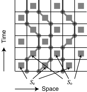
Figure 1: Sample worldline configuration of a system with one spatial dimension.

In Fig. 1 we have drawn the worldlines for a sample worldline configuration. For visual clarity the example we have drawn is a simpler system with only one spatial dimension. We have placed shaded squares where the interactions $S_{j;\text{e/o}}^{(n)}$ occur. In the case when two identical fermions enter the same shaded square we use the convention that the worldlines run parallel and do not cross.

The sum over all worldline configurations is calculated with the help of the loop algorithm loop . At each occupied/unoccupied site, we place an upward/downward pointing arrow as shown in Fig. 2. Due to fermion number conservation, the number of arrows pointing into a shaded square equals the number of arrows pointing out of the square. As a consequence of this conservation law, any valid worldline configuration can be generated from any other worldline configuration by flipping arrows that form closed loops. New Monte Carlo updates are therefore implemented by picking a random closed loop and using the Metropolis condition to determine whether or not to flip the loop.

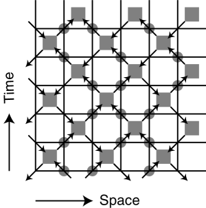
Figure 2: Upward/downward arrows are drawn at each occupied/unoccupied site.

II.3 Measuring the chiral condensate

For $\mu=0$, the staggered lattice formulation reduces the chiral $U(2)$ symmetry to a discrete symmetry generated by a shift of one lattice spacing. To study chiral symmetry breaking on the lattice, we calculate the lattice condensate $\langle\bar{\psi}\psi\rangle$ in the chiral limit as a function of the lattice coupling $y$. The lattice condensate is related to the continuum condensate by the relation

$$y^{2}\langle\bar{\psi}\psi\rangle^{\text{lattice}} = \frac{1}{e^{4}}\langle\bar{\psi}\psi\rangle^{\text{continuum}}\;,$$ (40)

in the limit $y\rightarrow\infty$. From here on $\langle\bar{\psi}\psi\rangle$ will denote $\langle\bar{\psi}\psi\rangle^{\text{lattice}}$. We determine the lattice condensate by computing the limit

$$\lim_{t\rightarrow\infty}\frac{\big{(}\langle\alpha|\otimes\langle F|\big{)}e^{-\frac{Ht}{2}}{\cal O}e^{-\frac{Ht}{2}}\big{(}|F\rangle\otimes|\alpha\rangle\big{)}}{\big{(}\langle\alpha|\otimes\langle F|\big{)}e^{-Ht}\big{(}|F\rangle\otimes|\alpha\rangle\big{)}}\,,$$ (41)

where

$$\cal{O} = -\tfrac{1}{L_{1}L_{2}}\sum_{\vec{r}}(-1)^{r_{1}+r_{2}}\chi^{\dagger}(\vec{r})\chi(\vec{r})\,.$$ (42)

The state $|F\rangle$ is a variational approximation to the gauge field ground state,

$$|F\rangle = \int dX\;F(X)|X\rangle\,,$$ (43)

where

$$F(X)=e^{c\sum_{\vec{r}}\cos\left(X_{1}(\vec{r})+X_{2}(\vec{r}+\hat{1})-X_{1}(\vec{r}+\hat{2})-X_{2}(\vec{r})\right)}\,,$$ (44)

and $c$ is a real parameter we choose to optimize overlap with the true gauge field ground state green's . In our simulations we have used $c=\frac{y}{4}$, which appears to work well for both small and large $y$. The state $|\alpha\rangle$ is the $y=0$ fermion ground state for $\mu>0$, a configuration where even sites are occupied and odd sites are unoccupied. The essential characteristic of the trial state $|F\rangle\otimes|\alpha\rangle$ is that it has non-zero overlap with the physical vacuum.

In Eq. (41), for both numerator and denominator, the initial quantum state is the same as the final state. Any configuration of fermion worldlines can therefore be regarded as a permutation of the initial fermions. Even permutations give a positive contribution while odd permutations come with a minus sign. Numerically, these minus signs give rise to the fermion sign problem. With the worldline formalism we can keep track of these permutations, and we use the recently developed zone method dean02 to manage the sign problem and well as phase oscillations due to the gauge field.

II.4 Zone method

The zone method dean02 consists of introducing a special $n_{1}\times n_{2}$ spatial sub-lattice or zone. See for example Fig. 3.

Figure 3: Illustration of the zone method: an $6\times 8$ spatial lattice with a $3\times 4$ zone. The size of this zone is 17, as characterized by the number of links inside the sub-lattice.

We allow worldline configurations which may permute fermions lying inside this zone, but do not allow configurations that permute any fermions lying outside of the zone. At intermediate time slices though the fermions are still allowed to wander through the entire lattice. In order to control phase oscillations associated with the gauge field, we use a different value of the coupling $y^{\prime}$ and/or fermion mass $\mu^{\prime}$ when the fermions are outside the zone. We obtain physical results by extrapolation to the limit when the zone covers the entire $L_{1}\times L_{2}$ lattice.

As demonstrated in Ref. dean02 , observables should scale linearly in the zone size provided that the zone size is larger than the characteristic “fermion wandering length”. For any finite values of the coupling $y$ and of the time variable $t$, this wandering length is finite, even for massless fermions. Thus one can extrapolate the results from relatively small zones to the entire lattice.

III Numerical results

III.1 Zone Extrapolations

There are different ways to define the size of a zone: by the number of lattice points or by the number of links inside the zone. For large lattices it does not matter which is used. However, for the relatively small lattices we have used so far, it turns out that the best way to characterize the zone size is the number of links inside the zone.

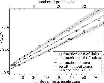
Figure 4: Numerical results for the condensate for different zone sizes within a $6\times 6$ lattice, with fixed values of $y=0.4$, $y^{\prime}=0.1$, $\mu=\mu^{\prime}=0$, $t=1.5$, and $N=10$. The total number of links in the lattice is 72; the total number or points is 36, as is the total area. The straight lines are linear fits to the data.

As an example, we show in Fig. 4 the lattice condensate for different zone sizes as function of the area of the zone, the number of points inside a zone, and the number of links inside a zone. A straight line fit to the condensate as function of the number of links gives a very good fit with a $\chi^{2}$/d.o.f. of 0.6, whereas linear fits using the number of points or the area have a $\chi^{2}$/d.o.f. of 6.1 and 8.5 respectively. Furthermore, the extrapolated result, using the number of links inside a zone, does indeed agree (within error bars) with the exact result.

To further test this method, we calculated the lattice condensate using different parameters $y^{\prime}$ and $\mu^{\prime}$ outside the zone, while keeping the parameters $y$ and $\mu$ inside the zone fixed.

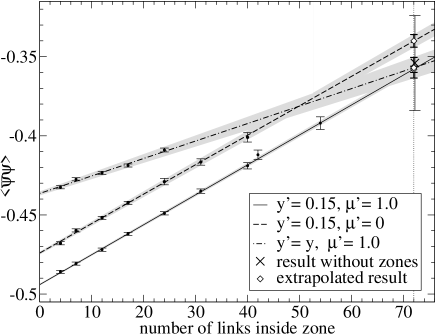
Figure 5: Numerical results for different zone sizes within a $6\times 6$ lattice, for fixed values of $y=0.5$, $\mu=0$, $t=1.5$, and $N=10$. The total number of links in the lattice is 72, where the three linear fits meet (within enlarged error bars).

As can be seen from Fig. 5, the three different sets of data points extrapolate to results within the error bars of the lattice condensate obtained without using the zone extrapolation method. The $\chi^{2}$/d.o.f. of the linear fits are 0.3, 0.7 and 1.2 respectively, indicating that the numerical data are indeed on straight lines.

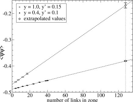
Figure 6: Numerical results for different zone sizes within a $8\times 8$ lattice, for values of $y=0.4$ and $y=1.0$, both with $\mu=0$, $t=1.5$, and $N=10$. The total number of links in the lattice is 128.

Finally, in Fig. 6 we show results on a larger lattice. On an $8\times 8$ lattice the method seems to work quite well, although in this case we cannot compare our result with a simulation on the entire lattice.

III.2 Finite size effects

In order to avoid possible errors due to the zone extrapolation, we checked for finite size effects without the zone method, which limits us to rather small values of $y$ and coarse grids.

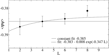
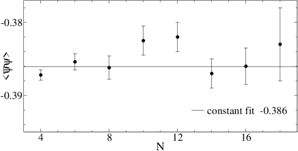
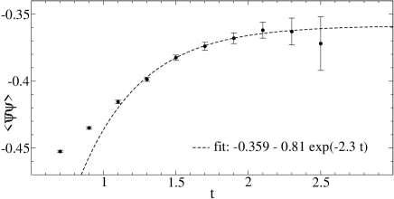
Figure 7: Finite size effects for $y=0.4$, $\mu=0$: the condensate as function of the spatial square lattice of size $L\times L$ for $N=10$ and $t=1.5$ (top), as function of the number of time steps $N$ for $L=4$ and $t=1.5$ (middle), and as function of $t$ for $N=10$ and $L=4$ (bottom).

In Fig. 7 we show for $y=0.4$ the dependence of the chiral condensate on $L$, the spatial lattice size; on $N$, the number of time steps; and on $t$, the dimensionless time variable. We see a slight dependence on $L$, which is actually smaller than our MC error bars. Note that the result for the $8\times 8$ grid was obtained using the zone extrapolation method, where the error bar is the error of the $\chi^{2}$ linear fit only. Within numerical error bars, our results are also independent of the number of time steps, $N$.

The most significant finite-size effect is the dependence on $t$, as can be seen in the bottom panel of Fig. 7. An exponential fit of the type

$$\langle\bar{\psi}{\psi}\rangle(t) = \langle\bar{\psi}{\psi}\rangle(t=\infty)+a_{0}\exp(-a_{1}t)$$ (45)

fits these data quite well for $t>1$. However, for simulations at larger lattices and larger values of $y$ the numerical errors are too large to do a proper finite-$t$ extrapolation using such an exponential fit.

III.3 Summary of main results

In Figs. 8 and 9 we show our results for a range of values of the coupling $y$. Most of the results are obtained on $6\times 6$ spatial lattices with $N=10$ using several different zone sizes. The error bars in Fig. 8 represent the $\chi^{2}$ error of the linear fit from our zone extrapolation. The error bars in Fig. 9 are our best estimate of the combined errors. They are dominated by the $t=\infty$ extrapolation, which is based on three (or more) different values of $t$ where possible. For the largest values of $y$, $y\geq 1.25$, we could only establish upper limits for the condensate, due to the uncertainties in the $t=\infty$ extrapolation.

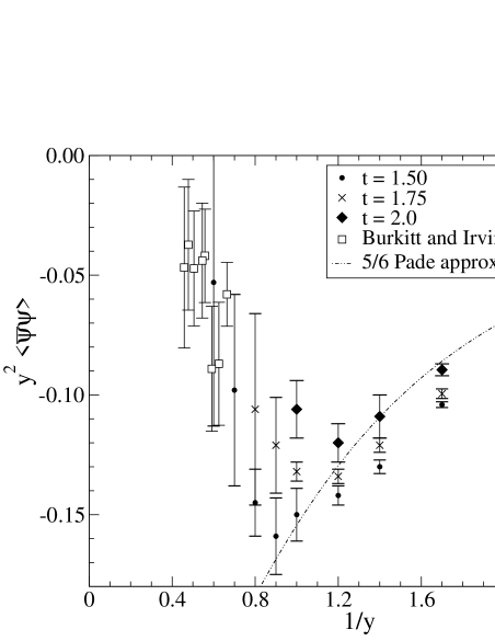
Figure 8: Our results for the lattice condensate as function of $y$ for three different values of $t$ on a $6\times 6$ spatial grid, compared to Euclidean lattice simulations data from Ref. Burkitt:1987nx .

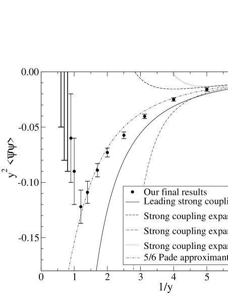
Figure 9: Our results for the lattice condensate as function of $y$, obtained by extrapolating several different zone sizes for a finite value of $t$, compared to the strong coupling expansion Hamer:1997bf .

Our results for the condensate indicate a dramatic change in behavior around $y\sim 1$: for $y<1$ we agree within error bars with the $5/6$ Padé approximant to the strong coupling expansion Hamer:1997bf . For $y\to 0$ our results approach the leading-order behavior in the strong coupling expansion

$$y^{2}\langle\bar{\psi}\psi\rangle^{\text{lattice}} = 0.5\,y^{2}\;,$$ (46)

as expected. However, for $y>1$ we see a dramatic change in the behavior of the condensate, and a deviation from the strong coupling predictions: the value of the condensate decreases rapidly. This strong decrease of the condensate with increasing $y$ for $1<y<2$ is in good agreement with the dynamical Euclidean Monte Carlo simulations by Burkitt and Irving Burkitt:1987nx .

It is not possible to determine at this time whether or not the condensate is small or exactly zero in the continuum limit, $y\rightarrow\infty$. However, it is clear from our simulations that the continuum condensate is significantly smaller than the prediction Hamer:1997bf $y^{2}\langle\bar{\psi}\psi\rangle^{\text{lattice}}\approx 0.284$ based on the strong coupling expansion.

IV Concluding remarks

In this work we studied chiral symmetry breaking in one-flavor massless QED₃, and our analysis represents the first non-perturbative simulation of lattice gauge theory in more than one spatial dimension with explicit fermions. While this approach is likely not practical for QCD in the near future, we were able to use the zone method to control sign and phase problems to study chiral symmetry breaking in massless QED₃.

We were able to resolve one puzzling issue regarding the size of the chiral condensate. Hamiltonian lattice studies had suggested a rather large value for the chiral condensate, whereas lattice simulations and Dyson–Schwinger studies indicated a value for the condensate about two orders of magnitude smaller. In our results we found that for $y>1$ our results agree very well with the strong coupling expansion and the condensate appears to increase as $y$ decreases. However for $1<y<2$ we see a rather dramatic decrease in the condensate as $y$ increases. These results are in agreement with Euclidean lattice simulations using staggered fermions Burkitt:1987nx .

In future studies we would like to study the fermion structure of the ground state wavefunction and to compare and contrast what we see in the simulations with the coupled cluster variational state used in Ref. Luo:kk . We also plan to study the behavior of the chiral condensate as a function of fermion density. We note that studies at finite density in this Hamiltonian formalism are no more difficult computationally than the simulations presented here. Since Euclidean lattice simulations of one-flavor QED₃ at finite density are also afflicted by phase/sign oscillations (which make the computational effort scale exponentially with volume), comparison with explicit fermion simulations in the Hamiltonian framework could provide a valuable numerical check.

- (1) R. D. Pisarski, Phys. Rev. D 29, 2423 (1984).
- (2) A. N. Burkitt and A. C. Irving, Nucl. Phys. B 295, 525 (1988).
- (3) S. Hands and J. B. Kogut, Nucl. Phys. B 335, 455 (1990).
- (4) E. Dagotto, J. B. Kogut and A. Kocic, Phys. Rev. Lett. 62, 1083 (1989); E. Dagotto, A. Kocic and J. B. Kogut, Nucl. Phys. B 334, 279 (1990).
- (5) T. W. Appelquist, M. J. Bowick, D. Karabali and L. C. Wijewardhana, Phys. Rev. D 33, 3704 (1986); T. Appelquist, D. Nash and L. C. Wijewardhana, Phys. Rev. Lett. 60, 2575 (1988); D. Nash, Phys. Rev. Lett. 62, 3024 (1989); P. Maris, Phys. Rev. D 54, 4049 (1996).
- (6) M. R. Pennington and S. P. Webb, Brookhaven preprint BNL-40886; M. R. Pennington and D. Walsh, Phys. Lett. B 253, 246 (1991).
- (7) X. Q. Luo and Q. Z. Chen, Phys. Rev. D 46, 814 (1992).
- (8) V. Azcoiti and X. Q. Luo, Mod. Phys. Lett. A 8, 3635 (1993) [arXiv:hep-lat/9212011]; V. Azcoiti, X. Q. Luo, C. E. Piedrafita, G. Di Carlo, A. F. Grillo and A. Galante, Phys. Lett. B 313, 180 (1993) [arXiv:hep-lat/9305017].
- (9) C. J. Hamer, J. Oitmaa and Z. Weihong, Phys. Rev. D 57, 2523 (1998).
- (10) S. J. Hands, J. B. Kogut and C. G. Strouthos, Nucl. Phys. B 645, 321 (2002) [arXiv:hep-lat/0208030].
- (11) C. J. Burden, J. Praschifka and C. D. Roberts, Phys. Rev. D 46, 2695 (1992); P. Maris, Phys. Rev. D 52, 6087 (1995); G. Grignani, G. W. Semenoff and P. Sodano, Phys. Rev. D 53, 7157 (1996); M. N. Chernodub, E. M. Ilgenfritz and A. Schiller, arXiv:hep-lat/0208013.
- (12) N. Dorey and N. E. Mavromatos, Nucl. Phys. B 386, 614 (1992).
- (13) K. Farakos and N. E. Mavromatos, Mod. Phys. Lett. A 13, 1019 (1998) [arXiv:hep-lat/9707027].
- (14) L. Balents, M. P. A. Fisher and C. Nayak, Phys. Rev. B 60, 1654 (1999).
- (15) M. Franz and Z. Tesanovic, Phys. Rev. Lett. 87, 257003 (2001).
- (16) M. Franz, Z. Tesanovic, and O. Vafek, Phys. Rev. B 65, 180511 (2002); ibid., Phys. Rev. B 66, 054535 (2002); Igor F. Herbut, Phys. Rev. Lett. 88, 047006 (2002); ibid., arXiv:cond-mat/0202491.
- (17) P. Maris and D. Lee, arXiv:hep-lat/0209052.
- (18) Dean Lee, arXiv:cond-mat/0202283; ibid., arXiv:hep-lat/0209047.
- (19) C. J. Burden and C. J. Hamer, Phys. Rev. D 37, 479 (1988).
- (20) J. E. Hirsch, D. J. Scalapino, R. L. Sugar, and R. Blankenbecler, Phys. Rev. Lett. 47, 1628 (1981); ibid., Phys. Rev. B 26, 5033 (1982).
- (21) H. G. Evertz, G. Lana, and M. Marcu, Phys. Rev. Lett. 70, 875 (1993); H. G. Evertz, arXiv:cond-mat/9707221.
- (22) C. J. Hamer, R. J. Bursill, M. Samaras, Phys. Rev. D 62 054511 (2000).