Convergence of Chiral Effective Field Theory

Abstract

We formulate the expansion for the mass of the nucleon as a function of pion mass within chiral perturbation theory using a number of different ultra-violet regularisation schemes; including dimensional regularisation and various finite-ranged regulators. Leading and next-to-leading order non-analytic contributions are included through the standard one-loop Feynman graphs. In addition to the physical nucleon mass, the expansion is constrained by recent, extremely accurate, lattice QCD data obtained with two flavors of dynamical quarks. The extent to which different regulators can describe the chiral expansion is examined, while varying the range of quark mass over which the expansions are matched. Renormalised chiral expansion parameters are recovered from each regularisation prescription and compared. We find that the finite-range regulators produce consistent, model-independent results over a wide range of quark mass sufficient to solve the chiral extrapolation problem in lattice QCD.

I Introduction

The importance of incorporating the chiral non-analytic behavior of hadronic observables in the extrapolation of lattice QCD simulation results has been highlighted in numerous studies over the past few years [1–9]. In an attempt to avoid model dependence, early lattice QCD extrapolations considered simple polynomial functions of the pion mass. However it is now widely accepted that the model-independent, chiral non-analytic behavior predicted by chiral perturbation theory ($\chi$PT) must be incorporated in any quark mass extrapolation function in order to preserve the properties of QCD.

What is more controversial is the manner in which the effective field theory is regulated. Historically, most formulations of $\chi$PT are based on dimensional regularisation and surprisingly other regularisation schemes are often regarded as models. However, the physical predictions of the effective field theory must be regularisation and renormalisation scheme independent, such that other schemes are possible and may provide advantages over the traditional approach. Indeed, Donoghue et al. Donoghue:1998bs have already reported the improved convergence properties of effective field theory formulated with what they call a “long-distance regulator,” such as a dipole or Gaussian form, designed to suppress large three-momentum contributions to the loop integrals of heavy-baryon $\chi$PT.

The origin of the controversy lies in the phenomenological interpretation of the long-distance regulator as a form factor describing the finite size of the meson-cloud source. In this light, it is common to think of the regulator as a model, removing the possibility of systematic improvement through the calculation of higher order terms. However, the interpretation of the regulator as a physical form factor is valid only when the terms analytic in quark mass — the terms involving even powers of $m_{\pi}$ in Eq.(1) below — are either set to zero or determined independent of data by some model of hadron structure. While terms are not constrained by the effective field theory, one can maintain model-independence by including them as parameters fit to data, order by order in the expansion. However there is an obvious corollary of this discussion. To suppress the size of the contributions of the analytic terms, one should consider the use of a phenomenologically motivated regulator. The suppression of the higher-order analytic terms in the corresponding residual expansion that may result from a good choice holds the promise of improved convergence properties in that expansion.

It is extremely important to explore this possibility of improved convergence. At present it is clear that to link full dynamical-fermion lattice QCD simulation results for hadron masses with dimensionally-regulated $\chi$PT, new simulation results are needed in the range from the physical pion mass to 0.1 GeV² Bernard:2002yk ; a daunting task even with the multi-Teraflops resources available over the next five years. Perhaps even more important is the formal issue of the formulation of $SU(3)$-flavor chiral perturbation theory, associated with a strange-quark mass, which likely lies beyond the applicable range of dimensionally-regulated chiral perturbation theory for most baryon observables.

This study will quantitatively compare the chiral expansion of the nucleon mass for six different regularisation schemes, including traditional dimensional regularisation and a variety of long distance regulators. Our focus will be to determine over what range in quark mass (or squared pion mass) all chiral expansions agree at the 1% level. It will become apparent that the long distance regulators do indeed have dramatically improved convergence properties and can imitate the dimensionally regulated chiral expansion over a wider range than the converse. This range will also be reported. Finally, we will discuss the physics, explaining why dimensional regularisation is a poor choice of regulator for effective field theory, in the context of lattice extrapolations. On the other hand, we reach the exciting conclusion that effective field theory formulated with a smooth long-distance regulator provides model-independent chiral expansions agreeing at the 1% level over a range exceeding $0\leq m_{\pi}^{2}\leq 0.8$ GeV². Thus the chiral extrapolation problem has been solved.

II Chiral Effective Field Theory

Chiral perturbation theory ($\chi$PT) is a low-energy effective field theory for QCD. Using this effective field theory, the low-energy properties of hadrons can be expanded about the limit of vanishing momenta and quark mass. In particular, in the context of the extrapolation of lattice data, $\chi$PT provides a functional form applicable as $m_{q}$ approaches zero or, equivalently, $m_{\pi}\to 0$ through the Gell-Mann–Oakes–Renner (GOR) relation $m_{\pi}^{2}\propto m_{q}$ Gell-Mann:1968rz . Goldstone boson loops play an especially important role in the theory as they give rise to non-analytic behaviour as a function of quark mass. The low-order, non-analytic contributions arise from the pole in the Goldstone boson propagator and hence are model-independent Li:1971vr . However, because the analytic variation of hadron properties is not constrained by chiral symmetry, the expansions contain free parameters which must be determined empirically by comparison with data.

Effective field theory then tells us that the formal expansion of the nucleon mass about the SU(2) chiral limit is:

$$M_{N} = a_{0}+a_{2}m_{\pi}^{2}+a_{4}m_{\pi}^{4}$$ (1)

$$+\sigma_{{\rm N}\pi}(m_{\pi},\Lambda)+\sigma_{\Delta\pi}(m_{\pi},\Lambda)+\ldots\,,$$

where $\sigma_{{\rm B}\pi}$ is the self-energy arising from a $B\pi$ loop (with $B$ = $N$ or $\Delta$) and $\Lambda$ is a parameter associated with the regularisation. These $N$ and $\Delta$ loops generate the leading and next-to-leading non-analytic (LNA and NLNA) behaviour, respectively. The expansion has deliberately been written in this form to highlight that the theory is equivalently defined for an arbitrary regulator. This equivalence has been demonstrated by Donoghue et. al. Donoghue:1998bs , where the convergence properties of SU(3) $\chi$PT were improved by implementing a finite-range regulator (FRR), which they term “long-distance regularisation”. More recently this work has been extended to include decuplet baryons Borasoy:2002jv .

The traditional approach within the literature is to use dimensional regularisation to evaluate the self-energy integrals. Under such a scheme the $NN\pi$ contribution simply becomes $\sigma_{{\rm N}\pi}(m_{\pi},\Lambda)\to c_{\rm LNA}m_{\pi}^{3}$ and the analytic terms, $a_{n}m_{\pi}^{n}$ (with $n$ even), undergo an infinite renormalisation. The $\Delta$ contribution produces a logarithm, so that the complete series expansion of the nucleon mass about $m_{\pi}=0$ is:

$$M_{N} = c_{0}+c_{2}m_{\pi}^{2}+c_{4}m_{\pi}^{4}$$ (2)

$$+c_{\rm LNA}m_{\pi}^{3}+c_{\rm NLNA}m_{\pi}^{4}\ln m_{\pi}+\ldots\,,$$

where the $a_{i}$ have been replaced by the renormalised (and finite) parameters $c_{i}$.

As mentioned above, coefficients of low-order non-analytic contributions are known, with Gasser:1988rb ; Lebed:1994yu

$$c_{\rm LNA} = -\frac{3}{32\,\pi\,f_{\pi}^{2}}\,g_{A}^{2}\,,$$

$$c_{\rm NLNA} = \frac{3}{32\,\pi\,f_{\pi}^{2}}\,\frac{32}{25}g_{A}^{2}\,\frac{3}{4\,\pi\,\Delta}\,.$$ (3)

Although strictly one should use values in the chiral limit, we take the experimental numbers with $g_{A}=1.26$, $f_{\pi}=0.093\,{\rm GeV}$, the nucleon–delta mass splitting, $\Delta=0.292\,{\rm GeV}$ and the mass scale associated with the logarithms will be taken to be 1 GeV (i.e. essentially $4\pi f_{\pi}$).

One would expect that it would be possible to reach the physical pion mass from the chiral limit with this expansion truncated beyond $c_{6}m_{\pi}^{6}$. Unfortunately, the convergence of such an expansion seems to break down fairly quickly at higher pion masses. It is also important to realise that Eq. (2) was derived in the limit $m_{\pi}/\Delta\ll 1$. At just twice the physical pion mass this ratio approaches unity. Mathematically the region $m_{\pi}\approx\Delta$ is dominated by a square root branch cut which starts at $m_{\pi}=\Delta$. Using dimensional regularisation this takes the form Banerjee:1996wz :

$$\frac{6g_{A}^{2}}{25\pi^{2}f_{\pi}^{2}}\bigg{[} (\Delta^{2}-m_{\pi}^{2})^{\frac{3}{2}}\ln(\Delta+m_{\pi}-\sqrt{\Delta^{2}-m_{\pi}^{2}})$$ (4)

$$-\frac{\Delta}{2}(2\Delta^{2}-3m_{\pi}^{2})\ln m_{\pi}\bigg{]},$$

for $m_{\pi}<\Delta$, while for $m_{\pi}>\Delta$ the first logarithm becomes an arctangent. Clearly, to access the higher quark masses in the chiral expansion, currently of most relevance to lattice QCD, one requires a more sophisticated expression than that given by Eq. (2).

Even ignoring the $\Delta\pi$ cut for a short time, the formal expansion of the $N\,\rightarrow\,N\,\pi\,\rightarrow\,N$ self-energy integral, $\sigma_{{\rm N}\pi}$, has been shown to have poor convergence properties. Using a sharp, ultra-violet cut-off, Wright showed SVW that the series expansion, truncated at ${\cal O}(m_{\pi}^{4})$, diverged for $m_{\pi}>0.4$ GeV. This already indicated that the series expansion motivated by dimensional regularisation would have a slow rate of convergence.

The main issue of the convergence of this truncated series, Eq. (2), is linked to the formalism in which it is derived from the general form of Eq. (1). The dimensionally regulated approach requires that the pion mass should remain much lighter than every other mass scale involved in the problem. This requires that $m_{\pi}/\Lambda_{\chi{\rm SB}}\ll 1$ and $m_{\pi}/\Delta\ll 1$. An additional scale, mentioned briefly above, is set by the physical extent of the source of the pion field. This scale, which is of order $R_{SOURCE}^{-1}$, corresponds to the transition between the rapid, non-linear variation required by chiral symmetry and the smooth, constituent-quark like mass behaviour observed in lattice simulations at larger quark mass Cloet:2002eg . An alternative to dimensional regularisation would be to regulate Eq. (1) with a finite ultra-violet cut-off (mass parameter $\Lambda$), which physically corresponds to the fact that the source of the meson cloud is an extended structure.

In summary, while the low-energy effective field theory can be very useful in describing the quark mass dependence of hadron properties at very low values of $m_{\pi}$, its utility in the context of lattice QCD appears to have been limited by the tendency in the literature to focus on a single type of regulator (i.e. dimensional regularisation). We now investigate other possible regularisation schemes in order to see whether they are able to ameliorate the problem.

III Constraining the Chiral Expansion

Here we investigate the effective rate of convergence of the chiral expansions obtained using different functional forms for the regulator, together with an analysis of the dimensionally regulated approach. To analyse the merits of various regularisation schemes, at best, we would require exact knowledge of how the nucleon mass varies with quark mass. Having only one value for the experimental nucleon mass we cannot determine the parameters that govern the quark mass dependence of $M_{N}$ without taking some information from alternate sources.

Lattice QCD provides a non-perturbative method for studying the variation of $M_{N}$ with $m_{\pi}$. In principle, this allows one to fix the parameters of the chiral expansion using data obtained in simulations performed at varying quark mass. Lattice simulations of full QCD are restricted to the use of relatively heavy quarks and hence it is not clear, a priori, whether the effective field theory expansion is capable of linking to even the lightest simulated quark mass where $m_{\pi}\sim 500\,{\rm MeV}$. An analysis of each regularisation scheme is necessary to determine the effective range of applicability.

Taking as input the physical nucleon mass and the latest lattice QCD results of the CP-PACS Collaboration AliKhan:2001tx enables us to constrain an expression for $M_{N}$ as a function of the quark mass. The lattice results have been obtained using improved gluon and quark actions on fine, large volume lattices with high statistics. In this work we concentrate on only those results with $m_{\rm sea}=m_{\rm val}$ and the two largest values of $\beta$ (i.e. the finest lattice spacings, $a\sim 0.09$ – $0.13\,{\rm fm}$). This ensures that the results obtained represent accurate estimates of the continuum, infinite-volume theory at the simulated quark masses. The lattice data lies in the intermediate mass region, with $m_{\pi}^{2}$ between $0.3$ and $0.7\,{\rm GeV}^{2}$. One may ask whether the effective field theory has any applicability at this mass scale. The following analysis will answer this question in a model-independent fashion.

In order to remove the bias of choosing any particular regularisation scheme we allow each scheme to serve as a constraint curve for the other methods. In this way we generate six (one for each regularisation) different constraint curves that describe the quark mass dependence of $M_{N}$. The first case corresponds to the truncated power series obtained through the dimensionally regulated (DR) approach, Eq. (2). We work to analytic order $m_{\pi}^{6}$, which is necessary in order to counter the large, non-analytic contribution arising at order $m_{\pi}^{4}\log m_{\pi}$. The second procedure (labeled “BP”) takes a similar form but the branch point obtained from the dimensionally regularised $N\to\Delta\pi$ transition is retained in its full functional form. That is, the logarithm in Eq. (2) is replaced by the full expression, Eq. (4), which ensures the correct non-analytic structure where the logarithm converts to an arctangent above the branch point. We refer to this form as the dimensionally-regulated branch-point (BP) approach. Finally, we use four different functional forms for the finite-ranged, ultra-violet vertex regulator. These are namely the sharp-cutoff (SC), $\theta(\Lambda-k)$; monopole (MON), $\Lambda^{2}/(\Lambda^{2}+k^{2})$; dipole (DIP), $\Lambda^{4}/(\Lambda^{2}+k^{2})^{2}$; and Gaussian (GAU), $\exp(-k^{2}/\Lambda^{2})$. It is commonly assumed in the literature that the functional form chosen for the finite-range regulator will introduce model dependence Becher:1999he and these rather different forms are chosen in order to test this hypothesis.

Since, in the case of finite-range regularisation, we allow the regulator parameter to be tuned to the lattice QCD data points, we do not require an analytic term at order $m_{\pi}^{6}$. The use of a finite-ranged regulator will implicitly include a term of order $m_{\pi}^{6}$, together with a string of higher order terms. Tuning the regulator parameter optimises the efficiency of the one-loop chiral expansion. In particular, it naturally suppresses the large non-analytic contributions which would otherwise dominate at high pion masses. This is in contrast to the dimensional regulated case, where the inclusion of the term in $m_{\pi}^{6}$ is a practical necessity because of the large, non-analytic contribution at order $m_{\pi}^{4}\ln m_{\pi}$.

Fixing the values of the non-analytic contributions to their model-independent values, we have four remaining parameters to be constrained for each of the regularisation schemes. All of the regularisation schemes are constrained simultaneously to fit the physical nucleon mass as well as the lattice QCD data. The resultant curves are displayed in Fig. 1.

Figure 1: Various regularisation schemes providing constraint curves for the variation of $M_{N}$ with pion mass. The short dash curve corresponds to the simple dimensional regularisation scheme (DR) and the long dash curve to the more sophisticated dimensionally regulated approach (BP), which keeps the correct non-analytic structure at the $\Delta\pi$ branch point. The four finite-range regulators (solid curves) are indistinguishable at this scale. Oscillations of the dimensionally regulated schemes (dashed curves) about the solid lines are apparent.

To the naked eye all of the curves are very much in agreement with each other. All of them are able to give an accurate description of the lattice data and match the physical value of $M_{N}$.

Now the question that we pose is: if any one of these curves were presumed to produce an exact description of the mass of the nucleon as a function of $m_{\pi}$, how well could an alternate regularisation scheme match it? All forms have been based on the same, low-energy effective field theory and therefore will be equivalent in the limit $m_{q}\to 0$. Hence, an additional question of more direct practical importance is: over what range can a particular regularisation scheme match an alternate scheme? Within the radius of convergence, physical conclusions must be independent of regularisation and renormalisation.

We show the best fit parameters for our constraint curves, $M(m_{\pi})$, in Table 1.

Regulator	$a_{0}$	$a_{2}$	$a_{4}$	$a_{6}$	$\Lambda$
DR	$0.882$	$3.82$	$6.65$	$-4.24$	–
BP	$0.825$	$4.37$	$9.72$	$-2.77$	–
SC	$1.03$	$1.12$	$-0.292$	–	$0.418$
MON	$1.56$	$0.884$	$-0.204$	–	$0.496$
DIP	$1.20$	$0.972$	$-0.229$	–	$0.785$
GAU	$1.12$	$1.01$	$-0.247$	–	$0.616$

Table 1: Bare fit parameters obtained for the constraint curves, $M(m_{\pi})$. All quantities in appropriate powers of GeV. Regularisation schemes include dimensional regularisation (DR), dimensional regularisation maintaining the correct $\Delta\pi$ branch-point (BP), sharp cut-off (SC), monopole (MON), dipole (DIP) and Gaussian (GAU).

It is worth recalling at this stage that the parameters listed in this table are bare quantities and hence renormalisation scheme dependent. If one is to rigorously compare the parameters of the effective field theory, the self-energy contributions need to be Taylor expanded about $m_{\pi}=0$ in order to yield the renormalisation for each of the coefficients in the quark mass expansion about the chiral limit. We refer to the appendix for the details of this procedure. A comparison of the resulting quark-mass expansion for each of the regularisation schemes is shown in Table 2. The most remarkable feature of Table 2 is the very close agreement between the values of the renormalised coefficients, especially for the finite-range regularisation (FRR) schemes. For example, whereas the variation in $a_{0}$ between all four FRR schemes is 50%, the variation in $c_{0}$ is less than half of one percent. For $a_{2}$ the corresponding figure is 30% compared with 9% variation in $c_{2}$. If one excludes the less physical sharp cut-off (SC) regulator, the monopole, dipole and Gaussian results for $c_{2}$ vary by only 2%. Finally, for $c_{4}$ the agreement is good for the latter three schemes.

The comparison between $a_{4}$ and $c_{4}$ is especially important in order to understand why the FRR schemes are so efficient. Whereas the renormalised coefficients are consistently very large for the three smooth FRR schemes, the bare coefficients of the residual expansion are a factor of 100 smaller! That is, once one incorporates the effect of the finite size of the nucleon by smoothly suppressing pion loops for pion masses above 0.4-0.5 GeV, the residual series expansion has vastly improved convergence properties.

In contrast, in order to fit the nucleon mass data over an extended range of pion mass, the dimensional regularisation schemes require bare expansion coefficients which are much larger, 30 times larger in the case of $a_{4}$. Still these coefficients are not large enough to reach the consistent values of the smooth FRR results reported in Table 2. The failure of this method is amply illustrated by the incorrect behaviour of $M_{N}$ as soon as one applies it even slightly outside the fit region – c.f. the behaviour of DR and BP for $m_{\pi}^{2}$ between 0.8 and 1.0 GeV² shown in Fig. 1.

Regulator	$c_{0}$	$c_{2}$	$c_{4}$
DR	$0.882$	$3.82$	$6.65$
BP	$0.885$	$3.64$	$8.50$
SC	$0.894$	$3.09$	$13.5$
MON	$0.898$	$2.80$	$23.6$
DIP	$0.897$	$2.84$	$22.0$
GAU	$0.897$	$2.87$	$20.7$

Table 2: Renormalised chiral expansion parameters for the constraint curves, $M(m_{\pi})$. All quantities in appropriate powers of GeV. Regularisation schemes include dimensional regularisation (DR), dimensional regularisation maintaining the correct $\Delta\pi$ branch-point (BP), sharp cut-off (SC), monopole (MON), dipole (DIP) and Gaussian (GAU).

IV Comparison of Various Regularisation Schemes

With these given constraint curves, $M(m_{\pi})$, we wish to test how well an alternative regularisation technique can reproduce the same curve. For any well-defined quantum field theory, all physical results should be independent of the regularisation and renormalisation schemes. By doing a one-to-one comparison over different ranges of pion mass we are able to determine the effective convergence range of each scheme.

Figure 2: RMS area between the dimensionally regulated constraint curve and other regularisation schemes, $\chi$, plotted as a function of the curve fitting window $(0,m_{W}^{2})$.

Figure 3: RMS area between the improved dimensionally regulated constraint curve and other regularisation schemes, $\chi$, plotted as a function of the curve fitting window $(0,m_{W}^{2})$.

Figure 4: RMS area between the sharp cut-off regulated constraint curve and other regularisation schemes, $\chi$, plotted as a function of the curve fitting window $(0,m_{W}^{2})$.

Figure 5: RMS area between the monopole regulated constraint curve and other regularisation schemes, $\chi$, plotted as a function of the curve fitting window $(0,m_{W}^{2})$.

Figure 6: RMS area between the dipole regulated constraint curve and other regularisation schemes, $\chi$, plotted as a function of the curve fitting window $(0,m_{W}^{2})$.

Figure 7: RMS area between the Gaussian regulated constraint curve and other regularisation schemes, $\chi$, plotted as a function of the curve fitting window $(0,m_{W}^{2})$.

With one constraint curve, $M(m_{\pi})$, we have five alternate curves, $F(m_{\pi})$, containing free parameters, which may be adjusted to fit this constraint. We fit each particular regularisation scheme to our constraint curve over some window, $m_{\pi}\in(0,m_{W})$. In doing so we define a measure, $\chi$, which describes the root-mean-square area between the curves

$$\chi=\sqrt{\int_{0}^{m_{W}^{2}}dm_{\pi}^{2}\,\left[F(m_{\pi})-M(m_{\pi})\right]^{2}}\,.$$ (5)

In practical calculations the integral over $m_{\pi}^{2}$ is approximated by the Riemann sum by dividing the region into $N$ segments of size $h=m_{W}^{2}/N$,

$$\int_{0}^{m_{W}^{2}}dm_{\pi}^{2}\,f(m_{\pi}^{2})\to h\,\sum_{i=1}^{N}f(ih)\,,$$ (6)

where $h$ is fixed to $0.001\,{\rm GeV}^{2}$. For each upper limit, $m_{W}^{2}$, the measure $\chi$ is minimised in the parameter space of the test function form, $F(m_{\pi})$.

All regularisation prescriptions have precisely the same structure in the limit $m_{\pi}\to 0$. As our test window moves out to larger pion mass the variation of $\chi$ will describe the utility of each expansion. As an indicative scale, with $m_{W}^{2}=0.5\,{\rm GeV}^{2}$ a value of $\chi=700\,{\rm MeV}^{2}$ means that the fit function is, on average, within $1\,{\rm MeV}$ of the constraint curve. Accurate reproduction of the expansion coefficients also serves to test the convergence over a given range.

The variation of $\chi$ as a function of the upper limit of the curve matching window, $m_{W}$, is plotted in Figs. 2 to 7. The first feature that one notices is that, if either dimensionally-regularised scheme is used as the constraint curve, all schemes are able to describe it very well for $m_{\pi}^{2}$ up to 0.4 GeV². On the other hand, we see from Figs. 4 through 7 that neither DR nor BP are able to reproduce the behaviour of the FRR constraint curves beyond about 0.25 GeV². However, all of the FRR schemes are able to reproduce the other FRR schemes over a much wider range – in fact, they reproduce them extremely well over the entire range of pion mass considered (up to 0.8 GeV²). Again, the coefficients in Table 2 help us to understand this observation: it is a simple consequence of the improved convergence properties of the residual series expansion once any reasonable FRR scheme is implemented.

V Chiral Coefficients

We are concerned with the chiral expansion properties about the limit of vanishing quark mass. It is important to test how well the low-energy expansion parameters are reproduced as the curve-matching window is increased. Firstly, we take the dimensionally regularised curve as our constraint — i.e., we assume this is the most accurate description of the real world. We show in Fig. 8 the renormalised expansion parameters, $c_{0}$, of the other regulators constrained to the BP curve, as a function of the curve-fitting window. Figure 9 shows a similar plot for the case where the dipole regulator is taken as the constraint curve.

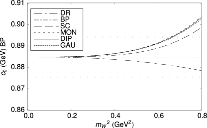
Figure 8: Recovered $c_{0}$ from various regularisation schemes constrained to the dimensionally regularised (BP) curve. $c_{0}$ is plotted as a function of the curve-fitting window $(0,m_{W}^{2})$. The dashed horizontal line indicates the maximum deviation of $c_{0}$ to within 1% of the physical nucleon mass.

Figure 9: Recovered $c_{0}$ from various regularisation schemes constrained to the dipole regularised curve. $c_{0}$ is plotted as a function of the curve-fitting window $(0,m_{W}^{2})$. The dashed horizontal line indicates the maximum deviation of $c_{0}$ to within 1% of the physical nucleon mass.

It is clear from Fig. 8 that, whatever scheme is used to extract $c_{0}$ from the BP constraint curve, it is determined with an accuracy better than 1% as long as the fitting window is smaller than 0.7 GeV². We define our 1% cut such that the contribution to the physical nucleon mass is less than 1% (e.g. in the case of $c_{2}$, this requires that the error in the quantity $c_{2}m_{\pi}^{2}/M_{N}<1\%$ at the physical point).

Conversely, Fig. 9 shows that the dimensional regularisation schemes fail to yield the correct value of $c_{0}$ at the 1% level once the fitting window to the dipole constraint curve extends beyond 0.5 GeV². Yet all the FRR schemes are accurate at a level better than half a percent, whatever window is chosen — with the three smooth schemes accurate to 0.1%.

A similar story applies to the coefficient $c_{2}$, shown in Figs. 10 and 11. All methods yield the correct value of $c_{2}$ based on the BP constraint curve within 1% out to a fit window of 0.7 GeV². The breakdown at this scale should come as little surprise, since the highest lattice data point used to constrain the BP curve lies at around 0.7 GeV².

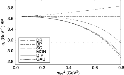
Figure 10: Recovered $c_{2}$ from various regularisation schemes constrained to the dimensionally regularised (BP) curve. $c_{2}$ is plotted as a function of the curve-fitting window $(0,m_{W}^{2})$. The dashed horizontal line indicates the maximum deviation $c_{2}$ can take such that the error in the quantity $c_{2}m_{\pi}^{2}$ is less than 1% of the physical nucleon mass at the physical pion mass.

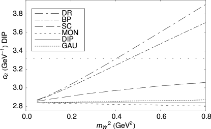
Figure 11: Recovered $c_{2}$ from various regularisation schemes constrained to the dipole regularised curve. $c_{2}$ is plotted as a function of the curve-fitting window $(0,m_{W}^{2})$. The dashed horizontal line is as described in Fig. 10.

When matching to the dipole constraint (Fig. 11), the dimensionally regularised cases break down much earlier, at around 0.4 GeV². All three smooth FRR schemes reproduce this coefficient over the entire range to similar accuracy as found for $c_{0}$.

As we commented in Section III, consistent results are found for the renormalised coefficients $c_{4}$ over the entire fit range $0\leq m_{\pi}^{2}\leq 0.8\,{\rm GeV}^{2}$, provided a smooth finite-range regulator is used to regulate the effective field theory. $c_{4}$ is compromised in the dimensionally-regulated schemes as it attempts to simulate higher-order terms absent in the truncated expansion.

It is clear from these exercises that one cannot hope to use a series expansion based upon dimensional regularisation to analyse data over a window wider than 0.4 GeV². That means one would need to have sufficient, accurate lattice QCD data in this mass region to fix four fitting parameters before one could hope to trust the chiral coefficients so obtained. Within this region, it would also be necessary to have data very near the physical pion mass. This is certainly beyond the likely computational capacity of current collaborations in the next 5-10 years. On the other hand, it is apparent that by using the improved convergence properties of the FRR schemes one can use lattice data in the region up to 0.8 GeV² or greater. This is a regime where we already have impressive data from CP-PACS AliKhan:2001tx and MILC Bernard:2001av . In particular, the FRR approach offers the ability to extract reliable fits where the low-mass region is excluded from the available data. The consideration of this practical application to the extrapolation of lattice data will be discussed further below.

Indeed, these results suggest that given data from the next generation of (10 Teraflops) lattice QCD machines currently under construction, the FRR schemes should allow us to extract $c_{0}$ and $c_{2}$, independent of any model, at the 1% level and $c_{4}$ at the level of a few percent.

VI Discussion and Conclusions

We have observed that all the regularisation schemes produce consistent results for $c_{0}$ and $c_{2}$, with an accuracy sufficient to predict the nucleon mass at the 1% level, provided the expansion is limited to pion masses within the range $0\leq m_{\pi}^{2}\leq 0.4\ {\rm GeV}^{2}$. The curves are very similar with an RMS area between pairs of curves less than 0.001 GeV².

However, it is the dimensionally-regulated curves that are unable to accurately reproduce the results of the finite-range regulated curves beyond the range $0\leq m_{\pi}^{2}\leq 0.4\ {\rm GeV}^{2}$. As contributions from higher order terms not included in the truncated dimensionally-regulated expansion become important, the coefficients of the existing terms move away from their correct values in order to compensate for missing terms.

On the contrary, the finite-range regulated curves are able to reproduce the predictions of dimensional regularisation at the 1% level over a wider range approaching $0\leq m_{\pi}^{2}\leq 0.7\ {\rm GeV}^{2}$. This enhanced range of the finite-range regulated curves is largely a result of the flexibility afforded by the presence of a separate regulation scale, $\Lambda$, which may be adjusted while preserving the excellent convergence properties of the finite-range regulated effective field theory. Hence, one can conclude that the applicable range of finite-range regulated effective field theory in which model independent conclusions may be drawn is $0\leq m_{\pi}^{2}\leq 0.7\ {\rm GeV}^{2}$. This range is sufficient to solve the problem of formulating $SU(3)$-flavor chiral perturbation theory where the strange quark gives rise to a pseudoscalar kaon mass of 0.5 GeV.

However, it is the predictions of dimensional regularisation that prevent this range in pion mass from being larger. Indeed the predictions of each of the smooth finite-range regulated formulations agree at an extraordinarily precise level over the entire range of pion mass considered, $0\leq m_{\pi}^{2}\leq 0.8\ {\rm GeV}^{2}$. This suggests that the more restricted regimes discussed above are associated with a fault in the choice of dimensional regularisation as a regulator for effective field theory in this context.

It is easy to see why this may be. In dimensionally-regularised $\chi$PT, the mass of the pseudoscalar governs the scale of physics contributing to the loop integrals of $\chi$PT. As the pseudoscalar mass increases, the dimensionally-regularised results become dominated by short distance physics; precisely the regime where effective field theory fails because of the internal structure of the hadrons represented by the effective fields. Ignoring this physics by using point-like couplings leads to a badly divergent series expansion at higher order which, in turn, makes the method unsuitable for the lattice extrapolation problem in the foreseeable future.

Fortunately this incorrect short-distance physics, included in dimensionally-regulated loop integrals, can be removed by a more appropriate choice of regulator and a corresponding shift of the parameters of the chiral Lagrangian. In the region where these expansions both converge their predictions must agree as long as the series are not truncated too soon. In a truncated expansion, these incorrect contributions are not removed. In dimensionally-regularised $\chi$PT they become large for increasing $m_{\pi}$, introducing a significant model dependence in the truncated chiral expansion and giving rise to the catastrophic failure already apparent in Fig. 1 for $m_{\pi}^{2}>0.8\ {\rm GeV}^{2}$. Convergence of the dimensionally-regulated expansion is slow as large errors, associated with short-distance physics in loop integrals (not suppressed in dimensionally-regulated $\chi$PT), must be removed by equally large analytic terms.

The enhanced pion-mass range of the finite-range regulated curves is a consequence of the effective resummation of the chiral expansion that arises via the regulator. For example, a Taylor series expansion of the dipole-regulated result for the $N\to N\pi$ self energy of Eq. (19) in the Appendix reveals not only the standard LNA $m_{\pi}^{3}$ contribution, but also new non-analytic contributions proportional to $m_{\pi}^{5}$ and higher powers. As shown by Birse and McGovern, the coefficient of the $m_{\pi}^{5}$ term is related to the Goldberger-Treiman (GT) discrepancy McGovern:1998tm . The coefficients of these new terms involve the dipole regulator parameter $\Lambda$ which can be optimally constrained in the fitting procedure to reproduce the correct non-analytic structure displayed in the data. (Indeed, the sign and magnitude of the coefficient of $m_{\pi}^{5}$ that we find agrees with the value found by Birse and McGovern – although the latter has relatively large errors.) Such terms can only arise at higher order in the dimensionally-regulated expansion as there is no effective re-summation of the series.

It is interesting to note that the appearance of higher-order non-analytic structure, such as the $m_{\pi}^{5}$ term discussed above, does not occur for the special case of the sharp cut-off regulator. An expansion of the arctangent in Eq. (17) provides a constant followed by odd powers of $m_{\pi}$ such that when multiplied by $m_{\pi}^{3}$ only analytic terms appear. This unfortunate feature of the sharp-cutoff regulator explains why it lies between dimensional-regularisation and the smooth finite-range regulated results. While analytic terms can be effectively re-summed, the sharp-cutoff regulator suffers the same restrictions as dimensional regularisation, in that higher-order non-analytic behavior is not effectively re-summed.

The precise agreement between the smooth finite-range regulated results over the entire pion-mass range considered, $0\leq m_{\pi}^{2}\leq 0.8\ {\rm GeV}^{2}$, confirms that the shape of the regulator is irrelevant provided that the regulator parameter is optimised by the fit to the data. An optimal regulator (perhaps guided by phenomenology) effectively re-sums the chiral expansion, encapsulating the essential physics in the first few terms of the expansion. The approach is systematically improved by simply going to higher order in the chiral expansion, introducing additional analytic terms as appropriate to maintain model independence.

It is often argued that dimensionally regularisation works well in the meson sector. However, we know of no reason that the findings discussed here for the baryon sector should not apply equally well there. Improved convergence of finite-range regulated $\chi$PT for meson properties will provide access to a wide range of quark masses and precision determinations of the low-energy constants.

As discussed in the introduction it of great interest how to apply the features of effective field theory to the extrapolation of lattice QCD results. If one wishes to extract the low-energy constants from currently accessible lattice simulations, it is necessary that any such prescription is not sensitive to the choice of regularisation or renormalisation. Here we describe how the FRR schemes achieve this result.

With current lattice data typically restricted to $m_{\pi}^{2}>0.3\,{\rm GeV}^{2}$ one must have a sufficiently wide window in order to accurately determine four fit parameters of the chiral expansion. Thus for the test of model-dependence in extrapolated results we presume perfect data up to our maximum considered range, $m_{\pi}^{2}=0.8\,{\rm GeV}^{2}$. We fix the pseudo-data by the dipole regularised curve, the dipole being chosen as one of the three regulators which give best agreement over the widest range. Data points are chosen to be equally spaced by $0.05\,{\rm GeV}^{2}$, from $0.8\,{\rm GeV}^{2}$ down to some minimum available point at $m_{L}^{2}$. Figures 12 and 13 show the reconstructed low-energy constants from the fitting window ($m_{L}^{2}$,$0.8\,{\rm GeV}^{2}$) with $m_{L}^{2}$ in the range $0.4\geq m_{L}^{2}\geq 0.05\,{\rm GeV}^{2}$.

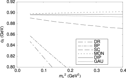
Figure 12: Extrapolated $c_{0}$ as function of lowest data point. Data points are spaced $0.05\,{\rm GeV}^{2}$ apart and the maximum point is $0.8\,{\rm GeV}^{2}$.

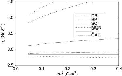
Figure 13: Extrapolated $c_{2}$ as function of lowest data point. Data points are spaced $0.05\,{\rm GeV}^{2}$ apart and the maximum point is $0.8\,{\rm GeV}^{2}$.

It is clear that the dimensionally regularised extrapolation schemes perform poorly. Even with perfect lattice QCD results down to $0.1\,{\rm GeV}^{2}$, $c_{0}$ is likely to be in error by 7% and $c_{2}$ by around 40%. On the other hand, one finds excellent agreement in the chiral parameters, $c_{0}$ and $c_{2}$, obtained from the finite-ranged regulators, even with the lowest data point situated at $0.4\,{\rm GeV}^{2}$. This indicates that, using the technique of finite-range regularisation, one should be able to extract chiral coefficients at the 1% level from the lattice QCD data which will be obtained in the next few years.

Appendix A Renormalisation

Here we summarise the renormalisation prescription for various regularisation schemes. There are two types of diagrams which need to be considered in this analysis. The first of these is the $NN\pi$-type diagram, while the second corresponds to the case of a non-degenerate intermediate state, like the $N\Delta\pi$.

Within the heavy-baryon, non-relativistic approximation the integral describing the $N\to N\pi$ diagram is written as

$$I_{\pi}=\frac{2}{\pi}\int_{0}^{\infty}dk\,\frac{k^{4}\,u^{2}(k)}{k^{2}+m^{2}}\,,$$ (7)

where the factor $u(k)$ is the $N\pi$ vertex regulator. The integral has been defined in such a way that the coefficient of the $m_{\pi}^{3}$ contribution is normalised to unity. For the off-diagonal contribution the loop-integral can be expressed as

$$I_{\pi\Delta}=\frac{2}{\pi}\int_{0}^{\infty}dk\,\frac{k^{4}\,u^{2}(k)}{\sqrt{k^{2}+m^{2}}(\Delta+\sqrt{k^{2}+m^{2}})}\,,$$ (8)

with $\Delta$ the $\Delta$–$N$ mass-splitting, defined as positive for a heavier intermediate state. The normalisation is chosen to agree with the previous equation in the limit $\Delta\to 0$. The various functional forms for the finite-ranged regulators are listed in the text.

Independent of the regulator, the Taylor expansion of the integral, $I_{\pi}$, behaves as

$$I_{\pi}(m\sim 0)=b_{0}+b_{2}m^{2}+m^{3}+b_{4}m^{4}+\dots$$ (9)

With the intermediate state being non-degenerate, the $m^{3}$ contribution becomes a logarithm and the expansion is given by

$$I_{\pi\Delta}(m\sim 0)= b_{0\Delta}+b_{2\Delta}m^{2}+b_{4\Delta}m^{4}$$ (10)

$$-\frac{3}{4\,\pi\,\Delta}m^{4}\log m+\ldots$$

With respect to the chiral expansion, Eq. (1), the self-energy contributions giving rise to the LNA and NLNA are given by

$$\sigma_{{\rm N}\pi}(m_{\pi},\Lambda) = C_{N}\,I_{\pi}(m_{\pi},\Lambda)\,,$$

$$\sigma_{\Delta\pi}(m_{\pi},\Lambda) = C_{\Delta}\,I_{\pi\Delta}(m_{\pi},\Lambda)\,,$$ (11)

where for simplicity we have defined $C_{N}=c_{LNA}$ and $C_{\Delta}=-c_{NLNA}4\pi\Delta/3$. The renormalisation to obtain the low-energy constants of the Taylor expansion, Eq. (2), is then simply given by

$$c_{0} = a_{0}+C_{N}\,b_{0}+C_{\Delta}\,b_{0\Delta}\,,$$

$$c_{2} = a_{2}+C_{N}\,b_{2}+C_{\Delta}\,b_{2\Delta}\,,$$

$$c_{4} = a_{4}+C_{N}\,b_{4}+C_{\Delta}\,b_{4\Delta}\,.$$ (12)

It is these renormalised coefficients, $c_{i}$, which have physical significance and it is these that should be compared with phenomenological studies of chiral expansions.

In Table 3 we summarise the $b_{i}$ expansion coefficients. We were unable to obtain neat analytic expressions for the Gaussian regulator and hence all relevant calculations have been performed numerically. For both DR and BP schemes the $b_{i}$ of the $I_{\pi}$ diagram can trivially be treated as zero.

Regulator	$b_{0}$	$b_{2}$	$b_{4}$
Sharp	$\frac{2\Lambda^{3}}{3\pi}$	$-\frac{2\Lambda}{\pi}$	$-\frac{2}{\pi\Lambda}$
Monopole	$\frac{\Lambda^{3}}{2}$	$-\frac{\Lambda}{2}$	$-\frac{3}{2\Lambda}$
Dipole	$\frac{\Lambda^{3}}{16}$	$-\frac{5\Lambda}{16}$	$-\frac{35}{16\Lambda}$

Table 3: Expansion coefficients for the finite regulators.

The expansion terms, $b_{i\,\Delta}$ for the $I_{\pi\Delta}$ diagram are more complicated and are summarised in the following.

In the DR case, the $b_{i\,\Delta}$ can again be treated as zero. From the expansion of Eq. (4), for the BP case one finds that the appropriate coefficients are given by (with renormalisation scale $1.0\,{\rm GeV}$)

$$b_{0\Delta}^{\rm BP} = \frac{\Delta^{3}}{\pi}\,\log(4\Delta^{2})\,,$$

$$b_{2\Delta}^{\rm BP} = -\frac{\Delta}{2\,\pi}\,\left[1+3\log(4\Delta^{2})\right]\,,$$

$$b_{4\Delta}^{\rm BP} = \frac{3}{16\,\pi\,\Delta}\,\left[3+4\log 2+2\log(\Delta^{2})\right]\,.$$ (13)

For the sharp cut-off, expressions are given by

$$b_{0\Delta}^{\rm SC} = \frac{1}{3\pi}\left[6\Delta^{2}\Lambda-3\Delta\Lambda^{2}+2\Lambda^{3}+6\Delta^{3}\log{\frac{\Delta}{\Delta+\Lambda}}\right]\,,$$

$$b_{2\Delta}^{\rm SC} = \frac{1}{\pi(\Delta+\Lambda)}\left[-\Lambda(3\Delta+2\Lambda)-3\Delta(\Delta+\Lambda)\log{\frac{\Delta}{\Delta+\Lambda}}\right]\,,$$

$$b_{4\Delta}^{\rm SC} = \frac{-1}{16\pi\Delta(\Delta+\Lambda)^{2}}\left[7\,\Delta^{2}+2\,\Delta\,\Lambda-9\,\Lambda^{2}+12\,(\Delta+\Lambda)^{2}\,\log{\frac{\Delta+\Lambda}{2\,\Delta\,\Lambda}}\right]\,.$$ (14)

For the monopole we obtain

$$b_{0\Delta}^{\rm MON} = \frac{\Lambda^{4}}{2\,\pi(\Delta^{2}+\Lambda^{2})^{2}}\left[-2\,\Delta^{3}-2\,\Delta\,\Lambda^{2}+3\,\Delta^{2}\,\Lambda\,\pi+\Lambda^{3}\,\pi+2\,\Delta^{3}\,\log\left(\frac{\Delta^{2}}{\Lambda^{2}}\right)\right]\,,$$

$$b_{2\Delta}^{\rm MON} = -\frac{\Lambda^{2}}{2\,\pi(\Delta^{2}+\Lambda^{2})^{3}}\Bigg{[}\Delta^{5}+6\,\Delta^{3}\,\Lambda^{2}+5\,\Delta\,\Lambda^{4}-3\,\Delta^{2}\,\Lambda^{3}\,\pi+\Lambda^{5}\,\pi$$

$$\hskip 19.91692pt-2\,\Delta\,\Lambda^{2}\,\left(\Delta^{2}-3\,\Lambda^{2}\right)\,\log\left(\frac{\Delta}{\Lambda}\right)\Bigg{]}\,,$$

$$b_{4\Delta}^{\rm MON} = -\frac{1}{16\,\pi\,\Delta(\Delta^{2}+\Lambda^{2})^{4}}\Bigg{[}13\,\Delta^{8}+54\,\Delta^{6}\,\Lambda^{2}+108\,\Delta^{4}\,\Lambda^{4}+58\,\Delta^{2}\,\Lambda^{6}-9\,\Lambda^{8}-24\,\Delta^{3}\,\Lambda^{5}\,\pi$$ (15)

$$\hskip 19.91692pt+24\,\Delta\,\Lambda^{7}\,\pi-6\,\Lambda^{4}\,\left(\Delta^{4}-6\,\Delta^{2}\,\Lambda^{2}+\Lambda^{4}\right)\,\log\left(4\Delta^{2}\right)$$

$$\hskip 19.91692pt-6\,\left(\Delta^{8}+4\,\Delta^{6}\,\Lambda^{2}+5\,\Delta^{4}\,\Lambda^{4}+10\,\Delta^{2}\,\Lambda^{6}\right)\,\log\left(4\Lambda^{2}\right)\Bigg{]}\,.$$

For the dipole we obtain

$$b_{0\Delta}^{\rm DIP} = \frac{\Lambda^{4}}{48\pi(\Delta^{2}+\Lambda^{2})^{4}}\Bigg{[}8\,\Delta^{7}+48\,\Delta^{5}\,\Lambda^{2}+24\,\Delta^{3}\,\Lambda^{4}-16\,\Delta\,\Lambda^{6}-3\,\Delta^{6}\,\Lambda\,\pi$$

$$\hskip 19.91692pt-27\,\Delta^{4}\,\Lambda^{3}\,\pi+27\,\Delta^{2}\,\Lambda^{5}\,\pi+3\,\Lambda^{7}\,\pi+96\,\Delta^{3}\,\Lambda^{4}\,\log{\frac{\Delta}{\Lambda}}\Bigg{]}\,,$$

$$b_{2\Delta}^{\rm DIP} = -\frac{\Lambda^{2}}{48\pi(\Delta^{2}+\Lambda^{2})^{5}}\Bigg{[}8\,\Delta^{9}+36\,\Delta^{7}\,\Lambda^{2}+36\,\Delta^{5}\,\Lambda^{4}+188\,\Delta^{3}\,\Lambda^{6}+180\,\Delta\,\Lambda^{8}+3\,\Delta^{6}\,\Lambda^{3}\,\pi$$

$$\hskip 19.91692pt+45\,\Delta^{4}\,\Lambda^{5}\,\pi-135\,\Delta^{2}\,\Lambda^{7}\,\pi+15\,\Lambda^{9}\,\pi-48\,\left(5\,\Delta^{3}\,\Lambda^{6}-3\,\Delta\,\Lambda^{8}\right)\,\log{\frac{\Delta}{\Lambda}}\Bigg{]}\,,$$

$$a_{4\Delta}^{\rm DIP} = \frac{-1}{48\,\Delta\,{\left(\Delta^{2}+\Lambda^{2}\right)}^{6}\,\pi}\Bigg{[}54\,\Delta^{12}+326\,\Delta^{10}\,\Lambda^{2}+819\,\Delta^{8}\,\Lambda^{4}+1062\,\Delta^{6}\,\Lambda^{6}+1154\,\Delta^{4}\,\Lambda^{8}$$ (16)

$$\hskip 19.91692pt+612\,\Delta^{2}\,\Lambda^{10}-27\,\Lambda^{12}+3\,\Delta^{7}\,\Lambda^{5}\,\pi+63\,\Delta^{5}\,\Lambda^{7}\,\pi-315\,\Delta^{3}\,\Lambda^{9}\,\pi+105\,\Delta\,\Lambda^{11}\,\pi$$

$$\hskip 19.91692pt-6\,\Lambda^{8}\,\bigg{(}35\,\Delta^{4}-42\,\Delta^{2}\,\Lambda^{2}+3\,\Lambda^{4}\bigg{)}\,\log\left(4\Delta^{2}\right)-6\,\Delta^{2}\,\bigg{(}3\,\Delta^{10}+18\,\Delta^{8}\,\Lambda^{2}$$

$$\hskip 19.91692pt+45\,\Delta^{6}\,\Lambda^{4}+60\,\Delta^{4}\,\Lambda^{6}+10\,\Delta^{2}\,\Lambda^{8}+60\,\Lambda^{10}\bigg{)}\,\log\left(4\Lambda^{2}\right)\Bigg{]}\,.$$

Finally, we give the full expressions for the finite-range regulated integrals. For the simple diagram, $I_{\pi}$, we obtain

$$I_{\pi}^{\rm SC} = \frac{2\Lambda^{3}}{3\pi}-\frac{2\Lambda}{\pi}m^{2}+\frac{2}{\pi}m^{3}\,\arctan\left(\frac{\Lambda}{m}\right)\,,$$ (17)

$$I_{\pi}^{\rm MON} = \frac{\Lambda^{4}(2m+\Lambda)}{2(m+\Lambda)^{2}}\,,$$ (18)

$$I_{\pi}^{\rm DIP} = \frac{\Lambda^{5}(m^{2}+4m\Lambda+\Lambda^{2})}{16(m+\Lambda)^{4}}\,.$$ (19)

For the more complicated integral, $I_{\pi\Delta}$, we obtain for the sharp cut-off

$$I_{\pi\Delta}^{\rm SC} = \frac{1}{3\pi}\Bigg{\{}6\Delta^{2}\Lambda+2\Lambda^{3}-6\Lambda m^{2}-3\Delta\Lambda{\sqrt{\Lambda^{2}+m^{2}}}+3\Delta\left(-2\Delta^{2}+3m^{2}\right)\log(\frac{\Lambda+{\sqrt{\Lambda^{2}+m^{2}}}}{m})$$ (20)

$$\hskip 19.91692pt-6{\left(\Delta^{2}-m^{2}\right)}^{\frac{3}{2}}\Bigg{[}\log\left(\frac{-\Delta-m+{\sqrt{\Delta^{2}-m^{2}}}}{\Delta+m+{\sqrt{\Delta^{2}-m^{2}}}}\right)$$

$$\hskip 19.91692pt+\log\left(\frac{\Delta+\Lambda+{\sqrt{\Delta^{2}-m^{2}}}+{\sqrt{\Lambda^{2}+m^{2}}}}{-\Delta-\Lambda+{\sqrt{\Delta^{2}-m^{2}}}-{\sqrt{\Lambda^{2}+m^{2}}}}\right)\Bigg{]}\Bigg{\}}\,.$$

For the monopole regulated integral we obtain

$$I_{\pi\Delta}^{\rm MON} = \frac{\Lambda^{4}}{2\pi(\Lambda^{2}+\Delta^{2}-m^{2})^{2}}$$ (21)

$$\Bigg{[}\frac{\Lambda(3\pi m^{4}+m^{2}(-3\pi\Delta^{2}+2\Delta\Lambda-4\pi\Lambda^{2})+\Lambda(-2\Delta^{3}+3\pi\Delta^{2}\Lambda-2\Delta\Lambda^{2}+\pi\Lambda^{3}))}{\Lambda^{2}-m^{2}}$$

$$-2(\Delta^{2}-m^{2})^{3/2}\log\left(\frac{\Delta-\sqrt{\Delta^{2}-m^{2}}}{\Delta+\sqrt{\Delta^{2}-m^{2}}}\right)$$

$$+\frac{\Delta\Lambda(3m^{4}+2\Delta^{2}\Lambda^{2}-3m^{2}(\Lambda^{2}+\Delta^{2}))}{(\Lambda^{2}-m^{2})^{3/2}}\log\left(\frac{\Lambda-\sqrt{\Lambda^{2}-m^{2}}}{\Lambda+\sqrt{\Lambda^{2}-m^{2}}}\right)\Bigg{]}\,.$$

For the dipole regulated integral we obtain

$$I_{\pi\Delta}^{\rm DIP} = \frac{\Lambda^{5}}{48\,{\left(\Lambda^{2}-m^{2}\right)}^{\frac{7}{2}}\,{\left(\Delta^{2}+\Lambda^{2}-m^{2}\right)}^{4}\,\pi}\Bigg{\{}{\sqrt{\Lambda^{2}-m^{2}}}$$ (22)

$$\Bigg{[}-16\,\Delta\,\Lambda^{11}+4\,\Delta\,\Lambda^{9}\,\left(6\,\Delta^{2}-11\,m^{2}\right)+6\,\Delta\,\Lambda\,m^{4}\,{\left(-\Delta^{2}+m^{2}\right)}^{3}$$

$$+2\,\Delta\,\Lambda^{3}\,m^{2}\,{\left(-\Delta^{2}+m^{2}\right)}^{2}\left(-16\,\Delta^{2}+37\,m^{2}\right)$$

$$+6\,\Delta\,\Lambda^{7}\,\left(8\,\Delta^{4}-44\,\Delta^{2}\,m^{2}+37\,m^{4}\right)$$

$$-2\,\Delta\,\Lambda^{5}\,\left(-\Delta+m\right)\,\left(\Delta+m\right)\,\left(4\,\Delta^{4}-98\,\Delta^{2}\,m^{2}+121\,m^{4}\right)$$

$$+3\,\Lambda^{12}\,\pi-3\,m^{6}\,{\left(-\Delta^{2}+m^{2}\right)}^{3}\,\pi-9\,\Lambda^{10}\,\left(-3\,\Delta^{2}+4\,m^{2}\right)\,\pi$$

$$+9\,\Lambda^{2}\,m^{4}\,{\left(-\Delta^{2}+m^{2}\right)}^{2}\,\left(-\Delta^{2}+4\,m^{2}\right)\,\pi$$

$$-9\,\Lambda^{4}\,m^{2}\,\left(-\Delta+m\right)\,\left(\Delta+m\right)\,\left(\Delta^{4}-11\,\Delta^{2}\,m^{2}+7\,m^{4}\right)\,\pi$$

$$+9\,\Lambda^{8}\,\left(-3\,\Delta^{4}-3\,\Delta^{2}\,m^{2}+7\,m^{4}\right)\,\pi$$

$$-3\,\Delta^{2}\,\Lambda^{6}\,\left(\Delta^{4}-30\,\Delta^{2}\,m^{2}+30\,m^{4}\right)\,\pi\Bigg{]}$$

$$-48\,\Lambda^{3}\,{\left(\Delta^{2}-m^{2}\right)}^{\frac{3}{2}}\,{\left(\Lambda^{2}-m^{2}\right)}^{\frac{7}{2}}\,\log\left(\frac{\Delta-{\sqrt{\Delta^{2}-m^{2}}}}{\Delta+{\sqrt{\Delta^{2}-m^{2}}}}\right)$$

$$-3\,\Delta\,\Bigg{[}m^{6}\,{\left(-\Delta^{2}+m^{2}\right)}^{3}+8\,\Lambda^{10}\,\left(-2\,\Delta^{2}+3\,m^{2}\right)$$

$$-3\,\Lambda^{2}\,m^{4}\,{\left(-\Delta^{2}+m^{2}\right)}^{2}\,\left(-2\,\Delta^{2}+5\,m^{2}\right)$$

$$-4\,\Lambda^{8}\,m^{2}\,\left(-14\,\Delta^{2}+15\,m^{2}\right)+\Lambda^{6}\,m^{4}\,\left(-34\,\Delta^{2}+35\,m^{2}\right)$$

$$+3\,\Lambda^{4}\,m^{4}\,\left(8\,\Delta^{4}-13\,\Delta^{2}\,m^{2}+5\,m^{4}\right)\Bigg{]}\,\log\left(\frac{\Lambda-{\sqrt{\Lambda^{2}-m^{2}}}}{\Lambda+{\sqrt{\Lambda^{2}-m^{2}}}}\right)\Bigg{\}}\,.$$

References

- (1) W. Detmold et al., Pramana 57 (2001) 251, nucl-th/0104043.
- (2) D.B. Leinweber and T.D. Cohen, Phys. Rev. D47 (1993) 2147, hep-lat/9211058.
- (3) D.B. Leinweber and T.D. Cohen, Phys. Rev. D49 (1994) 3512, hep-ph/9307261.
- (4) D.B. Leinweber, D.H. Lu and A.W. Thomas, Phys. Rev. D60 (1999) 034014, hep-lat/9810005; E.J. Hackett-Jones, D.B. Leinweber and A.W. Thomas, Phys. Lett. B489 (2000) 143, hep-lat/0004006; E.J. Hackett-Jones, D.B. Leinweber and A.W. Thomas, Phys. Lett. B494 (2000) 89, hep-lat/0008018; D.B. Leinweber, A.W. Thomas and R.D. Young, Phys. Rev. Lett. 86 (2001) 5011, hep-ph/0101211; T.R. Hemmert and W. Weise, hep-lat/0204005.
- (5) D.B. Leinweber et al., Phys. Rev. D61 (2000) 074502, hep-lat/9906027; D.B. Leinweber, A.W. Thomas and S.V. Wright, Phys. Lett. B482 (2000) 109, hep-lat/0001007; D.B. Leinweber et al., Phys. Rev. D64 (2001) 094502, arXiv:hep-lat/0104013; S.V. Wright et al., Nucl. Phys. Proc. Suppl. 109 (2002) 50, hep-lat/0111053.
- (6) W. Detmold et al., Phys. Rev. Lett. 87 (2001) 172001, hep-lat/0103006; W. Detmold, W. Melnitchouk and A.W. Thomas, Phys. Rev. D66 (2002) 054501, hep-lat/0206001.
- (7) D.B. Leinweber and A.W. Thomas, Phys. Rev. D62 (2000) 074505, hep-lat/9912052; R. Lewis, W. Wilcox and R.M. Woloshyn, hep-ph/0210064.
- (8) X.H. Guo and A.W. Thomas, Phys. Rev. D65 (2002) 074019, hep-ph/0112040.
- (9) R.D. Young et al., Phys. Rev. D66 (2002) 094507, hep-lat/0205017; R.D. Young et al., Proceedings of the Workshop on Physics at the Japan Hadron Facility (JHF) (2002) 155, nucl-th/0211026.
- (10) J.F. Donoghue, B.R. Holstein and B. Borasoy, Phys. Rev. D59 (1999) 036002, hep-ph/9804281.
- (11) C. Bernard et al., (2002), hep-lat/0209086.
- (12) M. Gell-Mann, R.J. Oakes and B. Renner, Phys. Rev. 175 (1968) 2195.
- (13) L.F. Li and H. Pagels, Phys. Rev. Lett. 26 (1971) 1204.
- (14) B. Borasoy et al., Phys. Rev. D66 (2002) 094020, hep-ph/0210092.
- (15) J. Gasser, M.E. Sainio and A. Svarc, Nucl. Phys. B307 (1988) 779.
- (16) R.F. Lebed, Nucl. Phys. B430 (1994) 295, hep-ph/9311234.
- (17) M.K. Banerjee and J. Milana, Phys. Rev. D54 (1996) 5804, hep-ph/9508340.
- (18) S.V. Wright, PhD thesis, University of Adelaide, 2002.
- (19) I.C. Cloet, D.B. Leinweber and A.W. Thomas, Phys. Rev. C65 (2002) 062201, hep-ph/0203023.
- (20) CP-PACS, A. Ali Khan et al., Phys. Rev. D65 (2002) 054505, hep-lat/0105015.
- (21) Y. Iwasaki, Nucl. Phys. B258 (1985) 141.
- (22) UKQCD, C.R. Allton et al., Phys. Rev. D60 (1999) 034507, hep-lat/9808016.
- (23) R. Sommer, Nucl. Phys. B411 (1994) 839, hep-lat/9310022.
- (24) R.G. Edwards, U.M. Heller and T.R. Klassen, Nucl. Phys. B517 (1998) 377, hep-lat/9711003.
- (25) T. Becher and H. Leutwyler, Eur. Phys. J. C9 (1999) 643, hep-ph/9901384.
- (26) C. Bernard et al., Phys. Rev. D64 (2001) 054506, hep-lat/0104002.
- (27) J.A. McGovern and M.C. Birse, Phys. Lett. B446 (1999) 300, hep-ph/9807384.