1 Introduction

QCD exhibits two remarkable features, confinement and chiral symmetry breaking, which both are cornerstones for our understanding of strongly interacting particles. It is an interesting property of QCD that at the QCD phase transition the restoration of chiral symmetry and the disappearance of confinement occur at the same critical temperature. This seems to indicate that the two phenomena are intimately linked with each other. So far the two phenomena have resisted our attempts to find a description unifying them and the structure of the fundamental excitations of the QCD vacuum is still unclear.

In recent years lattice calculations have started to contribute to our understanding of the QCD vacuum fluctuations. In particular it was found that the eigenmodes of the Dirac operator provide a powerful filter removing the hard UV fluctuations and only the long range modes couple to the low eigenvectors [1]-[4]. These studies were inspired by the phenomenological picture of chiral symmetry breaking based on instantons [5]. In this picture the QCD vacuum is described as a fluid of interacting instantons and anti-instantons. Instead of a zero-mode which exists for a single instanton [6, 7] the fluid of interacting instantons and anti-instantons gives rise to many near zero-modes which have small but non-zero eigenvalues. The density of these eigenvalues is then related to the chiral condensate by the Banks-Casher formula [8]. Lattice studies have established that the near zero-modes do indeed show a lumpy structure and are locally chiral as expected from the instanton picture. Furthermore it was demonstrated that the lumps in the field strength have a high degree of self-duality [3]. Note however, that first attempts to fit eigenmodes of the Dirac operator with the profile of the ’t Hooft zero-mode have failed [4].

In this article we use a new method for probing the QCD vacuum with eigenvectors of the lattice Dirac operator. We introduce an arbitrary phase $\exp(i2\pi\zeta)$ with $\zeta\in[0,1]$ at the temporal boundary of the Dirac operator and analyze how the zero-mode in configurations with topological charge $Q=\pm 1$ responds to changes in $\zeta$. The most prominent feature we discover is that the zero-mode changes its position and can be located at different space-time points for different values of $\zeta$. This property is observed for quenched ensembles of SU(3) gauge configurations with temperature, both in the confined and the deconfined phase as well as for configurations on a torus.

Our generalized boundary condition is motivated by an interesting property of zero-modes for Kraan-van Baal (KvB) solutions of the classical Yang-Mills equations on a euclidean cylinder. KvB solutions [9] generalize the caloron solution [10] by allowing for non-trivial Polyakov loop at spatial infinity. KvB solutions depend in addition to the phases of the Polyakov loop at spatial infinity also on $N$ (for SU($N$)) vectors $\vec{y}_{i},i=1,2\,...\,N$. When one draws apart those vectors one finds that an object of charge 1 is built from $N$ constituent monopoles and this property might lead to the missing link between confinement and chiral symmetry breaking. Strong evidence for SU(2) KvB solutions in cooled lattice gauge configurations were given for twisted [11] and periodic boundary conditions [12].

For KvB solutions also the zero-mode has been computed [13]. This zero-mode has the remarkable property that it is located on only one of the constituent monopoles but it can jump from one monopole to another when changing $\zeta$. In a previous article [14] we have compared zero-modes with periodic and anti-periodic boundary conditions and have found clear signals for KvB-type behavior. Here we now use the generalized boundary condition with phase $\exp(i2\pi\zeta)$ and present further strong evidence that the excitations of QCD at high temperature have the structure of KvB solutions.

In a subsequent step we apply the techniques that were successful in detecting the constituent monopoles at high temperature to gauge configurations generated on a torus. For the torus no equivalent of KvB solutions is known. However, several articles have put forward the idea that also at low temperatures constituents with fractional charge build up lumps with integer topological charge [15]. Our finding, that when changing the fermionic boundary condition the zero-mode does change its position, indicates that indeed an excitation with topological charge $|Q|$ = 1 is built from several separate lumps.

2 Technicalities

2.1 Gauge configurations

For our runs we use gauge ensembles generated with the Lüscher-Weisz action [16] with coefficients from tadpole improved perturbation theory. We work at two different values of the inverse gauge coupling $\beta=8.20$ and $\beta=8.45$. A determination of the lattice spacing based on the Sommer parameter gives $a=0.115(1)$ fm and $a=0.094(1)$ respectively [17].

At those two couplings we generate configurations on $6\times 20^{3}$ lattices. The two values of $\beta$ then give rise to an ensemble in the confining phase ($\beta=8.20$) and an ensemble in the deconfined phase ($\beta=8.45$). The corresponding temperatures are 287 and 350 MeV. The critical temperature for the QCD phase transition was determined as $T_{c}=300$ MeV for the Lüscher-Weisz action [18].

We restrict ourselves to configurations with topological charge $Q=\pm 1$, by considering configurations with a single zero-mode. Thus problems with mixing of different zero-modes are avoided. From two larger samples of typically 400 configurations we selected 70 configurations with charge $Q=\pm 1$ for $\beta=8.20$ and 89 configurations for $\beta=8.45$.

For the deconfined ensemble ($\beta=8.45$) the Polyakov loop has a non-vanishing expectation value. Due to the $Z_{3}$ symmetry of the gauge action the Polyakov loop can come with three different values for its phase $\varphi=0,\pm 2\pi/3$. The Dirac operator does not have this symmetry and thus the eigenvectors and eigenvalues of the Dirac operator will behave differently for real, respectively complex Polyakov loop. We found that of the 89 configurations in the deconfined phase 25 have real Polyakov loop and 64 have $\varphi=\pm 2\pi/3$. In the following we will often refer to these two subsets as the real and complex sector.

Finally we also generated a low temperature ensemble on $16^{4}$ lattices at $\beta=8.45$. It consists of 46 configurations. For all ensembles we use periodic boundary conditions for the gauge fields. In Table 1 we summarize the parameters of our ensembles. We quote the lattice size, the inverse gauge coupling, the statistics, the lattice spacing and the temperature in MeV as well as in units of $T_{c}$. We formally asign also a temperature to the $16^{4}$ ensemble even though no temporal direction is distinguished by the lattice geometry.

size	$\beta$	statistics	$a$ [fm]	$T$ [MeV]	$T/T_{c}$
$6\times 20^{3}$	8.45	64 + 25	0.094(1)	350	1.17
$6\times 20^{3}$	8.20	70	0.115(1)	287	0.96
$16^{4}$	8.45	46	0.094(1)	113	0.44

Table 1: Parameters of our gauge ensembles.

2.2 Observables

As already outlined in the introduction we use the eigenvectors of the Dirac operators to analyze excitations of the QCD vacuum since they provide an excellent filter removing the UV fluctuations. Here we use the chirally improved operator [19]. The chirally improved Dirac operator is a systematic expansion of a solution of the Ginsparg-Wilson equation [20] and has very good chiral properties. It has been successfully used for quenched spectroscopy [21] with pion masses down to 230 MeV. In [22] it was shown, that chirally improved fermions reproduce the analytic result for the zero-mode in the background of a discretized instanton very well. In particular for small instanton radii it is considerably more accurate than the overlap operator.

We compute the eigenvectors and eigenvalues of the chirally improved Dirac operator using the implicitly restarted Arnoldi method [23]. For the fermions we use periodic boundary conditions for the spatial directions. In time direction we implement general boundary conditions that allow for an arbitray phase,

$$\psi(N_{t}+1,\vec{x})\;\;=\;\;\exp(\,i\,2\pi\,\zeta)\,\psi(1,\vec{x})\;.$$ (2.1)

By $N_{t}$ we denote the number of lattice points in time direction. The parameter $\zeta$ can assume values in the interval [0,1], with $\zeta=0$ corresponding to periodic temporal boundary conditions and $\zeta=0.5$ giving the anti-periodic case. Note that the value $\zeta=1$ gives the same boundary condition as $\zeta=0$. For all of our configurations as listed in Table 1 we computed eigenmodes for periodic and anti-periodic temporal boundary conditions. For smaller subsets from each ensemble we also computed eigenvectors for smaller steps in $\zeta$, such as $\zeta=0.1,0.2\,...$ . More detailed information on these configurations is listed in tables below.

From the eigenvectors $\psi$ we construct several gauge invariant observables. The simplest observable is the scalar density $\rho(x)$ of the eigenvectors obtained by summing color and Dirac indices $c,d$ for each space-time point $x$ separately,

$$\rho(x)\;\;=\;\;\sum_{c,d}|\psi(x)_{c,d}|^{2}\;.$$ (2.2)

Note that since our eigenvectors $\psi$ are normalized one has $\sum_{x}\rho(x)=1$ where the sum runs over all lattice points $x$. From the analytic continuum result as well as from lattice studies it is known that the zero-mode traces the underlying instanton. Plots of the density $\rho(x)$ for slices of the lattice will be used below to illustrate the behavior of the eigenmodes. We will also compare the position of the lumps seen by different eigenmodes $\psi_{1},\psi_{2}$ by computing the euclidean 4-distance $d_{4}$ between their maxima

$$d_{4}\;\;=\;\;\parallel x^{max}_{1}-x^{max}_{2}\parallel\;,$$ (2.3)

where $x^{max}_{1}$ and $x^{max}_{2}$ are the lattice points with the largest values of the density for $\psi_{1}$, respectively $\psi_{2}$.

In order to quantify the localization of the lump seen by the eigenmode we use the so-called inverse participation ratio defined as

$$I\;\;=\;\;V\sum_{x}\rho(x)^{2}\;,$$ (2.4)

where $V$ denotes the total number of lattice points. If a mode is localized on a single site $x_{0}$ ($\rho(x)=\delta_{x,x_{0}}$) then one finds $I=V$. For an entirely spread out mode ($\rho(x)=1/V$ for all $x$) one has $I=1$. Thus localized modes have large $I$, while delocalized modes have small values of $I$.

Finally we describe an observable to characterize the overlap of lumps seen by different eigenmodes. In particular we compute the overlap of the support of the two lumps seen by eigenvectors $\psi_{1}$ and $\psi_{2}$. The support is defined as the function $\theta(x)$ which has $\theta(x)=1$ for the lattice points $x$ carrying the lump in $\rho$ and $\theta(x)=0$ for all other points. An open question is how to identify the lump. For a narrow lump the support is small while a broad lump has a much larger support. Using the inverse participation ratio $I$ we define a number $N=$ Int$[V/(32I)+1]$ and use this to determine the support by setting $\theta(x)=1$ for those $N$ lattice points $x$ which carry the $N$ largest values of $\rho$ and $\theta(x)=0$ for all other points. The normalization of $N$ is chosen such that if the lump was a 4-D Gaussian the support would consist of the 4-volume carrying the points inside the half-width of the Gaussian. Note that $N$ is the size of the support, i.e. $N=\sum_{x}\theta(x)$.

With our definition of the support of the two lumps ($\theta_{1}$ for eigenvector $\psi_{1}$, $\theta_{2}$ for eigenvector $\psi_{2}$) we can define the overlap function $C$ of the two lumps as

$$C(x)\;\;=\;\;\theta_{1}(x)\theta_{2}(x)\;.$$ (2.5)

From $C(x)$ we compute the relative overlap

$$R_{12}\;\;=\;\;\frac{2}{N_{1}\,+\,N_{2}}\;\sum_{x}C(x)\;.$$ (2.6)

The relative overlap $R_{12}$ is a real number ranging from 0 to 1. If the lump in $\rho_{1}$ and the lump in $\rho_{2}$ sit on top of each other (at least the core up to about the half-width) and have the same size then $R_{12}=1$. If the two lumps are entirely separated one has $R_{12}=0$. Values in between give the ratio of the common volume of the two supports to the average size of the two supports. Note that even if the two lumps sit on top of each other, but have different sizes $N_{1},N_{2}$ one has $R_{12}<1$.

3 A few words on Kraan - van Baal solutions

When we present our data in the sections below we will show that the two ensembles with finite temperature, i.e. the runs on the $6\times 20^{3}$ lattices, can be described by Kraan - van Baal (KvB) solutions. In order to facilitate this enterprise let us briefly discuss the structure of the KvB solutions [9] and the analytic results for the corresponding zero-mode [13].

3.1 Kraan - van Baal solutions

Kraan van-Baal solutions are classical solutions of the Yang-Mills equations on a euclidean cylinder. They are characterized by the Polyakov loop at spatial infinity ${\cal P}_{\infty}$ given by

$${\cal P}_{\infty}\;\;=\;\;\lim_{|\vec{x}|\rightarrow\infty}P\,\exp\left(\int_{0}^{\beta}dtA_{0}(t,\vec{x})\right)\;,$$ (3.7)

where $\beta$ is the time extent of the cylinder and the temporal boundary conditions of the gauge field are periodic, i.e. $A_{\mu}(\beta+t,\vec{x})=A_{\mu}(t,\vec{x})$. With a suitable constant gauge transformation ${\cal P}_{\infty}$ can be diagonalized and is given by (we show the formulae for SU(3))

$${\cal P}_{\infty}\;\;=\;\;\exp\Big{(}\,i\,2\pi\,\mbox{diag}(\mu_{1},\mu_{2},\mu_{3})\Big{)}\;.$$ (3.8)

The determinant of ${\cal P}_{\infty}$ has to equal 1 which implies that $\mu_{1}+\mu_{2}+\mu_{3}$ is an integer. In order to have a unique labeling of ${\cal P}_{\infty}$ one chooses the constant gauge transformation and the phases such that

$$\mu_{1}\,+\,\mu_{2}\,+\,\mu_{3}\;\;=\;\;0\;,$$

$$\mu_{1}\;\leq\;\mu_{2}\;\leq\;\mu_{3}\;\leq\;\mu_{4}\;\;\equiv\;\;1+\mu_{1}\;.$$ (3.9)

In the second line we defined another phase factor $\mu_{4}$ which will be useful for a compact notation. Using the scale invariance of the classical equations the time extent $\beta$ can be set to $\beta=1$. Subsequently we use this convention and distances are now expressed in units of $\beta$.

In addition to the phase factors $\mu_{i}$ the KvB solution also depends on 3 spatial vectors $\vec{y}_{1},\vec{y}_{2},\vec{y}_{3}$. As already remarked the KvB solution can be seen to consist of $3$ constituent monopoles and the $\vec{y}_{i}$ are their positions. As for the $\mu_{m}$ we define a 4-th vector $\vec{y}_{4}=\vec{y}_{1}$ for notational convenience. The action density of the KvB solutions can be written as

$$\mbox{Tr}F_{\mu\nu}^{\,2}(x) = \partial_{\mu}^{2}\partial_{\nu}^{2}\log\psi(x)\;,$$

$$\psi(x) = \frac{1}{2}\,\mbox{tr}({\cal A}_{3}\,{\cal A}_{2}\,{\cal A}_{1})\;-\;\cos(2\pi t)\;,$$

$${\cal A}_{m} = \frac{1}{r_{m}}\left(\begin{array}[]{cc}r_{m}&|\vec{y}_{m}-\vec{y}_{m+1}|\\ 0&r_{m+1}\end{array}\right)\left(\begin{array}[]{cc}c_{m}&s_{m}\\ s_{m}&c_{m}\end{array}\right)\;.$$ (3.14)

In these equations $r_{m}=|\vec{x}-\vec{y}_{m}|$, $c_{m}=\cosh(2\pi\nu_{m}r_{m})$ and $s_{m}=\sinh(2\pi\nu_{m}r_{m})$. Each monopole can be assigned a mass $M_{m}$,

$$M_{m}\;\;=\;\;8\pi^{2}\,(\mu_{m+1}-\mu_{m})\;.$$ (3.15)

This expression for the monopole mass $M_{m}$ implies that the $m^{th}$ monopole is localized when $\mu_{m+1}-\mu_{m}$ is large and it is spread out for small $\mu_{m+1}-\mu_{m}$.

In order to illustrate the structure of the KvB solutions we show the corresponding action density for an example in Fig. 1. The values of the parameters are $(\mu_{1},\mu_{2},\mu_{3})=(-17,-2,19)/60$. The positions of the monopoles are chosen as $\vec{y}_{1}=(-2,-2,0)$, $\vec{y}_{2}=(0,2,0)$ and $\vec{y}_{3}=(2,-1,0)$. We show the action density in the $x,y$-plane on a logarithmic scale.

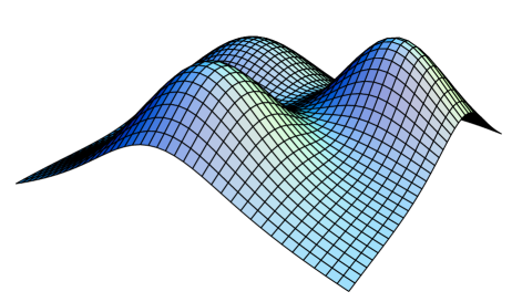
Figure 1: Action density of a typical KvB solution for a $x,y$-slice on a logarithmic scale. The parameters of the solution are $(\mu_{1},\mu_{2},\mu_{3})=(-17,-2,19)/60$, $\vec{y}_{1}=(-2,-2,0)$, $\vec{y}_{2}=(0,2,0)$ and $\vec{y}_{3}=(2,-1,0)$.

3.2 Zero-modes of the Dirac operator

The eigenvalue problem of the Dirac operator in the background of a KvB solution was addressed in [13] and an explicit expression for the zero-mode was given. In particular the problem was solved for general temporal boundary conditions (note that we scaled the temporal extent $\beta$ to $\beta=1$),

$$\psi(1+t,\vec{x})\;\;=\;\;\exp(\,i\,2\pi\,\zeta)\,\psi(t,\vec{x})\;.$$ (3.16)

The density of the zero-mode is given by

$$\rho(x)\;\;=\;\;\sum_{c,d}|\psi(x)_{c,d}|^{2}\;\;=\;\;-\,\frac{1}{(2\pi)^{2}}\,\partial_{\mu}^{2}\hat{f}_{\zeta}(x)\;,$$ (3.17)

with

$$\hat{f}_{\zeta}(x)\;\;=\;\;\frac{\pi}{r_{m}}\,\psi(x)^{-1}\,\langle v^{m}_{\zeta}|{\cal A}_{m-1}\,...\,{\cal A}_{1}{\cal A}_{3}\,...\,{\cal A}_{m}|w^{m}_{\zeta}\rangle\;,$$ (3.18)

and the 2-spinors $|v^{m}_{\zeta}\rangle$ and $|w^{m}_{\zeta}\rangle$ are given by

$$|v^{m}_{\zeta}\rangle\;=\,\left(\!\!\begin{array}[]{c}\sinh(2\pi(\zeta\!-\!\mu_{m})r_{m})\\ \cosh(2\pi(\zeta\!-\!\mu_{m})r_{m})\end{array}\!\!\right),\;|w^{m}_{\zeta}\rangle\;=\,\left(\!\!\begin{array}[]{c}\cosh(2\pi(\zeta\!-\!\mu_{m})r_{m})\\ -\sinh(2\pi(\zeta\!-\!\mu_{m})r_{m})\end{array}\!\!\right).$$ (3.19)

The index $m$ which determines the prefactor $1/r_{m}$, the spinors $|v^{m}_{\zeta}\rangle$, $|w^{m}_{\zeta}\rangle$ and the ordering of the ${\cal A}_{i}$ in Eq. (3.18) as well as the choice of $\mu_{m}$ and $r_{m}$ in Eq. (3.19) is determined from the interval containing the boundary condition parameter,

$$\mu_{m}\;\leq\;\zeta\;\leq\;\mu_{m+1}\;.$$ (3.20)

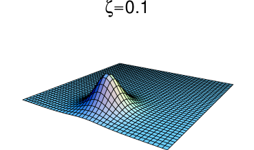
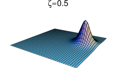
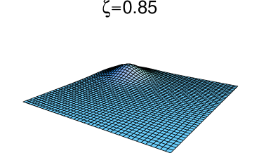
Figure 2: Scalar density of the KvB zero-modes for different values of $\zeta$ in the $x,y$-plane. The parameters are the same as used in Fig. 1, i.e. $(\mu_{1},\mu_{2},\mu_{3})=(-17,-2,19)/60$, $\vec{y}_{1}=(-2,-2,0)$, $\vec{y}_{2}=(0,2,0)$ and $\vec{y}_{3}=(2,-1,0)$.

Before we discuss the implications of this selection rule let us denote a limiting case of the function $\hat{f}_{\zeta}(x)$. In the limit of well separated constituent monopoles, i.e. large $|\vec{y}_{i}-\vec{y}_{i+1}|$ for all $i$ one finds

$$\hat{f}_{\zeta}(x)\;=\;2\pi\,\frac{\sinh(2\pi(\zeta\!-\!\mu_{m})r_{m})\sinh(2\pi(\mu_{m+1}\!-\!\zeta)r_{m})}{r_{m}\,\sinh(2\pi\nu_{m}r_{m})}\;.$$ (3.21)

This limiting case together with the selection rule Eq. (3.20) makes explicit the following two properties of the zero mode:

• The zero mode is located on the $m^{th}$ monopole when the boundary condition parameter $\zeta$ is contained in $[\mu_{m},\mu_{m+1}]$. The position of the lump seen by the zero-mode can jump from $\vec{y}_{m}$ to $\vec{y}_{m+1}$ as the value of $\zeta$ crosses $\mu_{m+1}$.

• The size of the zero-mode depends in addition to the mass of the underlying monopole also on the parameter $\sigma$,

  $$\sigma\;=\;\min\{\,\zeta-\mu_{m}\,,\,\mu_{m+1}-\zeta\,\}\;.$$ (3.22)

  The zero-mode is localized for large values of $\sigma$ and spread-out for small $\sigma$.

In order to demonstrate the features of the zero-modes in Fig. 2 we show plots of the scalar density of the zero-modes for the example where we discussed the action density in the last subsection and displayed the result in Fig. 1. Our example has $(\mu_{1},\mu_{2},\mu_{3},\mu_{4})=(-17,-2,19,43)/60$. This implies that for $\zeta\in[-2/60,19/60]$ the zero mode is located on $y_{2}$, for $\zeta\in[19/60,43/60]$ it is located on $y_{3}$ and for $\zeta\in[43/60,58/60]$ it is located on $y_{1}$. Note that we made use of the equivalence $\zeta\equiv\zeta-1$ in order to treat the interval $[\mu_{1},\mu_{2}]=[-17/60,-2/60]$.

The plots show nicely that indeed the position of the lump seen by the zero-mode can change its position. In the following sections we now make use of this property and use the zero-modes of the lattice Dirac operator with different boundary conditions as a device for detecting different lumps that together build up a topological excitation of charge $Q=\pm 1$.

4 Finite Temperature - results above $T_{c}$

4.1 Overview over the configurations

We remarked in Section 2 that the ensemble in the deconfined phase ($6\times 20^{3}$, $\beta=8.45$) consists of 89 configurations, 25 with real Polyakov loop and 64 with complex Polyakov loop. For a subset of 10 configurations we did not only compute the zero-mode with periodic and anti-periodic temporal boundary conditions but for a general phase $\exp(i2\pi\zeta)$ at the temporal boundary. In particular we studied $\zeta=$ 0.0, 0.1, 0.2, 0.3, 1/3, 0.4, 0.5, 0.6, 2/3, 0.7, 0.8, 0.9. The cases $\zeta=$ 0.0 and $\zeta=$ 0.5 correspond to periodic respectively anti-periodic boundary conditions. For this subset Table 2 lists some basic properties. In particular we list the configuration number, the phase of the Polyakov loop, the inverse participation ratio for the periodic and the anti-periodic zero-mode, the position of the maxima for periodic and anti-periodic b.c., and finally the 4-distance between the two maxima.

conf.	$\varphi$	$I_{P}$	$I_{A}$	$(t,x,y,z)^{max}_{P}$				$(t,x,y,z)^{max}_{A}$				$d_{4}/a$
6	0	2.19	43.16	5	10	9	8	3	4	17	9	10.24
7	$-2\pi/3$	22.81	4.71	3	3	3	11	1	4	2	9	3.16
9	$+2\pi/3$	23.70	5.93	5	8	18	17	5	8	18	17	0.00
10	$+2\pi/3$	40.27	10.04	1	11	13	14	1	11	13	14	0.00
19	0	2.29	20.20	5	11	9	8	4	20	3	8	10.86
38	0	2.38	31.00	5	12	9	8	5	12	9	8	0.00
49	$+2\pi/3$	34.03	15.67	6	11	19	2	6	11	19	2	0.00
87	0	1.90	47.76	6	18	13	9	6	18	13	9	0.00
101	0	2.87	41.69	5	12	18	10	1	19	3	1	12.60
383	0	2.42	42.86	6	19	13	11	2	3	11	4	8.54

Table 2: Parameters of the subensemble in the deconfined phase ($6\times 20^{3}$, $\beta=8.45$) which we studied with finely spaced values for the boundary parameter $\zeta$. For these 10 configurations we quote the configuration number, the phase of the Polyakov loop, the inverse participation ratios $I_{P}$ and $I_{A}$ for the zero-modes with periodic, respectively anti-periodic b.c., the position of the maxima for the corresponding zero-modes and the 4-distance $d_{4}$ between these two maxima in units of the lattice spacing.

A few basic properties of the configurations above $T_{c}$ can be immediately read off from Table 2. For all configurations with real Polyakov loop ($\varphi=0$) the inverse participation ratio of the zero-mode increases when switching from periodic to anti-periodic boundary conditions, i.e. the mode becomes more localized. For the configurations with complex Polyakov loop ($\varphi=\pm 2\pi/3$) the situation is reversed and the state becomes more delocalized when switching from periodic to anti-periodic b.c. Furthermore only configurations with real Polyakov loop allow for a large distance between the lumps seen by the periodic and anti-periodic zero mode. In the following subsections we will elaborate further on these observations.

4.2 Example for the generic behavior

In this subsection we show series of plots of the scalar density for a configuration where we computed with the zero-modes with finely spaced values of $\zeta$. Before we do so let us discuss what can be expected from the analytic KvB result.

In the deconfined phase the Polyakov loop can have the three phases $\varphi=0,\pm 2\pi/3$. Let us first discuss the case of real Polyakov loop. For this case one finds for the phase factors $\mu_{i}$ entering the KvB solutions,

$$(\mu_{1},\mu_{2},\mu_{3},\mu_{4})\;\;=\;\;(0,0,0,1)\;.$$ (4.23)

Applying the rule that the zero mode with boundary factor $\zeta$ is located at position $\vec{y}_{m}$ when $\zeta\in[\mu_{m},\mu_{m+1}]$ we find: For all $\zeta\neq 0$ the zero mode is located on $\vec{y}_{3}$. The only exception is $\zeta=0$ where the zero mode is located on $\vec{y}_{1}$ and $\vec{y}_{2}$. Note that $\zeta=0$ is equivalent to $\zeta=1$ such that also for $\zeta=1$ this second possibility holds. The mode at $\zeta=0,1$ should be very much delocalized, while the other mode seen for $\zeta\neq 0$ is expected to show a changing degree of localization. In particular one expects a rather delocalized mode near the endpoints of the interval $\zeta=0,1$ while it is more localized in the middle of the interval, reaching a maximum of the localization at $\zeta=0.5$.

The plots we will show below are for our configuration 383 from the $6\times 20^{3},\beta=8.45$ ensemble. In Table 3 we show the inverse participation ratio and the position of the maximum of the scalar density for all values of $\zeta$. From the table it is obvious that the mode is located at the same position for all $\zeta\neq 0,1$ and at a different position for $\zeta=0,1$. The distance between the two lumps is $d_{4}/a=8.54$ in lattice units or in fermi $d_{4}=0.80$ fm. The inverse participation ratio is largest near $\zeta=0.5$, i.e. the mode is most localized for anti-periodic boundary conditions. At $\zeta=0,1$ the inverse participation ratio is small and the mode is very much spread out.

$\;\;\zeta$	$I$	$(t,x,y,z)^{max}$				$\;\;\zeta$	$I$	$(t,x,y,z)^{max}$
0.0	2.42	6	9	13	11	0.6	45.32	2	13	11	4
0.1	3.53	2	13	11	4	0.7	35.20	2	13	11	4
0.2	9.15	2	13	11	4	0.8	17.00	2	13	11	4
0.3	19.05	2	13	11	4	0.9	3.40	2	13	11	4
0.4	31.80	2	13	11	4	1.0	2.42	6	9	13	11
0.5	42.86	2	13	11	4

Table 3: Inverse participation ratio and position of the maximum of the scalar density as a function of the boundary condition parameter $\zeta$. The data are for configuration 383 of the deconfined ensemble ($6\times 20^{3},\beta=8.45$). Plots of the corresponding scalar density are shown in Fig. 3.

Let us now look at the plots of the scalar density for configuration 383. In Fig. 3 we show the scalar density on $x,y$-slices of the lattice. In particular we show the slice at $t,z=6,11$ in the left column of plots and the slice at $t,z=2,4$ in the right column of plots. Thus in the left column we show the slice where the scalar density at $\zeta=0,1$ has its peak while in the right column the slice for the maximum at all other values of $\zeta$ is shown. The reason for showing two different slices is that typically for a thermalized configuration the positions of the two maxima do not fall in a common coordinate plane. In the plots we use values of $\zeta=0,0.2$ and 0.5. Note that the scale for the right column differs by a factor of 10 from the scale in the left column.

For $\zeta=0$ there is a clearly visible lump in the 6,11-slice (left column, top plot of Fig. 3), while the 2,4-slice is essentially flat (right column, top plot). As we increase $\zeta$ to $\zeta=0.2$ the peak in the 6,11-slice has vanished, but a small lump in the 2,4-slice has emerged (second row in Fig. 3). This latter lump starts to grow as we increase $\zeta$ and reaches its maximum in the last row of Fig. 3, at $\zeta=0.5$. As we increase $\zeta$ further the lump starts to shrink again, and essentially runs through the series of plots in reverse order. The series of plots shown in Fig. 3 nicely demonstrates that the zero-mode for configuration 383 behaves exactly like the zero-mode for a KvB solution in a deconfined configuration with real Polyakov loop.

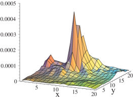
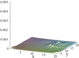
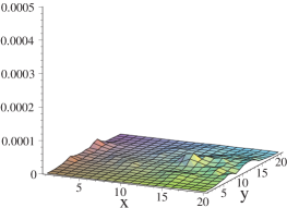
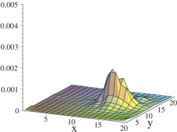
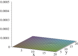
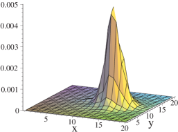
Figure 3: Slices of the scalar density for $6\times 20^{3},\beta=8.45$ and real Polyakov loop (configuration 383). We show $x,y$-slices at $t=6$, $z=11$ (left column) and at $t=2$, $z=4$ (right column). The values for $\zeta$ are $\zeta=0,0.2,0.5$ (from top to bottom). Note the different scale for the l.h.s. and r.h.s. plots.

Let us now look at the other two possibilities for the phase of the Polyakov loop. Phases of $\varphi=2\pi/3$ and $\varphi=-2\pi/3$ correspond to the following two sets of $\mu_{i}$,

$$(\mu_{1},\mu_{2},\mu_{3},\mu_{4})\;\;=\;\;(-2/3,1/3,1/3,1/3)\;,$$ (4.24)

for $\varphi=2\pi/3$ and

$$(\mu_{1},\mu_{2},\mu_{3},\mu_{4})\;\;=\;\;(-1/3,-1/3,2/3,2/3)\;,$$ (4.25)

for $\varphi=-2\pi/3$. Thus for $\varphi=2\pi/3$ the zero-mode has to be located at the same position for all $\zeta\neq 1/3$ and only for $\zeta\in[1/3,1/3]$ (in other words for $\zeta=1/3$) the lump can sit at a different position. For $\varphi=2\pi/3$ the zero-mode has to be located at the same position for all $\zeta\neq 2/3$, but can have a different location for $\zeta=2/3$. This discussion shows that the situation for $\varphi=\pm 2\pi/3$ is equivalent to the $\varphi=0$ case and only the interval $[0,1]$ is shifted, such that the position of a possible jump of the location is shifted to $\zeta=1/3$, respectively $\zeta=2/3$.

We find that all our configurations in the deconfined ensemble obey the general pattern we have discussed. Certainly it is also clear that our thermalized configurations are not classical solutions and quantum effects play a role. For example we find for the configuration shown in Fig. 3 that the peak in the $6,11$-slice is already visible at $\zeta=0.9$. For an unperturbed KvB solution it should be visible only at exactly $\zeta=1$ (equivalent to $\zeta=0$). The quantum effects seem to slightly twist the Polyakov loop such that it is not exactly an element of the center. This makes the critical values of $\zeta=0,1/3,2/3$ where the lump can change its position less strict than for the continuum solution.

4.3 Results from the whole sample

In the last subsection we have discussed an example for the generic behavior of the KvB zero-modes in the deconfined phase and remarked that all configurations we looked at show the same general pattern. Here we now present results for the whole set of configurations listed in Table 2 where we used finely spaced $\zeta$ and also for the even larger set of 89 configurations where we only compared periodic and anti-periodic boundary conditions.

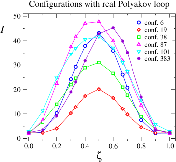
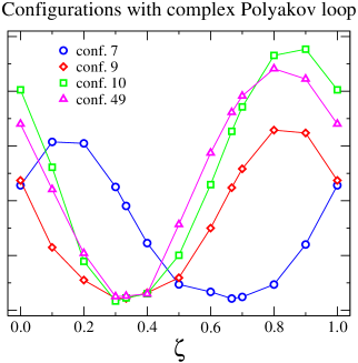
Figure 4: Inverse participation ratio $I$ as a function of $\zeta$. We show the results for the deconfined phase ($6\times 20^{3},\beta=8.45$), displaying configurations with real Polyakov loop in the l.h.s. plot and configurations with complex Polyakov loop in the r.h.s. plot.

Let us begin with looking at the behavior of the inverse participation ratio, i.e. the localization property. The discussion in the last section and the example shown there suggest that for all configurations in the real sector the inverse participation ratio has a maximum near $\zeta=0.5$ (the zero-mode is most localized there) and a minimum near $\zeta=0,1$. For configurations with complex Polyakov loop the whole curve is shifted such that the minimum is at $\zeta=1/3$ for $\varphi=2\pi/3$ and at $\zeta=2/3$ for $\varphi=-2\pi/3$. Note that this behavior is independent from a possible change of the position of the peak.

In Fig. 4 we show for all configurations in the deconfined phase where we did runs with small steps for $\zeta$ how the localization changes as a function of $\zeta$. The l.h.s. plot gives the results for configurations with real Polyakov loop, while the r.h.s. plot is for complex Polyakov loop.

The plots show that indeed for all these configurations the predicted pattern holds. The configurations with real Polyakov loop (l.h.s. plot) have a maximum of $I$ near $\zeta=0.5$ and minima near 0 and 1. For configurations with complex Polyakov loop (r.h.s. plot) we find the curve shifted such that the minimum is at $\zeta=1/3$ for phase $\varphi=2\pi/3$ (configurations 9, 10, 49 in the r.h.s. plot) and at $\zeta=2/3$ for phase $\varphi=-2\pi/3$ (configuration 7).

From the above discussions of the properties of KvB zero-modes and the examples we gave one can derive another prediction. This prediction links the distance between the positions of the lumps in the zero-mode with periodic and anti-periodic boundary conditions to the phase of the Polyakov loop: For real Polyakov loop the periodic mode with $\zeta=0$ can sit in either the interval $[0,0]$ or in the interval $[0,1]$, while the periodic zero-mode with $\zeta=0.5$ is only contained in $[0,1]$. Thus for real Polyakov loop the periodic and the anti-periodic zero-mode can be located at different positions. The situation is different for complex Polyakov loop. E.g. for $\varphi=-2\pi/3$ both $\zeta=0$ and $\zeta=0.5$ are contained in the interval $[-1/3,2/3]$ and the periodic as well as the anti-periodic zero-mode are expected to be located at the same position.

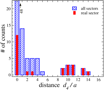
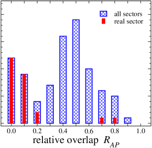
Figure 5: Histograms for the distance $R_{AP}$ between the peaks in the scalar density when comparing periodic to anti-periodic b.c. (l.h.s. plot) and for the corresponding relative overlap $R_{AP}$ (r.h.s. plot). The data are for the deconfined ensemble on $6\times 20^{3}$ lattices at $\beta=8.45$.

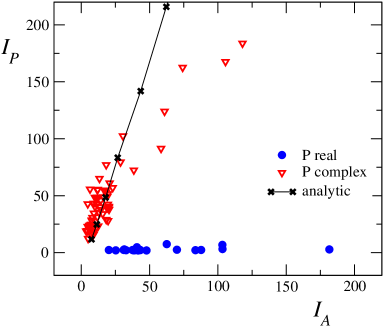
Figure 6: Scatter plot for the inverse participation ratio of the zero mode with periodic and anti-periodic boundary conditions. The data are for the deconfined ensemble on $6\times 20^{3}$ lattices at $\beta=8.45$. We use filled circles for configurations with real Polyakov loop and open triangles for the complex sector. We also include numbers (crosses connected with straight lines to guide the eye) that were generated from the analytic solution.

In Fig. 5 we test this property and in the l.h.s. plot show histograms of the distance between the peaks in the scalar density when comparing periodic to anti-periodic temporal boundary conditions. From the histogram it is obvious that indeed all configurations with large distances between the peaks, i.e. distances larger than 5 lattice spacings (0.47 fm) have real Polyakov loop. About a third of the configurations with complex Polyakov loop also show small but non-zero distances (up to distance 5 for a single configuration) between the periodic and the anti-periodic lump. We believe that this is due to quantum fluctuations superimposed on the lumps. Note that also for real Polyakov loop the KvB zero modes can sit at the same position a case which is realized by about half of the zero modes in the real sector. The plot on the r.h.s. of Fig. 5 shows histograms for the relative overlap $R_{AP}$ of the periodic and the anti-periodic zero mode. These results corroborate the findings of the histograms for the distance since the configurations which have no or only small overlap are all in the real sector. Note that a relative overlap smaller than 1 can also come from two modes which sit at the same position but have different localization. This explains why also configurations in the complex sector have relative overlap smaller than 1 (compare also Fig. 6 and the corresponding discussion below).

Finally in Fig. 6 we show a scatter plot of the values of the inverse participation ratios $I_{P},I_{A}$ for periodic and anti-periodic boundary conditions. For the real sector the mode is delocalized and $I_{P}$ is small. Thus one expects that in the $I_{P}$ versus $I_{A}$ scatter plot the data fall on a horizontal line. Our numerical results clearly show this behavior. For the complex sector the periodic mode has a scale parameter $\sigma\sim 1/3$ while the anti-periodic zero mode has $\sigma\sim 1/6$. Thus one expects $I_{P}>I_{A}$ for the complex sector and again our data nicely confirm this prediction. The plot also contains numbers of $I_{P}$ and $I_{A}$ that were generated from the analytic solution for complex Polyakov loop. We varied the positions $\vec{y}_{i}$ of the monopoles thus obtaining different values for the inverse participation ratio. These data are shown as crosses in the plot and we connect them to guide the eye. Our numerical results in the complex sector follow this analytic curve quite well. Only for very strongly localized modes ($I_{P}>100$) we see a slight deviation. We remark that on the lattice such strongly localized states are resolved by only a few lattice points such that cut-off effects become important.

4.4 Results for the spectral gap

The chiral condensate is related to the spectral density $\rho_{spec}(\lambda)$ of the Dirac operator near the origin through the Banks-Casher formula [8],

$$\langle\overline{\psi}\psi\rangle\;\;=\;\;-\,\lim_{V\rightarrow\infty}\,\frac{\pi}{V}\,\rho_{spec}(0)\;.$$ (4.26)

For the confining phase where chiral symmetry is broken the spectral density extends all the way to the origin. In the deconfined phase where chiral symmetry is restored a gap opens up in the spectral density near the origin. $\rho_{spec}(0)$ vanishes and so does the condensate. The opening up of the spectral gap is believed to come from an arrangement of instantons and anti-instantons to tightly bound molecules [5].

An interesting question is whether the chiral condensate vanishes at the same temperature for all sectors of the Polyakov loop. Results [24] for staggered fermions with anti-periodic temporal b.c. seemed to indicate that the chiral condensate vanishes at different temperatures for real and complex Polyakov loop, and attempts to understand this phenomenon can be found in [25]. A more recent study [18] analyzing directly the spectral gap (also with anti-periodic temporal b.c.) came to a different conclusion: The spectral gap appears at the same critical temperature for all sectors of the Polyakov loop and this temperature coincides with the deconfinement transition. Here we further corroborate the scenario of a single transition by discussing the spectral gap for different boundary conditions for the Dirac operator.

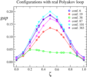
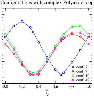
Figure 7: Size of the spectral gap as a function of $\zeta$. We show the results for the deconfined phase, displaying configurations with real Polyakov loop in the l.h.s. plot and configurations with complex Polyakov loop in the r.h.s. plot.

In Fig. 7 we show the spectral gap as a function of the boundary condition parameter $\zeta$ for the 10 configurations in the deconfined phase where spectra with finely spaced $\zeta$ were computed. The l.h.s. plot shows the 6 configurations with real Polyakov loop, while the r.h.s plot gives data for the configurations with complex Polyakov loop. The spectral gap is defined as the size of the imaginary part of the smallest complex eigenvalue.

The plots show that as for the inverse participation ratio the results for the gap from configurations with $\varphi=\pm 2\pi/3$ for the Polyakov loop can be obtained from the result for $\varphi=0$ by shifting the $\zeta$ axis by amounts of $1/3$ and $2/3$ respectively. The results in the three sectors are completely equivalent (with only the data for configuration 38 showing a somewhat irregular behavior) and can be transformed into each other through different boundary conditions for the fermions. This symmetry shows that there is no reason to expect a different critical temperature for chiral symmetry restoration in different sectors of the Polyakov loop.

It is interesting to note that in the real sector for $\zeta=0$ and in the complex sectors for $\zeta=1/3$, respectively $\zeta=2/3$ the spectral gap becomes very small. This could indicate that for these boundary conditions chiral symmetry remains broken also in the deconfined phase. It would be interesting to analyze the chiral condensate in the deconfined phase using these boundary conditions for the fermions.

5 Finite Temperature - results below $T_{c}$

5.1 Overview over the configurations

In the last section we have studied the behavior of the configurations in the deconfined phase. We have found that qualitatively our results match the characteristics of the KvB solutions very well. In this section we now turn to the ensemble below $T_{c}$. Below $T_{c}$ the Polyakov loop vanishes which leaves only the unique possibility,

$$(\mu_{1},\mu_{2},\mu_{3},\mu_{4})\;\;=\;\;(-1/3,0,1/3,2/3)\;,$$ (5.27)

for the phase factors $\mu_{i}$. One expects that the zero-modes can change their position when $\zeta$ crosses the values of $1/3$ and $2/3$. Thus below $T_{c}$ the zero-mode can change its position more often and for these configurations we now use a finer spacing of $\zeta$.

conf.	$I_{P}$	$I_{A}$	$(t,x,y,z)^{max}_{P}$				$(t,x,y,z)^{max}_{A}$				$d_{4}/a$	# lumps
13	4.67	13.41	5	11	16	11	2	1	9	6	13.52	4
18	7.32	10.73	2	6	20	3	6	16	15	12	14.49	3
92	38.52	5.73	1	11	13	13	4	8	16	11	5.56	2
109	5.56	15.93	1	14	18	18	2	18	5	3	9.53	4
123	4.59	32.21	5	18	19	11	4	13	18	1	11.26	2
125	4.13	14.72	5	1	16	9	5	14	16	18	11.40	3
153	22.98	10.32	5	17	18	19	6	18	17	2	3.46	2
210	2.48	28.96	1	1	8	4	2	2	1	13	11.48	3
215	7.23	3.63	1	15	20	14	5	11	17	6	9.64	3
266	8.15	40.01	1	9	19	20	2	9	6	6	9.27	3

Table 4: Parameters of the subensemble below $T_{c}$ ($6\times 20^{3},\beta=8.20$) which we studied with finely spaced values for the boundary parameter $\zeta$. For these 10 configurations we list the configuration number, the inverse participation ratios $I_{P}$ and $I_{A}$ for the zero-modes with periodic, respectively anti-periodic b.c., the position of the maxima for the corresponding zero-modes, the 4-distance $d_{4}$ between these two maxima and the number of different lumps visited by the mode in a complete cycle through $\zeta$.

From the complete ensemble below $T_{c}$ (compare Table 1) we computed for 10 configurations eigenvectors at all values of $\zeta$ between $\zeta=0$ and $\zeta=1$ in steps of 0.05. In Table 4 we list some basic properties of these configurations. In particular we list the configuration number, the inverse participation ratios $I_{P}$ and $I_{A}$ for the zero-modes with periodic, respectively anti-periodic b.c., the position of the maxima for the corresponding zero-modes and the 4-distance $d_{4}$ between these two maxima in lattice units. Finally we list the number of different lumps visited by the mode in a complete cycle through $\zeta$. We count a lump as independent lump when its maximum remains at the same position for at least 3 subsequent values of $\zeta$, i.e. dominates the zero mode at least for a $\zeta$-interval of length 0.1. Note that these lumps are visited by the zero-mode one after the other and typically one of them dominates the zero-mode.

A first interesting finding can already be read off from the numbers in the table. As discussed, below $T_{c}$ the zero mode has three possible values of $\zeta$ where it can change position, $\zeta=0,1/3,2/3$. Thus the zero-mode can visit up to 3 different positions. Also a number less than 3 is possible since the coordinate vectors $\vec{y}_{i}$ of the monopoles can coincide. Most of the eigenmodes do indeed see 2 or 3 lumps but for two of the configurations (13 and 109) we found 4 lumps. This observation indicates that for our ensemble below $T_{c}$ the zero-modes do not follow the predictions for KvB zero-modes as closely as their counterparts above $T_{c}$. Reasons for that may be quantum effects which drive the trace of the Polyakov loop away from zero. We also remark that the lattice below $T_{c}$ is coarser than the lattice above $T_{c}$.

5.2 Example for the generic behavior

As for the ensemble in the deconfined phase we begin the presentation of our results with showing slices of the scalar density for a generic example. As discussed in the last subsection, below $T_{c}$ the zero-mode is expected to visit up to three different lumps in a complete cycle through the boundary condition. Configuration 125 is an example for such a behavior. In Table 5 we list some basic properties of this configuration for all values of $\zeta$ we studied.

$\;\;\zeta$	$I$	$(t,x,y,z)^{max}$				$\;\;\zeta$	$I$	$(t,x,y,z)^{max}$
0.0	4.13	5	13	6	9	0.55	16.61	5	6	6	18
0.05	5.70	5	13	6	9	0.6	18.36	5	6	6	18
0.1	6.03	5	6	6	18	0.65	18.07	5	6	6	18
0.15	6.26	5	6	6	18	0.7	16.17	5	6	6	18
0.2	5.50	2	6	13	19	0.75	13.10	5	6	6	18
0.25	5.60	2	6	13	19	0.8	8.71	5	6	6	18
0.3	6.18	2	6	13	19	0.85	4.81	5	6	6	18
0.35	8.98	2	6	13	19	0.9	4.16	5	13	6	9
0.4	12.60	5	6	6	18	0.95	4.18	5	13	6	9
0.45	14.21	5	6	6	18	1.0	4.13	5	13	6	9
0.5	14.72	5	6	6	18

Table 5: Inverse participation ratio and position of the maximum of the scalar density as a function of the boundary condition parameter $\zeta$. The data are for configuration 125 of the confined ensemble ($6\times 20^{3},\beta=8.20$).

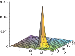
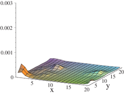
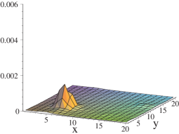
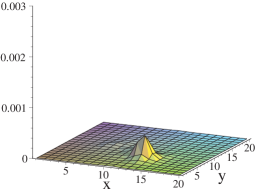
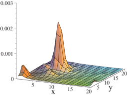
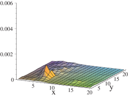
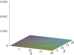
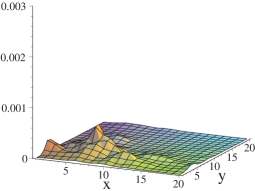
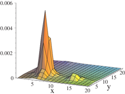
Figure 8: Slices of the scalar density for $6\times 20^{3},\beta=8.20$, configuration 125. We show $x,y$-slices at $t=5$, $z=9$ (left column), at $t=2$, $z=19$ (center column) and $t=5$, $z=18$ (right column). The values for $\zeta$ are $\zeta=0.05,0.3,0.65$ (from top to bottom).

Table 5 shows that the zero-mode of configuration 125 visits three different lumps located at $(t,x,y,z)$ = (5,13,6,9), (2,6,13,19) and (5,6,6,18). These three lumps are well separated from each other with mutual 4-distances of $d_{4}=14.38$, $d_{4}=11.40$ and $d_{4}=7.68$ in units of the lattice spacing. In fermi this is $d_{4}=$ 1.65 fm, 1.31 fm and 0.88 fm. The most prominent lump is the one at $(t,x,y,z)=(5,6,6,18)$ which is seen by the zero mode at all $\zeta$ between $\zeta=0.4$ and $\zeta=0.85$. We remark that this lump is also the most localized one, i.e. reaches the largest values for the inverse participation ratio. This is as expected for the KvB zero-modes, where the mass of the underlying monopole is proportional to $\mu_{m+1}-\mu_{m}$ (compare Eq. 3.15). Thus the lump which occupies the largest interval in $\zeta$ is also the most localized one. This pattern also holds for all other configurations listed in Table 4. It is interesting to note that the lump at $(t,x,y,z)=(5,6,6,18)$ already briefly appears at $\zeta=0.1,0.15$ before the lump at $(t,x,y,z)=(2,6,13,19)$ takes over. The reason for that is that the lump at (2,6,13,19) starts to grow only slowly such that for the small window in $\zeta$ the remains of the tallest lump at (5,6,6,18) dominate.

Let us now look at plots for the scalar density for this configuration. In Fig. 8 we show $x,y$-slices for the scalar density taken through the maxima of the three lumps, i.e. at $t=5$, $z=9$ (left column), at $t=2$, $z=19$ (center column) and $t=5$, $z=18$ (right column). The values for $\zeta$ are $\zeta=0.05,0.3,0.65$. These are the values where the dominating lumps have their maximum. In between these extremal values one has intermediate situations with a receding and an advancing lump. Note that the plots in the r.h.s. column have a different scale and the corresponding lump is about twice as tall as the other two lumps.

It is interesting to inspect also other slices, in particular a slice containing the time direction. For an unperturbed KvB solution one expects that the lump extends over all of the time direction and that the height of the lump displays an oscillating behavior in time. For the action density of cooled SU(2) lattice configurations with twisted boundary conditions such a behavior was observed in [11].

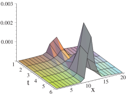
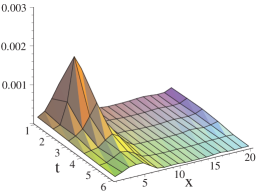
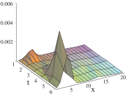
Figure 9: Slices of the scalar density for $6\times 20^{3},\beta=8.20$, configuration 125. We show $t,x$-slices at $y=6$, $z=9$ for $\zeta=0.05$ (left plot), at $y=13$, $z=19$ for $\zeta=0.3$ (center plot) and $y=6$, $z=18$ for $\zeta=0.65$ (right plot). These plots correspond to the three dominant lumps also shown in Figs. 8.

In Fig. 9 we show $t,x$-slices of the scalar density again for configuration 125 which was already used for the plots in Fig. 8. In particular we show the slices through the 3 lumps at their dominant value of $\zeta$. They were taken at $y=6$, $z=9$ for $\zeta=0.05$ (left column), at $y=13$, $z=19$ for $\zeta=0.3$ (center column) and $y=6$, $z=18$ for $\zeta=0.65$ (right column). The plots show that all three lumps are stretched along the $t$-axis. A similar behavior was also observed for other configurations, both below and above $T_{c}$.

5.3 Results from the whole sample

As for the deconfined phase, also for the ensemble below $T_{c}$ we now study observables evaluated for the whole ensemble in order to establish properties of the zero-modes beyond a demonstration in a single example.

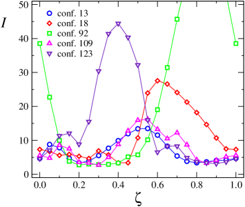
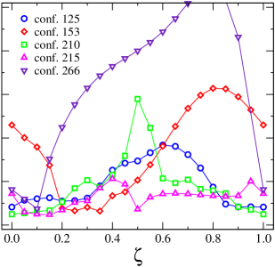
Figure 10: Inverse participation ratio $I$ as a function of $\zeta$ for the $6\times 20^{3}$, $\beta=8.20$ ensemble. In order to avoid overcrowded figures we show the data for configurations 13, 18, 92, 109 and 123 on the l.h.s., and configurations 125, 153, 210, 215, 266 on the r.h.s.

We start with plots for the inverse participation ratio as a function of $\zeta$. In Fig. 10 we show such figures for the 10 configurations with finely spaced $\zeta$ listed in Table 4. To avoid overcrowding of the plots we split the figure into two plots and show the data for configurations 13, 18, 92, 109 and 123 on the l.h.s., and configurations 125, 153, 210, 215, 266 on the r.h.s.

From the plots it is obvious that the localization of the zero-mode fluctuates strongly during a complete cycle through the boundary condition. Typically there is a single pronounced maximum in the inverse participation ratio and one or two local maxima. The tallest peak occupies also the largest interval of $\zeta$ in accordance with the mass formula Eq. (3.15). On the other hand it is obvious from the plots that the minima are not necessarily located at exactly $\zeta=0$, $\zeta=1/3$ and $\zeta=2/3$ as would be the case for an unperturbed KvB zero-mode. However, one should not forget that our configurations are taken from a thermalized ensemble containing all quantum effects. It is not yet known [26] in which way quantum effects modify the classical KvB solutions.

In Fig. 11 we show histograms for the distance $d_{4}$ between the lump in the periodic and anti-periodic zero-modes in the l.h.s. plot. On the r.h.s. we show a histogram for the relative overlap $R_{AP}$ between these two lumps. These two histograms contain the data for all 70 configurations in the ensemble.

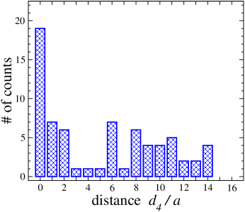
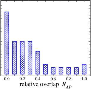
Figure 11: Histograms for the distance $d_{4}$ between the peaks in the scalar density when comparing periodic to anti-periodic b.c. (l.h.s. plot) and for the relative overlap $R_{AP}$ between the two zero-modes (r.h.s. plot). The data are for the ensemble in the confining phase on $6\times 20^{3}$ lattices at $\beta=8.20$.

The histogram on the l.h.s. shows that for half of the configurations the zero-mode for periodic boundary conditions and its anti-periodic counterpart sit on lumps which are more than 5 lattice spacings apart, i.e. at least 0.69 fm. The plot on the r.h.s. supports this finding by illustrating that typically the two lumps do not overlap substantially. Note that even if the lumps are located at the same position their relative overlap can be smaller than 1 when they differ in size. Both plots in Fig. 11 show that configurations where the zero-mode changes its location and size are not singular events but make up a large portion of the ensemble.

6 Results on the torus

6.1 Overview over the configurations

Having successfully identified the substructure predicted for the KvB zero-modes in ensembles with high temperature it is natural to apply the same techniques to configurations at low temperature. In this section we perform such an exploratory study and analyze our ensemble on $16^{4}$ lattices with $\beta=8.45$. The difference to the high temperature configurations is that the lattice geometry does not single out a time direction. We break the euclidean symmetry explicitly and use our generalized fermionic boundary condition for the 1-direction, while for the other directions we implement periodic boundary conditions. We remark that on the torus no analytic results are available to compare with.

As for the cases with temperature we compute eigenvectors of the Dirac operator with different values of the boundary condition parameter $\zeta$. For all 46 configurations of the ensemble (compare Table 1) we use $\zeta=0$ and $\zeta=0.5$, i.e. periodic and anti-periodic boundary conditions. For a subensemble of 10 configurations we computed eigenvectors for all values of $\zeta$ between 0 and 1 in steps of 0.1.

conf.	$I_{P}$	$I_{A}$	$(t,x,y,z)^{max}_{P}$				$(t,x,y,z)^{max}_{A}$				$d_{4}/a$	# lumps
32	6.84	8.62	5	9	5	8	15	5	8	15	10.48	2
61	51.85	66.22	14	11	8	7	14	11	8	7	0.00	1
64	3.08	3.43	11	12	13	2	7	2	12	5	7.87	3
82	3.96	3.98	3	15	5	5	4	1	15	2	7.07	2
93	2.47	3.00	3	7	5	14	8	11	4	6	10.29	3
103	2.54	3.04	4	14	3	2	4	14	3	2	0.00	1
351	3.06	3.73	14	10	3	7	7	4	6	12	10.90	3
354	7.67	11.86	13	14	4	4	13	14	4	4	0.00	1
522	7.32	2.71	3	14	16	6	16	11	15	7	4.47	3
561	3.94	6.74	8	3	15	8	14	4	9	9	8.60	1

Table 6: Parameters of our ensemble on the torus ($16^{4},\beta=8.45$). We list the configuration number, the inverse participation ratios $I_{P}$ and $I_{A}$ for the zero-modes with periodic, respectively anti-periodic b.c., the position of the maxima for the corresponding zero-modes, the 4-distance $d_{4}$ between these two maxima and the number of different lumps visited by the mode in a complete cycle of $\zeta$.

For these 10 configurations Table 6 shows some basic properties. In particular we list the configuration number, the inverse participation ratio for the periodic and anti-periodic zero-modes, the positions of the maxima in the corresponding scalar densities and the difference between these two peaks. In addition we display the number of lumps visited by the zero-mode in a complete cycle through the phase at the boundary. Here we count a lump as independent if it appears at two subsequent values of $\zeta$, i.e. is visible in a $\zeta$-interval of at least length 0.1. This is the same criterion used for the $6\times 20^{3},\beta=8.20$ ensemble.

The table makes obvious that also for the ensemble on the torus we do find configurations where the zero-mode is located at different positions for different values of $\zeta$. The 4-distances between the periodic and the anti-periodic lumps reach values up to 11 in lattice units which is up to 1.03 fm. When discussing the complete ensemble we will find that about half of the configurations have a sizeable distance between the two peaks. The zero-modes visit between 1 and 3 different lumps in a complete cycle of $\zeta$. We remark that although for configuration 561 we have $d_{4}\neq 0$ we list only a single lump in the last column. The reason is that only for $\zeta=0$ the zero-mode is located at a different position and thus the criterion of two subsequent appearances is not fulfilled. The pattern observed for this configuration is similar to the pattern of a configuration in the deconfined phase with real Polyakov loop.

6.2 Example for the generic behavior

Let us now look at figures of the scalar density for a typical configuration. In particular we will show plots for configuration 32 of our ensemble. Before presenting these figures we discuss Table 7 where we list some properties of this configuration as a function of $\zeta$. In the left half of the table we show $\zeta$, the inverse participation ratio and the position of the maximum. The zero-mode changes its position at $\zeta=0.3$ and $\zeta=0.9$. The localization shows some mild changes with reaching local maxima at $\zeta=0.5$ and $\zeta=0.1$, i.e. approximately in the middle of the $\zeta$-intervals for the two lumps.

In the right half of the table we show the data from a small consistency check which we performed for 4 of the 10 configurations. We switched the direction where we apply the boundary condition from the 1-direction to the 2-direction. Since our lattice does not single out a particular direction any direction for applying the boundary condition serves equally well and the results should be consistent. The data in the right half of the table show that this is indeed the case. Also with the non-trivial boundary condition applied in the 2-direction we see the same two lumps at (5,9,5,8) and (15,5,8,15). They appear, however, at different values of $\zeta$ which is not surprising since a single gauge configuration does not respect rotational symmetry. Also for the other 3 configurations where we experimented with changing the direction we single out by the boundary condition, we find that essentially the same lumps are seen, again at slightly different values of $\zeta$.

b.c. in 1-direction:						b.c. in 2-direction:
$\;\;\zeta$	$I$	$(t,x,y,z)^{max}$				$\;\;\zeta$	$I$	$(t,x,y,z)^{max}$
0.0	6.84	5	9	5	8	0.0	6.84	5	9	5	8
0.1	7.47	5	9	5	8	0.1	6.01	5	9	5	8
0.2	7.09	5	9	5	8	0.2	4.54	15	5	8	15
0.3	6.86	15	5	8	15	0.3	9.76	15	5	8	15
0.4	7.56	15	5	8	15	0.4	8.44	15	5	8	15
0.5	8.62	15	5	8	15	0.5	5.73	15	5	8	15
0.6	7.50	15	5	8	15	0.6	4.97	15	5	8	15
0.7	5.22	15	5	8	15	0.7	5.11	5	9	5	8
0.8	3.91	15	5	8	15	0.8	5.71	5	9	5	8
0.9	4.87	5	9	5	8	0.9	6.49	5	9	5	8
1.0	6.84	5	9	5	8	1.0	6.84	5	9	5	8

Table 7: Inverse participation ratio and position of the maximum of the scalar density as a function of the boundary condition parameter $\zeta$. The data are for configuration 32 of the ensemble on the torus ($16^{4},\beta=8.45$). The data in the left half of the table were obtained with using the nontrivial boundary condition in 1-direction, while the data in the right half is for 2-direction. The corresponding plots of the scalar density are shown in Fig. 12.

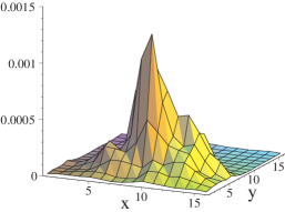
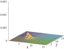
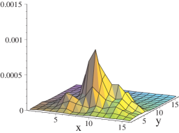
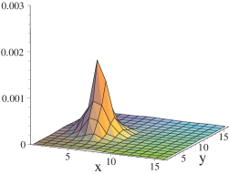
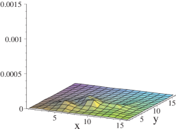
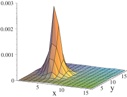
Figure 12: Slices of the scalar density for $16^{4},\beta=8.45$, configuration 32. We show $x_{2},x_{3}$-slices (in the plots we again label these two axes as $x$ and $y$) at $x_{1}=5$, $x_{4}=8$ (left column) and at $x_{1}=15$, $x_{4}=15$ (right column). The values for $\zeta$ are (from top to bottom) $\zeta=0,0.3,0.5$. Note the different scale for the l.h.s. and r.h.s. plots.

In Fig. 12 we show $x_{2},x_{3}$-slices of the scalar density for configuration 32 (in the plots we again label these two axes as $x$ and $y$). The slices were taken through the maxima of the two peaks, i.e. at $x_{1},x_{4}$ = 5,8 (left column of plots), respectively at $x_{1},x_{4}$ = 15,15 (right column of plots). We use values of $\zeta=0,0.3,0.5$ showing the two extremal situations where only one of the lumps dominates ($\zeta=0$, top) and $\zeta=0.5$, bottom) and an intermediate situation ($\zeta=0.3$, middle). Note the different scale for the two columns of plots. The data we show are from the run with the boundary phase attached in 1-direction. The plots show clearly that the zero-mode changes its location with $\zeta$. The same pattern with certain values of $\zeta$ where a single lump dominates and intermediate values with an advancing and a retreating lump is also seen for the other configurations which visit two or three lumps. Equivalent plots taken for the zero-modes computed with boundary conditions in 2-direction show similar behavior. The lumps sit at the same positions and even have similar shape, such as e.g. the slightly elongated form along the $x$-axis in the plots in the left columns.

6.3 Results from the whole sample

Let us now try to analyze the common features of all configurations in the ensemble. We start with discussing the inverse participation ratio as a function of $\zeta$. In Fig. 13 we show two such figures where we again distribute the 10 configurations among two plots, with the l.h.s. plot containing configurations 32, 64, 82 and 93 and configurations 103, 351, 354, 522, 561 on the r.h.s. We remark that configuration 61 which is also listed in Table 6 has values of $I$ above 50 for all $\zeta$ such that this defect-like lump does not show up for the plot-range we have chosen.

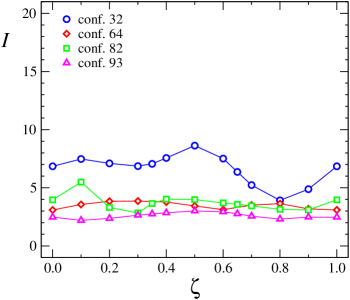
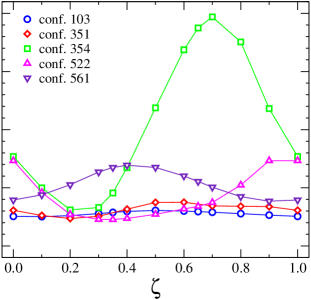
Figure 13: Inverse participation ratio $I$ as a function of $\zeta$ for the $16^{4}$, $\beta=8.45$ ensemble. In order to avoid overcrowded figures we show the data for configurations 32, 64, 82 and 93 on the l.h.s., and configurations 103, 351, 354, 522, 561 on the r.h.s.

The plots show that some of the configurations display quite a sizeable change in their localization as a function of $\zeta$. Four of the zero-modes (64, 93, 103, 351) show only relatively small changes of their inverse participation ratio. An inspection of Table 6 shows that this behavior seems to be correlated with neither $d_{4}$ nor with the number of lumps visited by the zero-mode.

Let us now address the question whether changing its location is a common property of the zero-modes for our ensemble on the torus. We do this by again analyzing histograms for the distance $d_{4}$ between the maxima of the periodic and anti-periodic scalar density and histograms for the overlap between the two lumps. In Fig. 14 we show such plots with the histogram for the distance on the l.h.s. and the histogram for the overlap on the r.h.s. The histograms were taken from all 46 configurations in our ensemble on the torus.

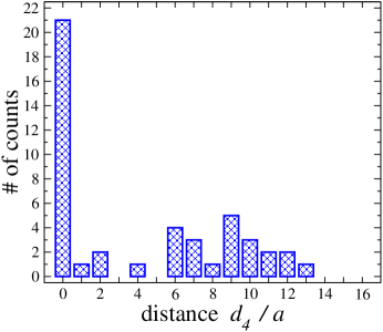
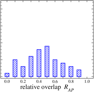
Figure 14: Histograms for the distance between the peaks in the scalar density when comparing periodic to anti-periodic b.c. (l.h.s. plot) and for the relative overlap (r.h.s. plot). The data are for the ensemble on the torus ($16^{4}$, $\beta=8.45$).

The histogram for the distance $d_{4}$ shows that indeed configurations are quite abundant where the zero-mode changes its position by a sizeable amount, larger than a simple deformation by a fluctuation. In particular about half of the configurations show a $d_{4}$ of at least 6 in lattice units, i.e. the centers of the lumps are at least 0.56 fm apart. The distance $d_{4}$ reaches values up to 13 in lattice units, i.e. 1.22 fm. The histogram for the relative overlap shows that even most of the zero-modes that do not change their location suffer some deformation when changing the boundary condition, such that the relative overlap is pushed below 1.

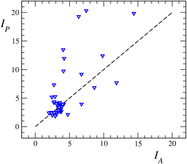
Figure 15: Scatter plot for the inverse participation ratio of the zero mode with periodic and anti-periodic boundary condition ($I_{P}$ respectively $I_{A}$). The data (triangles) are for the ensemble on the torus ($16^{4}$, $\beta=8.45$). We display the line with $I_{P}=I_{A}$ as a dashed line.

Finally in Fig. 15 we show a scatter plot of the periodic inverse participation ratio $I_{P}$ versus its anti-periodic counterpart $I_{A}$. For the deconfined phase the equivalent plot shown in Fig. 6 has revealed an asymmetry between periodic and anti-periodic boundary conditions which is closely related to the critical values of $\zeta$ where the zero-mode can change its location. For the ensemble on the torus our Fig. 15 does not reveal such a structure and the data essentially scatter symmetrically around the line $I_{P}=I_{A}$ which we display as a dashed straight line. This indicates that for the torus we do not find a pronounced pattern which links the localization of the mode to particular values of $\zeta$.

7 Summary

In this article we have studied properties of topological excitations of SU(3) lattice gauge configurations with topological charge $Q=\pm 1$. Through the index theorem such configurations give rise to a single zero-mode of the Dirac operator. The zero-mode is localized on the topological excitation and reflects the properties of the underlying lump in the gauge field. We analyzed how the zero-mode changes when applying an arbitrary phase $\exp(i2\pi\zeta)$ at the temporal boundary condition for the Dirac operator. Our main findings are:

• For the ensemble in the deconfined phase we find that the zero-mode can change its position at $\zeta=0$ for configurations with real Polyakov loop and at $\zeta=1/3,\zeta=2/3$ for configurations in the complex sector.

• The zero-mode is very spread out at these critical values and most localized for $\zeta=0.5$ for real Polyakov loop, respectively $\zeta=5/6,\zeta=1/6$ for the complex sectors.

• These observations nicely match the predictions for zero-modes of KvB solutions.

• An analysis of the spectral gap shows the same periodic behavior in $\zeta$ supporting earlier findings of only a single transition temperature for chiral symmetry restoration in all sectors of the Polyakov loop.

• For the ensemble in the confined phase just below $T_{c}$ we find that for a large portion of our ensemble the zero-mode is located at different positions when changing the boundary condition.

• Also the localization of the mode fluctuates considerably during a complete cycle through $\zeta$.

• When analyzing the time dependence one finds that the zero-modes are stretched along the time direction for both ensembles above and below $T_{c}$.

• Several properties of zero-modes in the confined phase match predictions for KvB zero modes, but the resemblance is not as close as in the deconfined phase.

• Also the zero-modes for configurations on the torus change their location when changing the phase at the boundary.

• The results obtained when applying the boundary condition at different directions are consistent with each other.

• About half of our torus configurations have zero-modes located at different positions when comparing periodic to anti-periodic boundary conditions.

Our results show that for a large portion of our configurations an excitation with topological charge $|Q|$ = 1 is not a single lump. Instead it is built from several independent objects and does not resemble a simply connected instanton-like object.

Acknowldegements:
We thank Meinulf Göckeler, Michael Müller-Preussker, Paul Rakow, Andreas Schäfer and Christian Weiss for discussions. We are particularly greatful for the ongoing interest from Pierre van Baal who generously shared his insight and experience with us. Christof Gattringer thanks the Austrian Academy of Science for support (APART 654). This project was partly supported by BMBF and DFG. The calculations were done on the Hitachi SR8000 at the Leibniz Rechenzentrum in Munich and we thank the LRZ staff for training and support.

References

-
[1]
T.L. Ivanenko and J.W. Negele,
Nucl. Phys. Proc. Suppl. 63 (1998) 504;
M. Göckeler, P.E.L. Rakow, A. Schäfer, W. Söldner, T. Wettig, Phys. Rev. Lett. 87 (2001) 042001; T. DeGrand, Phys. Rev. D 64 (2001) 094508. - [2] I. Horváth, N. Isgur, J. McCune and H.B. Thacker, Phys. Rev. D 65 (2002) 014502; T. DeGrand and A. Hasenfratz, Phys. Rev. D 65 (2002) 014503; T. Blum et al., Phys. Rev. D 65 (2002) 014504; R.G. Edwards and U.M. Heller, Phys. Rev. D 65 (2002) 014505; I. Hip, T. Lippert, H. Neff, K. Schilling and W. Schroers, Phys. Rev. D 65 (2002) 014506; C. Gattringer, M. Göckeler, P.E.L. Rakow, S. Schaefer, A. Schäfer, Nucl. Phys. B 617 (2001) 101, Nucl. Phys. B 618 (2001) 205, P. Hasenfratz, S. Hauswirth, K. Holland, T. Jörg and F. Niedermayer, Nucl. Phys. Proc. Suppl. 106 (2002) 751.
- [3] C. Gattringer, Phys. Rev. Lett. 88 (2002) 221601.
- [4] I. Horváth et al., Phys. Rev. D 66 (2002) 034501.
- [5] D. Diakonov and V.Y. Petrov, Phys. Lett. B 147 (1984) 351; Nucl. Phys. B 272 (1986) 457; D. Diakonov, hep-ph/0212026, and references therein; T. Schäfer and E.V. Shuryak, Rev. Mod. Phys. 70 (1998) 323 and references therein.
- [6] M. Atiyah and I.M. Singer, Ann. Math. 87 (1968) 596, Ann. Math. 93 (1971) 139.
- [7] G. ’t Hooft, Phys. Rev. D 14 (1976) 3432.
- [8] T. Banks and A. Casher, Nucl. Phys. B169 (1980) 103.
- [9] T.C. Kraan and P. van Baal, Phys. Lett. B 428 (1998) 268, Nucl. Phys. B 533 (1998) 627, Phys. Lett. B 435 (1998) 389; F. Bruckmann and P. van Baal, Nucl. Phys. B 645 (2002) 105.
- [10] B.J. Harrington and H.K. Shepard, Phys. Rev. D 17 (1978) 2122, Phys. Rev. D 18 (1978) 2990.
- [11] M. Garcia Pérez, A. González-Arroyo, A. Montero and P. van Baal, JHEP 9906 (1999) 001.
- [12] E.M. Ilgenfritz, B.V. Martemyanov, M. Müller-Preussker, S. Shcheredin and A.I. Veselov, Phys. Rev. D 66 (2002) 074503, hep-lat/0209081.
- [13] M. Garcia Pérez, A. González-Arroyo, C. Pena and P. van Baal, Phys. Rev. D 60 (1999) 031901; M.N. Chernodub, T.C. Kraan and P. van Baal, Nucl. Phys. Proc. Suppl. 83 (2000) 556.
- [14] C. Gattringer, Phys. Rev. D 67 (2003) (in print), hep-lat/0210001.
- [15] C. Callan, R. Dashen and D. Gross, Phys. Rev. D 17 (1978) 2717; A. González-Arroyo and P. Martinez, Nucl. Phys. B 459 (1996) 337; A. González-Arroyo, P. Martinez and A. Montero, Phys. Lett. B 359 (1995) 159; A. González-Arroyo and A. Montero, Phys. Lett. B 387 (1996) 823; S. Jaimungal and A. R. Zhitnitsky, hep-ph/9904377, hep-ph/9905540; J. V. Steele and J. W. Negele, Phys. Rev. Lett. 85 (2000) 4207.
- [16] M. Lüscher and P. Weisz, Commun. Math. Phys. 97 (1985) 59; Err.: 98 (1985) 433; G. Curci, P. Menotti and G. Paffuti, Phys. Lett. B 130 (1983) 205, Err.: B 135 (1984) 516.
- [17] C. Gattringer, R. Hoffmann and S. Schaefer, Phys. Rev. D 65 (2002) 094503.
- [18] C. Gattringer, P.E.L. Rakow, A. Schäfer and W. Söldner, Phys. Rev. D 66 (2002) 054502.
- [19] C. Gattringer, Phys. Rev. D 63 (2001) 114501; C. Gattringer, I. Hip, C.B. Lang, Nucl. Phys. B 597 (2001) 451; C. Gattringer and I. Hip, Phys. Lett. B 480 (2000) 112.
- [20] P. Ginsparg, K.G. Wilson, Phys. Rev. D 25 (1982) 2649.
- [21] C. Gattringer, Nucl. Phys. Proc. Suppl. (in print), hep-lat/0208056; C. Gattringer et al. [Bern-Graz-Regensburg Collaboration], Nucl. Phys. Proc. Suppl. (in print), hep-lat/0209099.
- [22] C. Gattringer, M. Göckeler, C.B. Lang, P.E.L. Rakow and A. Schäfer, Phys. Lett. B 522 (2001) 194; C. Gattringer and C.B. Lang, Comput. Phys. Commun. 147 (2002) 398.
- [23] D.C. Sorensen, SIAM J. Matrix Anal. Appl. 13 (1992) 357.
- [24] S. Chandrasekharan and N.H. Christ, Nucl. Phys. Proc. Suppl. 47 (1996) 527.
- [25] P.N. Meisinger and M.C. Ogilvie, Phys. Lett. B 379 (1996) 163; S. Chandrasekharan and S. Huang, Phys. Rev. D 53 (1996) 5100; M.A. Stephanov, Phys. Lett. B 375 (1996) 249.
- [26] P. van Baal, private communication.