Lattice calculation of the lowest order hadronic contribution to the muon anomalous magnetic moment
Abstract
We present a quenched lattice calculation of the lowest order () hadronic contribution to the anomalous magnetic moment of the muon which arises from the hadronic vacuum polarization. A general method is presented for computing entirely in Euclidean space, obviating the need for the usual dispersive treatment which relies on experimental data for annihilation to hadrons. While the result is not yet of comparable precision to those state-of-the-art calculations, systematic improvement of the quenched lattice computation to this level is straightforward and well within the reach of present computers. Including the effects of dynamical quarks is conceptually trivial, the computer resources required are not.
pacs:
12.38.Gc, 13.40.Em, 14.60.Ef, 14.65.BtThe magnetic moment of the muon is defined by the (static) limit of the vertex function which describes the interaction of the electrically charged muon with the photon,
| (1) |
where is the muon mass, is the photon momentum, and are the incoming and outgoing momentum of the muon. Lorentz invariance and current conservation have been used in obtaining Eq. 1. Form factors and contain all information about the muon’s interaction with the electromagnetic field. In particular, is the electric charge of the muon in units of , and is the Landé g-factor, proportional to the magnetic moment. The anomaly, defined as half of the difference of from its tree level value, which the Dirac equation predicts to be 2 for an elementary spin 1/2 particle, is . Thus, at tree level, and corrections to , and therefore , start at in QED where is the fine structure constant. to all orders due to charge conservation.
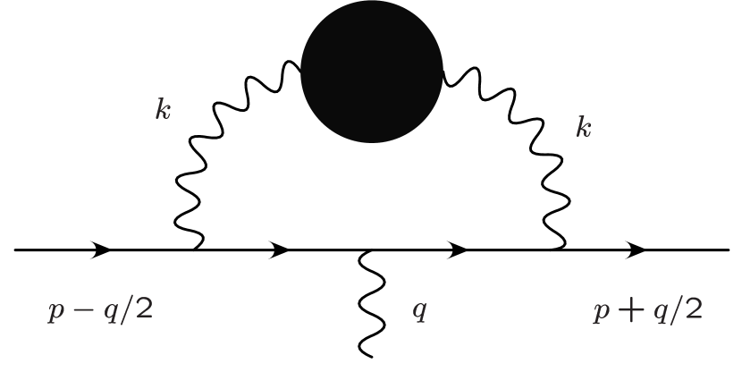
The most precise measurement ever of the muon’s anomalous magnetic moment was recently carried out at Brookhaven National LaboratoryBennett:2002jb . In Davier:2002dy ; Hagiwara:2002ma the authors quote three standard deviation discrepancies between the Standard Model and experimentBennett:2002jb . The theoretical and experimental uncertainties are roughly the same and were added in quadrature. The dominant theoretical uncertainty resides in hadronic loop corrections arising from the hadronic vacuum polarization () (see Figure 6) and hadronic light-by-light scattering (), and it is clearly of interest to reduce these errors. Presently, the hadronic contribution is calculated by using a dispersion relation and the experimental value of the total cross-section for annihilation to hadrons to relate the imaginary part of the vacuum polarization to the real part. This calculation is very precise, though a discrepancy with a calculation that uses decay data may indicate a theory error as large as five percentDavier:2002dy and reduces the disagreement with experiment to roughly 1.6 standard deviations. A purely theoretical, first principles, calculation has been lacking and is desirable, and also has several advantages over the conventional approach. For instance, the separation of QED effects from hadronic corrections is automatic, as is the treatment of isospin corrections if different quark masses are used in the simulation. Thus it is possible that lattice calculations may eventually help to settle the above mentioned discrepancy between annihilation and decay.
The method described here is simple and direct. We begin with Ref. Roskies:1990ki which describes the computation of multi-loop graphs in perturbation theory through the expansion of the integrand in terms of hyperspherical polynomials. The key is that the entire integral, including external momenta, can be Wick-rotated into Euclidean space and the angular integrals done so that what is left is an integral over the magnitude of the loop momentum. If the graph can be set up in a certain way, then after the external momenta are analytically continued on-shell, the integral over the loop momenta is performed without distorting the integration contour: , the squared Euclidean loop momentum. For the case at hand, this means the photon propagator can only depend on the loop momentum. This is important because if the photon propagator depends only on , then so will the vacuum polarization. Thus, the renormalized hadronic vacuum polarization function, calculated on the lattice and in Euclidean space, can be directly inserted into the one-loop diagram for the anomalous magnetic moment without analytically continuing the vacuum polarization back to Minkowski space, or requiring its value in a region not accessible to lattice calculations, namely . The condition on the photon propagator is easily met in this case as can be seen from the assignment of momenta in Figure 6.
Following Roskies:1990ki ; Barbieri:1972as , to extract from Eq. 1, apply a projection operator and compute . Omitting the quark loop for the moment, applying the Feynman rules, and taking the limit , the diagram in Figure 6 gives111It is well known that is neither infrared nor ultraviolet divergent; thus we use the unregularized photon propagator for simplicity.
| (2) |
where . Analytically continuing the entire amplitude to Euclidean space, including the external momenta, performing the angular integrations, and then analytically continuing back on-shell, we are left with
| (3) |
where . One can easily verify that this gives the leading Schwinger contribution . Because the quark loop does not affect the rest of the integral, and more importantly only depends on , we can simply insert its contribution into Eq. 3 to obtain the hadronic contribution.
| (4) |
where . is the electric charge in units of and is the vacuum polarization for the quark flavor which has been renormalized by subtracting its value at (from now on we drop the subscript since we work with degenerate quarks). In general is an analytic function of . In the conventional approach, is calculated via a dispersion relation which relates to , and thus the hadrons total cross-section. In contrast, here we deal with in the Euclidean, or space-like, region with real . A simple check of this procedure, which is successful, is to insert the one-loop QED vacuum polarizationPeskin:1995ev , analytically continued to Euclidean space, into Eq. 4 and compare the result to the known value of the QED contribution to Kinoshita:1990am . Finally, we note that the kernel diverges as , so the integral in Eq. 4 is dominated by the low momentum region. We now turn to the lattice calculation of .
The vacuum polarization tensor for a single quark flavor with unit charge is defined as
| (5) |
where is the electromagnetic current and signifies an average over gauge and fermion fields.
In the lattice regularization using domain wall fermionsKaplan:1992bt ; Shamir:1993zy , current conservation is given by where is the backward difference operator and
| (6) |
is the conserved vector currentFurman:1995ky 222For domain wall fermions, we use the conventions in Blum:2000kn .. The sum in Eq. 6 is over an extra fictitious 5th dimension which gives rise to Dirac fermions. These Dirac fermions are chirally symmetric up to violations which are exponentially small in the size of this dimension. The Ward-Takahashi identity for the two-point function yields
which is valid for each gauge field configuration. The contact terms do not cancel each other because is a point-split current. After subtractingGockeler:2000kj
| (8) |
from the two-point function to cancel the contact terms in Eq. Lattice calculation of the lowest order hadronic contribution to the muon anomalous magnetic moment, Fourier transformation yields the Ward-Takahashi identity . The polarization tensor calculated in Euclidean space, on the lattice, is which follows from Euclidean and gauge invariance. The lattice four-momentum is (. The Ward-Takahashi identity, which is valid before averaging over gauge fields, has been verified to numerical precision in the present calculation (this is a good check that the computer simulation is correct). After subtracting the contribution of unphysical heavy fermions from a 5th dimension of size sitesFurman:1995ky , differs from the continuum vacuum polarization by terms that are .
We have calculated in the quenched approximation using the DBW2 gauge actionTakaishi:1996xj and valence domain wall fermions. Two values of the gauge coupling were chosen which correspond to inverse lattice spacing’s (set from the meson mass), and 1.96 GeV (see Aoki:2002vt ). The lattice volumes studied were (1.3 GeV only) and (1.3 and 1.96 GeV), corresponding to spatial volume , , and , respectively. For the domain wall fermions we used , domain wall height , and a single quark mass , or roughly 90 and 120 MeV in the scheme at and 1.96 GeV, respectivelyDawson:2002nr .
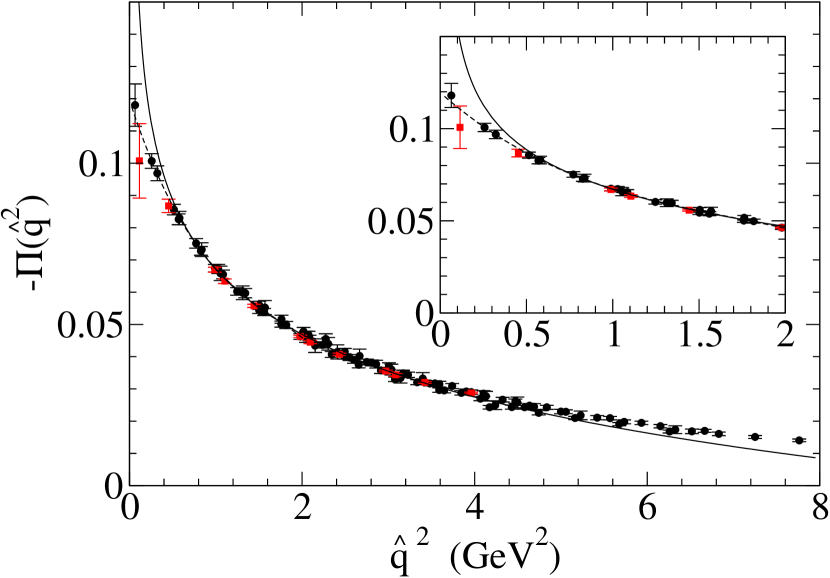
Shown in Figure 2 is the vacuum polarization for the large volume at GeV, the most physically interesting one since we are mainly interested in the small region. The agreement with perturbation theoryChetyrkin:1996cf is very good, even down to GeV2, until finally non-perturbative effects begin to be important. For very large values of lattice artifacts dominate, and the lattice and continuum results disagree. The perturbative result is evaluated in the scheme at GeV with a quark mass MeVDawson:2002nr and has been shifted by a constant333 The lattice and perturbative results are computed in different regularization schemes, and the logarithmic divergence has not been subtracted from the former. in Figure 2 for comparison. We also show the small volume results which indicate finite volume effects are negligible until GeV2. The results from the GeV lattice are quite similar, indicating that non-zero-lattice-spacing errors are small.
Since we are interested in the low region, to use Eq. 4, we fit the lattice data to a simple polynomial in , which allows for a smooth interpolation of the data. This amounts to a Taylor expansion about . Lorentz covariance (really, hyper-cubic symmetry) requires depend only on , and if the quark mass is non-zero, it must be regular as . A more sophisticated anastz is clearly desirable, especially one that includes finite volume effects. However, the construction of such an ansatz, for example in chiral perturbation theory, is outside the scope of this work. The value of between and the smallest value calculated on the lattice is extrapolated from the fit, so it is important to have values of that are close to zero. The smallest value in this study, which is on the large volume, is . Specifically, we use a four parameter fit function, where , and fit the data in the range GeV2. The fit is uncorrelated but performed under a jackknife procedure. The final results are insensitive to the number of parameters used and the fit range, so long as the chosen combination accurately reproduces the data. That is, the larger the range, the more parameters needed to accurately represent the low momentum region (see Figure 2).
The fit function is next plugged into Eq. 4 and integrated numerically, using MATHEMATICA, up to some cut, . The perturbative value of is then used in the integral from to , after it has been shifted by a constant to match onto the subtracted lattice result. The final result is quite insensitive to the value of the cut since in Eq. 4 is sharply peaked at zero, and with the statistical error on the present data such as it is, the perturbative contribution can be ignored entirely since it adds, depending on the cut, to . However, as the lattice results become more accurate, these contributions will have to be carefully included. To be specific, results are given for GeV2, though a much smaller value yields essentially the same answer.
Using the above procedure and including degenerate , , and quarks we find on the large volume (the error is statistical). This is roughly 2/3 of the value computed using the dispersive approachDavier:2002dy , and given the approximations in this first calculation: quenching, finite volume, and unphysically large quark masses, quite encouraging. We note with respect to the quenching systematic error, the above result is quite reasonable: 72% of the dispersive result comes directly from the resonanceDavier:2002dy , essentially all that is included in the quenched case. The result depends heavily on the low region, so the final statistical error is still rather large since only a small number of configurations were used (27) to compute averages over the gauge-field. The smaller volume result ( GeV, 138 configurations) is roughly , indicating large finite volume effects. The 1.96 GeV lattice, which corresponds to a somewhat larger volume, gives (18 configurations), in between the large and small 1.3 GeV lattices.
Since the hadronic loop is given by a sum over all possible values of the momentum of the quarks, one should worry that lattice artifacts due to finite may be noticable. Such effects were observed in domain wall fermion calculations of the chiral condensate and weak matrix elementsBlum:2000kn ; Blum:2001xb and are well understood. In the latter case, the physical matrix element was obtained by taking a slope with respect to quark mass which easily removed the lattice artifact. A similar mechanism is at work here. depends on through a constant, momentum independent shift which vanishes as , but the renormalized is independent of to a very high degree. This was checked by calculating with on the small volume, 1.3 GeV lattice. While the values of differ by roughly 30%, calculated with is in excellent agreement with the value. Being purely an issue of the physics near the ultraviolet cut-off where the heavy 5 fermions play a role (apart from the small additive quark mass, Blum:2000kn , which affects the low energy physics), this could have been anticipated from Figure 2. Since the agreement with perturbation theory is so good, visible effects would only show up as a constant.
We note that the vacuum polarization can also be fit to a form given by the operator product expansionGockeler:2000kj , though being a short distance expansion, it is valid for . In particular, in this (quenched) study we find no evidence for power corrections beyond the operator product expansion, which is in agreement with Gockeler:2000kj .
We are optimistic about the prospects for improving this calculation. Further quenched calculations on larger volumes will pin down finite volume effects, reduce the statistical error (there is room for significant improvement), and probe the chiral limit for the light quarks. The disconnected diagram that does not vanish in the non-degenerate case will also be computed. This should reduce the error on the quenched calculation below five percent. Recent simulations with dynamical domain wall fermionsIzubuchi:2002pt may be valuable in estimating the quenching error. Perhaps even more interesting in the near term, recent 2+1 flavor dynamical fermion calculations using improved Kogut-Susskind fermions444Private communication with Doug Toussaint of the MILC collaboration.Bernard:2002ep offer a promising avenue to address all the main systematic errors in this first calculation. The procedure set down here goes through in just the same way, but with dynamical gauge fields replacing the quenched ones. It is the generation of gauge fields with the dynamical fermion effects, especially for light quarks, that is so costly. Though we are still a ways from competing with the precision of the dispersive method, lattice calculations should eventually rival that precision. We have already mentioned that the lattice method avoids the problems of disentangling QED effects from the hadronic corrections, and isopin breaking can be handled simply by using different quark masses for the and quarks. In any case, a completely theoretical, first principles calculation, though challenging, is well worth the effort.
References
- (1) G. W. Bennett et al., Phys. Rev. Lett. 89, 101804 (2002).
- (2) M. Davier, S. Eidelman, A. Hocker, and Z. Zhang, Eur. Phys. J. C27, 497 (2003), eprint hep-ph/0208177.
- (3) K. Hagiwara, A. D. Martin, D. Nomura, and T. Teubner (2002), eprint hep-ph/0209187.
- (4) R. Z. Roskies, M. J. Levine, and E. Remiddi, Adv. Ser. Direct. High Energy Phys. 7, 162 (1990).
- (5) R. Barbieri, J. A. Mignaco, and E. Remiddi, Nuovo Cim. A11, 824 (1972).
- (6) M. E. Peskin and D. V. Schroeder , Reading, USA: Addison-Wesley (1995) 842 p.
- (7) T. Kinoshita, Adv. Ser. Direct. High Energy Phys. 7, 218 (1990).
- (8) D. B. Kaplan, Phys. Lett. B288, 342 (1992).
- (9) Y. Shamir, Nucl. Phys. B406, 90 (1993).
- (10) V. Furman and Y. Shamir, Nucl. Phys. B439, 54 (1995).
- (11) M. Gockeler et al., Nucl. Phys. Proc. Suppl. 94, 571 (2001), and references therein.
- (12) T. Takaishi, Phys. Rev. D54, 1050 (1996).
- (13) Y. Aoki et al. (2002), eprint hep-lat/0211023.
- (14) C. Dawson (RBC) (2002), eprint hep-lat/0210005.
- (15) K. G. Chetyrkin, J. H. Kuhn, and M. Steinhauser, Nucl. Phys. B482, 213 (1996).
- (16) T. Blum et al. (2000), eprint hep-lat/0007038.
- (17) T. Blum et al. (RBC) (2001), eprint hep-lat/0110075.
- (18) T. Izubuchi (RBC) (2002), eprint hep-lat/0210011.
- (19) C. Bernard et al. (MILC) (2002), eprint hep-lat/0209163.
Acknowledgments
I am grateful to W. Marciano for many useful discussions, and in particular for pointing out the work in Ref. Roskies:1990ki . I also thank M. Creutz, T. Izubuchi, and A. Soni for helpful discussions. I thank RIKEN, Brookhaven National Laboratory and the U.S. Department of Energy for providing the facilities essential for the completion of this work. All computations were carried out on the QCDSP supercomputers at the RIKEN BNL Research Center and Columbia University.