Spin on the lattice

Abstract

I review the current status of hadronic structure computations on the lattice. I describe the basic lattice techniques and difficulties and present some of the latest lattice results; in particular recent results of the RBC group using domain wall fermions are also discussed.

Understanding the basic properties of matter requires the understanding of the nucleon structure. Quantum Chromodynamics (QCD) is the theory describing strong interactions and hence is responsible for the properties of the nuclear matter. Although QCD has been around for more than twenty years, its non-perturbative nature is an obstacle to the direct connection of low energy physics to quarks and gluons, the fundamental degrees of freedom of the theory. Unlike QED, non-perturbative techniques had to be developed in order to understand the QCD predictions at low energies. The lattice formulation of QCD is both a non-perturbative way to define the theory and a very powerful tool in understanding its properties.

Deep inelastic scattering of leptons on nucleons has been an important tool in understanding the structure of hadrons. Over the last few decades experiments at SLAC, Fermilab, CERN, DESY, and more recently at RHIC and JLAB, have measured the quark and gluon light cone distribution functions of the nucleon. These experiments have substantially advanced our knowledge of the properties of hadrons. However, we would also like to study how this observed rich phenomenology arises form first principles, i.e. QCD. With todays advances in computer technology, algorithms, and recent developments in lattice regularization of fermions, lattice calculations can complement the experimental effort and promote our understanding of the non-perturbative nature of QCD.

0.1 The Lattice Formulation

The continuum Euclidean path integral can be defined using the lattice regulator Wilson (1974). In order to preserve gauge invariance the lattice gauge fields are link variables

$$U_{\mu}(x)=e^{i\int_{x}^{x+\hat{\mu}}d\tau A_{\mu}(\tau)},$$ (1)

where $A_{\mu}$ are the continuum gauge fields. The fermion fields live on the sites of the lattice. Naive discretization of the continuum fermionic action leads to the so-called fermion doubling problem. This problem can be avoided by either reinterpreting the additional light fermions as extra flavors (the Kogut-Susskind approach) or by introducing an irrelevant dimension 5 operator that breaks chiral symmetry on the lattice and gives mass proportional to the inverse lattice cutoff to the fermion doublers (the Wilson approach). Recently, new lattice fermionic actions that both preserve chiral symmetry on the lattice and do not suffer from the fermion doubling problem have been introduced. Such fermionic actions are the domain wall fermions Kaplan (1992, 1993); Shamir (1993); Furman and Shamir (1995), the overlap fermions Narayanan and Neuberger (1994), and the fixed point fermions DeGrand et al. (1995); Bietenholz and Wiese (1996); Hasenfratz et al. (2001). Having defined the lattice theory, correlation functions can be evaluated using Monte-Carlo integration in Euclidean space.

However, parton distribution functions are defined in the Minkowski space, and hence cannot be directly computed in lattice QCD. Using the operator product expansion we can relate moments of the structure functions to forward matrix elements of gauge invariant local operators (for a pedagogical review see Manohar (1992)). These matrix elements can then be computed using lattice QCD.

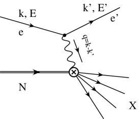
Figure 1: Deep inelastic scattering.

In a deep inelastic process (see Fig. 1) the cross section is given by

$$\frac{d^{2}\sigma}{d\Omega dE^{\prime}}=\frac{1}{2m_{N}}\frac{\alpha^{2}}{q^{4}}\frac{E^{\prime}}{E}l^{\mu\nu}W_{\mu\nu}$$ (2)

where $l^{\mu\nu}$ is the lepton tensor, $W_{\mu\nu}$ is the hadronic tensor, $q$ is the momentum transfer, $m_{N}$ is the nucleon mass. The initial and final energy and momentum of the lepton are ($E,k$) and ($E^{\prime},k^{\prime}$) respectively.

The hadronic tensor can be decomposed in the symmetric $W^{\{\mu\nu\}}$ and anti-symmetric $W^{[\mu\nu]}$ pieces:

$$W^{\mu\nu}=W^{[\mu\nu]}+W^{\{\mu\nu\}}$$ (3)

The symmetric piece defines the unpolarized structure functions $F_{1}$ and $F_{2}$ ($F_{3}$ also for neutrino scattering).

$$W^{\{\mu\nu\}}(x,Q^{2})=\left(-g^{\mu\nu}+\frac{q^{\mu}q^{\nu}}{q^{2}}\right)F_{1}(x,Q^{2})+\!\left(p^{\mu}-\frac{\nu}{q^{2}}q^{\mu}\right)\!\!\!\left(p^{\nu}-\frac{\nu}{q^{2}}q^{\nu}\right)\!\frac{F_{2}(x,Q^{2})}{\nu},$$

while the anti-symmetric defines the polarized structure functions $g_{1}$ and $g_{2}$

$$W^{[\mu\nu]}(x,Q^{2})=i\epsilon^{\mu\nu\rho\sigma}q_{\rho}\left(\frac{s_{\sigma}}{\nu}(g_{1}(x,Q^{2})+g_{2}(x,Q^{2}))-\frac{q\cdot sp_{\sigma}}{\nu^{2}}{g_{2}(x,Q^{2})}\right).$$ (4)

where $p_{\mu}$ and $s_{\mu}$ are the nucleon momentum and spin vectors, $\nu=q\cdot p$, $s^{2}=-m_{N}^{2}$, $x=Q^{2}/2\nu$ and $Q^{2}=-q^{2}$.

At the leading twist in the operator product expansion the moments of the structure functions can be factorized at a scale $\mu$ in hard perturbative contributions (the Wilson coefficients) and low energy matrix elements of local gauge invariant operators:

$$2\int_{0}^{1}dxx^{n-1}{F_{1}(x,Q^{2})} = \sum_{q=u,d}c^{(q)}_{1,n}(\mu^{2}/Q^{2},g(\mu))\>v_{n}^{(q)}(\mu),$$

$$\int_{0}^{1}dxx^{n-2}{F_{2}(x,Q^{2})} = \sum_{q=u,d}c^{(q)}_{2,n}(\mu^{2}/Q^{2},g(\mu))\>v_{n}^{(q)}(\mu),$$

$$2\int_{0}^{1}dxx^{n}{g_{1}(x,Q^{2})} = \frac{1}{2}\sum_{q=u,d}e^{(q)}_{1,n}(\mu^{2}/Q^{2},g(\mu))\>a_{n}^{(q)}(\mu),$$

$$2\int_{0}^{1}dxx^{n}{g_{2}(x,Q^{2})} = \frac{1}{2}\frac{n}{n+1}\sum_{q=u,d}[e^{(q)}_{2,n}(\mu^{2}/Q^{2},g(\mu))\>{d_{n}^{(q)}(\mu)}-$$ (5)

$$- e^{(q)}_{1,n}(\mu^{2}/Q^{2},g(\mu))\>a_{n}^{(q)}(\mu)]$$

where $c^{(q)}_{i,n},e^{(q)}_{i,n}$ are the Wilson coefficients and $v_{n}^{(q)}(\mu),a_{n}^{(q)},{d_{n}^{(q)}(\mu)}$ are the non-perturbative matrix elements. At the leading twist $v_{n}^{(q)}(\mu)$ and $a_{n}^{(q)}$ are related to the parton model distribution functions $\langle x^{n}\rangle_{q}$ and $\langle x^{n}\rangle_{\Delta q}$:

$$\langle x^{n-1}\rangle_{q}=v_{n}^{(q)}\;\;\;\;\;\;\;\;\;\;\;\;\;\;\;\langle x^{n}\rangle_{\Delta q}=\frac{1}{2}a_{n}^{(q)}$$ (6)

In order to extract $v_{n}^{(q)}(\mu),a_{n}^{(q)}$, and ${d_{n}^{(q)}(\mu)}$ we need to compute non-perturbatively the following matrix elements:

$$\frac{1}{2}\sum_{s}\langle p,s|{{\cal O}^{q}_{\{{\mu_{1}\mu_{2}\cdot\cdot\cdot\mu_{n}}\}}}|p,s\rangle = 2v_{n}^{(q)}(\mu)\times[p_{\mu_{1}}p_{\mu_{2}}\cdot\cdot\cdot p_{\mu_{n}}+\cdot\cdot\cdot-tr]$$

$$-\langle p,s|{{\cal O}^{5q}_{\{\sigma{\mu_{1}\mu_{2}\cdot\cdot\cdot\mu_{n}}\}}}|p,s\rangle = \frac{1}{n+1}a_{n}^{(q)}(\mu)\times[s_{\sigma}p_{\mu_{1}}p_{\mu_{2}}\cdot\cdot\cdot p_{\mu_{n}}+\cdot\cdot\cdot-tr]$$

$$\langle p,s|{\cal O}^{[5]q}_{[\sigma\{\mu_{1}]{\mu_{2}\cdot\cdot\cdot\mu_{n}}\}}|p,s\rangle = \frac{1}{n+1}{d_{n}^{q}}(\mu)\times[(s_{\sigma}p_{\mu_{1}}-s_{\mu_{1}}p_{\sigma})p_{\mu_{2}}\cdot\cdot\cdot p_{\mu_{n}}+\cdot\cdot\cdot-tr]$$

$\{\}$ implies symmetrization and $[]$ anti-symmetrization of indices. The nucleon states $|p,s\rangle$ are normalized so that $\langle p,s|p^{\prime},s^{\prime}\rangle=(2\pi)^{3}2E(p)\delta(p-p^{\prime})\delta_{s,s^{\prime}}$ and $s^{2}=-m^{2}_{N}$. The operators $\cal O$ are

$${\cal O}^{q}_{\mu_{1}\mu_{2}\cdot\cdot\cdot\mu_{n}} = \left(\frac{i}{2}\right)^{n-1}\bar{q}\gamma_{\mu_{1}}\stackrel{{\scriptstyle\,\leftrightarrow}}{{D}}_{\mu_{2}}\cdot\cdot\cdot\stackrel{{\scriptstyle\,\leftrightarrow}}{{D}}_{\mu_{n}}q-trace$$

$${\cal O}^{5q}_{\sigma{\mu_{1}\mu_{2}\cdot\cdot\cdot\mu_{n}}} = \left(\frac{i}{2}\right)^{n}\bar{q}\gamma_{\sigma}\gamma_{5}\stackrel{{\scriptstyle\,\leftrightarrow}}{{D}}_{\mu_{2}}\cdot\cdot\cdot\stackrel{{\scriptstyle\,\leftrightarrow}}{{D}}_{\mu_{n}}q-trace$$ (8)

where $\stackrel{{\scriptstyle\,\leftrightarrow}}{{D}}=\overrightarrow{D}-\overleftarrow{D}$ and $\overrightarrow{D}$, $\overleftarrow{D}$ are covariant derivatives acting on the right and the left respectively.

In Drell-Yan processes the transversity distribution $\langle x\rangle_{\delta q}$ can be measured (for details see Jaffe and Ji (1991, 1992); Barone et al. (2002)). The relevant matrix element is

$$\langle p,s|{{\cal O}^{\sigma q}_{\rho\nu\{{\mu_{1}\mu_{2}\cdot\cdot\cdot\mu_{n}}\}}}|p,s\rangle=\frac{2}{m_{N}}{\langle x^{n}\rangle_{\delta q}}(\mu)\times[(s_{\rho}p_{\nu}-s_{\nu}p_{\rho})p_{\mu_{1}}p_{\mu_{2}}\cdot\cdot\cdot p_{\mu_{n}}+\cdot\cdot\cdot-tr]$$

and the operators ${\cal O}^{\sigma q}$ are

$${{\cal O}^{\sigma q}_{\rho\nu{\mu_{1}\mu_{2}\cdot\cdot\cdot\mu_{n}}}}=\left(\frac{i}{2}\right)^{n}\bar{q}\gamma_{5}\sigma_{\rho\nu}\stackrel{{\scriptstyle\,\leftrightarrow}}{{D}}_{\mu_{1}}\cdot\cdot\cdot\stackrel{{\scriptstyle\,\leftrightarrow}}{{D}}_{\mu_{n}}q-trace.$$ (9)

0.2 Lattice matrix elements

In order to calculate on the lattice the needed matrix elements we have to compute nucleon three point functions

$$C^{\Gamma}_{3pt}(\vec{p},t,\tau)=\sum_{\alpha,\beta}\Gamma^{\alpha,\beta}\langle J_{\beta}(\vec{p},t){\cal O}(\tau)\bar{J}_{\alpha}(\vec{p},0)\rangle$$ (10)

and nucleon two point functions

$$C_{2pt}(\vec{p},t)=\sum_{\alpha,\beta}\left.\frac{1+\gamma_{4}}{2}\right|_{\alpha,\beta}\langle J_{\beta}(\vec{p},t)\bar{J}_{\alpha}(\vec{p},0)\rangle$$ (11)

where $\bar{J}(\vec{p},0)$ and $J(\vec{p},t)$ are creation and annihilation operators of states with the quantum numbers of the nucleon. For unpolarized matrix elements $\Gamma=\frac{1+\gamma_{4}}{2}$ while for the polarized $\Gamma=\frac{1+\gamma_{4}}{2}i\gamma_{5}\gamma_{k}$ ($k\neq 4$). The $\frac{1+\gamma_{4}}{2}$ factor is for projecting out the positive parity part of the baryon propagator i.e. the nucleon. For the proton a typical choice is

$$J_{\alpha}(\vec{p},t)=\sum_{\vec{x},a,b,c}e^{-i\vec{p}\cdot\vec{x}}\epsilon^{abc}\left[u^{a}(x,t)C\gamma_{5}d^{b}(x,t)\right]u^{c}_{\alpha}(x,t)$$ (12)

where $C=\gamma_{4}\gamma_{2}$ the charge conjugation matrix, $\alpha$ is a spinor index and $a,b,c$ are color indices. When $t\gg\tau\gg 0$

$$C_{2pt}(\vec{p},t) = Z_{N}\frac{E_{N}(\vec{p})+m_{N}}{E(\vec{p})}e^{-E_{N}(\vec{p})t}+\cdots$$

$$C^{\Gamma}_{3pt}(\vec{p},t,\tau) = Z_{N}\sum_{\alpha,\beta,s}\Gamma_{\alpha\beta}U^{\alpha}_{N}(p,s)\langle p,s|{\cal O}|p,s\rangle\bar{U}^{\beta}_{N}(p,s)e^{-E_{N}(\vec{p})t}+\cdots$$ (13)

where $U(p,s)$ is the nucleon spinor which satisfies the Dirac equation and $\langle 0|J_{\alpha}(\vec{p},t)|p,s\rangle=\sqrt{Z_{N}}U^{\alpha}(p,s)$. From Eq. 13 and Eq. LABEL:eq:matel (or Eq. 0.1) the required matrix elements can be extracted from the ratio of three point functions over two point functions. In practice we would like to achieve the asymptotic behavior of Eq. 13 with as small as possible $t$ and $\tau$. For that reason the interpolating operator $J$ is tuned so that the overlap with the exited nucleon states would be as small as possible. For more details on the technical aspects of the lattice calculation the reader may refer to Martinelli and Sachrajda (1989); Gockeler et al. (1996a, 2001); Dolgov et al. (2002).

In order to reduce the computational cost of calculating the above correlation functions some times the so-called quenched approximation is used. In this approximation the quark loop contributions to the path integral are ignored. Quenching reduces the computational cost by several orders of magnitude, while for certain quantities it introduces a systematic error $\sim 10\%$. In addition, lattice computations are typically performed with heavier quark masses than the physical up and down quarks. Hence we have to perform extrapolations to the chiral limit. If the quark masses are light enough, chiral perturbation theory Arndt and Savage (2002); Chen and Ji (2001); Chen and Savage (2002) can be used to calculate the dependence of the matrix elements on the quark mass. Finally the lattice matrix elements have to be renormalized, typically to $\overline{\rm MS}$, and extrapolated to the continuum limit.

0.3 Renormalization

The renormalized operators at scale $\mu$ are obtained from the lattice operators calculated at lattice spacing $a$ from

$${\cal O}^{ren}(\mu)=Z(\mu;a){\cal O}^{lat}(a)$$ (14)

in the case of multiplicatively renormalized operators. In general, there is operator mixing and as a result the above relation becomes

$${\cal O}_{i}^{ren}(\mu)=Z(\mu;a)\left[{\cal O}^{lat}_{i}(a)+\sum_{j\neq i}a^{d_{j}-d_{i}}Z_{ij}(\mu;a){\cal O}^{lat}_{j}(a)\right],$$ (15)

where ${\cal O}_{j}$ are a set of operators allowed by symmetries to mix, and $d_{j}$ is the dimension of each operator. It is evident that if mixing with lower dimensional operators occur, the mixing coefficients are power divergent as we approach the continuum limit. Hence we have to compute these terms non-perturbatively in order to accurately renormalize the operators. Higher dimensional operators are typically ignored since their effects vanish in the continuum limit. In certain cases we may want to compute these coefficients in order to remove part of the systematic error introduced by the finite cutoff.

The mixing of lattice operators is more complicated than that of the continuum operators, since on the lattice we do not have all the continuum symmetries. In particular, $O(4)$ rotational symmetry in Euclidean space is broken down to the hypercubic group $H(4)$. As a result, an irreducible representation of $O(4)$ is reducible under $H(4)$ and hence mixing of operators that would not occur in the continuum can occur on the lattice. For a detailed analysis of the $H(4)$ group representations see Mandula et al. (1983); Gockeler et al. (1996b) and references therein. In lattice calculations we have to select carefully the lattice operators so that mixing with lower dimensional operators does not occur and hence no power divergent coefficients in Eq. 15 are encountered. This turns out to be a significant constraint on how many moments can be practically computed on the lattice.

Another symmetry that is broken on the lattice for Wilson fermions is chiral symmetry. This results in mixings with lower dimensional operators for the $d_{n}$ matrix elements. Fortunately, in this case we can use lattice fermions, such as domain wall or overlap and fixed point fermions, that respect chiral symmetry on the lattice. For Wilson fermions, the renormalization of $d_{2}$ has been done non-perturbatively as described in Gockeler et al. (2001).

The renormalization constants for all the operators relevant to structure function calculations have been computed perturbatively for Wilson fermions, improved and unimproved Capitani and Rossi (1995); Beccarini et al. (1995); Capitani et al. (2001). Moreover, the RI-MOM scheme has been used to renormalize non-perturbatively both local Martinelli et al. (1995) and derivative operators Gockeler et al. (1999); Capitani et al. (2002). In the Schroedinger functional scheme (developed by the ALPHA collaboration), all local operator renormalizations and the renormalization of $v_{2}$ have been computed Guagnelli et al. (1999, 2000). In addition, work is underway for computing the constants for flavor singlet operators Palombi et al. (2002). For domain wall fermions, all local operators have been renormalized non-perturbatively Blum et al. (2002) using the RI-MOM scheme, and also perturbatively Aoki et al. (1999).

1 Lattice results

In the last several years, the lattice community (QCDSF/UKQCD and LHP/SESAM collaborations) has made a substantial effort to compute the first few moments of the nucleon structure functions. Apart from the constraints imposed by the renormalization of the operators mentioned above, the requirement of having nucleon states with non-zero momentum limits the number of moments we can compute. These are the first three moments of the unpolarized structure functions, the first two moments of the polarized structure functions, and the first two moments of the transversity. These computations have been performed both in quenched and in full QCD with improved and unimproved Wilson fermions Gockeler et al. (1996a, 1997, 2001); Dolgov et al. (2002).

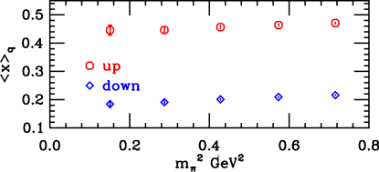
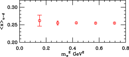
Figure 2: Quark density $\langle x\rangle_{q}$ vs. the pion mass squared. [left] The connected up (octagons) and down (diamonds) quark contributions. [right] The flavor non-singlet $\langle x\rangle_{u-d}$.

The RBC group has recently begun quenched computations with domain wall fermions Orginos (2002a). Our current results are restricted only to those matrix elements that can be computed with zero momentum nucleon states. We use the DBW2 gauge action which is known to improve the domain wall fermion chiral properties Orginos (2002b); Aoki (2002). We have 416 lattices of size $16^{3}\times 32$ at $\beta=0.870$ with lattice spacing $a^{-1}=1.3\rm GeV$, providing us with a physical volume ($\sim(2.4fm)^{3}$) large enough to reduce finite size effects known to affect some nucleon matrix elements, such as $g_{A}$ Sasaki et al. (2002); Ohta (2002). Using fifth dimension length $L_{s}=16$ we achieve a residual mass $m_{\rm res}\sim 0.8\rm MeV$ Orginos (2002b); Aoki (2002). The input quark masses ranged from $0.02$ to $0.10$, providing pion masses ranging from $390\rm MeV$ to $850\rm MeV$. Further technical details of our calculation can be found in Orginos (2002a).

1.1 Unpolarized Structure Functions

The first three moments of the unpolarized structure functions have been computed by QCDSF in the quenched approximation. The needed chiral and continuum extrapolations have also been performed. A summary of recent results can be found in Gockeler et al. (2002a). In comparison with MRS phenomenological results, the lattice results are typically higher. Also, $v_{3}$ is smaller than $v_{4}$, while $v_{3}>v_{4}$ is phenomenologically expected. The same computations have been performed by LHP/SESAM in full QCD Dolgov et al. (2002). Their results indicate that dynamical fermions have only a small effect on the matrix elements they studied.

It has been argued that the main reason for such discrepancies is the fact that lattice computations are performed at rather heavy quark masses and then extrapolated linearly to the chiral limit Detmold et al. (2001, 2002); Thomas (2002). For that reason, we need computations at much lighter quark masses in order to see whether there is a disagreement with phenomenological expectations. In quenched QCD, a study with very light quark masses has been done Gockeler et al. (2002b) indicating that the linear behavior persists down to 300MeV pion masses.

In Fig. 2 we present our results for the quark density distribution $\langle x\rangle_{q}$ ($v_{2}$). We plot the unrenormalized result for $\langle x\rangle_{u}$, $\langle x\rangle_{d}$ and the flavor non-singlet $\langle x\rangle_{u-d}$. Down to 380MeV pion mass no significant curvature within our statistical errors can be seen. The ratio ${\langle x\rangle_{u}}/{\langle x\rangle_{d}}$ is $2.41(4)$, linearly extrapolated to the chiral limit, is in agreement with the quenched Wilson fermion results Gockeler et al. (1996a); Dolgov et al. (2002).

1.2 Polarized Structure Functions

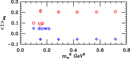
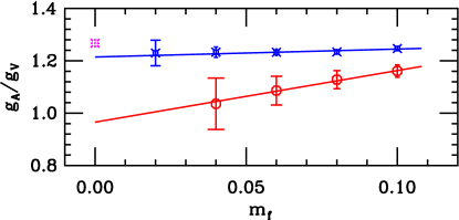
Figure 3: Helicity $\langle 1\rangle_{\Delta q}$ vs. the pion mass squared. [left] The connected up (octagons) and down (diamonds) quark contributions. [right] The nucleon axial charge $g_{A}$ i.e. flavor non-singlet $\langle 1\rangle_{\Delta u-\Delta d}$.

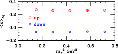
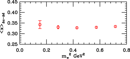
Figure 4: Helicity $\langle x\rangle_{\Delta q}$ vs. the pion mass squared. [left] The connected up (octagons) and down (diamonds) quark contributions. [right] The flavor non-singlet $\langle x\rangle_{\Delta u-\Delta d}$.

The nucleon axial charge $g_{A}$ is related to the first moment of the polarized structure function $g_{1}$. The current experimental value for $g_{A}/g_{V}$ measured from neutron beta decays is 1.2670(30) Hagiwara et al. (2002). Lattice calculations, quenched and dynamical, have been underestimating this quantity typically by 10% to 20% Fukugita et al. (1995); Gockeler et al. (1996a); Gusken et al. (1999); Gockeler et al. (2001); Dolgov et al. (2002); Gockeler et al. (2002a). For earlier calculations see also Liu et al. (1994); Dong et al. (1995).

One of the systematic errors believed to affect these calculations is the finite volume. In order to study this effect we performed two calculations. One with spatial volume $2.4^{3}fm^{3}$ and another with spatial volume $1.2^{3}fm^{3}$. Our results are shown in Fig. 3[right]. Between these two volumes it is clear that there is a finite volume effect of about 20% at the chiral limit. In addition, the linearly extrapolated to the chiral limit value for $g_{A}/g_{V}$ is 1.21(2). For a detailed analysis of this computation see Ohta (2002). Note that for domain wall fermions $g_{A}/g_{V}$ does not require renormalization, since the finite renormalization constants of the axial and the vector currents $Z_{A}$, $Z_{V}$ are equal Blum et al. (2002); Dawson (2002). In Fig. 3[left] we present the up and down quark contributions of $\langle 1\rangle_{\Delta q}$ for the proton renormalized using $Z_{A}=.77759(45)$ Aoki (2002). In Fig. 4 we present our unrenormalized data for $\langle x\rangle_{\Delta q}$. The ratio ${\langle x\rangle_{\Delta u}}/{\langle x\rangle_{\Delta d}}$ linearly extrapolated to the chiral limit is roughly $-4$, consistent with other lattice results Gockeler et al. (2001); Dolgov et al. (2002).

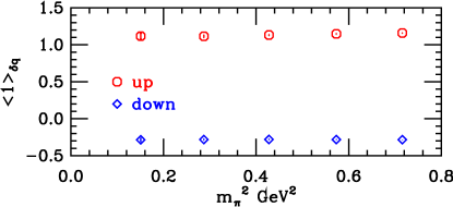
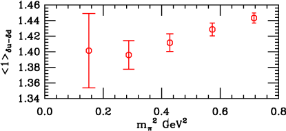
Figure 5: Transversity $\langle 1\rangle_{\delta q}$ vs. the pion mass squared. [left] The connected up (octagons) and down (diamonds) quark contributions. [right] The flavor non-singlet $\langle 1\rangle_{\delta u-\delta d}$.

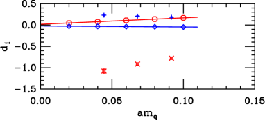
Figure 6: The connected $d_{1}$ matrix element vs. quark mass for the up (octagons) and down (diamonds) quarks. The up (fancy squares) and down (fancy diamonds) quark for Wilson fermions Dolgov et al. (2002).

The lowest moment of the transversity $\langle 1\rangle_{\delta q}$ is also measured. In Fig. 5 we plot the unrenormalized contributions for both the up and down quark, and the flavor non-singlet combination $\langle 1\rangle_{\delta u-\delta d}$. Again the quark mass dependence is very mild and there is no sign of a chiral log behavior. The ratio ${\langle 1\rangle_{\delta u}}/{\langle 1\rangle_{\delta d}}$ linearly extrapolated to the chiral limit is also roughly $-4$.

For computing moments of $g_{2}$ we need to calculate the twist 3 matrix elements $d_{n}$. We computed the $d_{1}$ matrix element which contributes to the first moment of $g_{2}$. If chiral symmetry is broken the operator ${\cal O}^{[5]q}_{34}=\frac{1}{4}\bar{q}\gamma_{5}\left[\gamma_{3}\stackrel{{\scriptstyle\,\leftrightarrow}}{{D}}_{4}-\gamma_{4}\stackrel{{\scriptstyle\,\leftrightarrow}}{{D}}_{3}\right]q$ which is used to compute $d_{1}$ mixes with the lower dimensional operator ${\cal O}^{\sigma q}_{34}=\bar{q}\gamma_{5}\sigma_{34}q.$ Hence in Wilson fermion calculations a non perturbative subtraction has to be performed. This has been done for $d_{2}$ by QCDSF Gockeler et al. (2001, 2002a). With domain wall fermions this kind of mixing is proportional to the residual mass ($\sim m_{\rm res}/a$), which in our case is negligible. Thus we expect that a straightforward computation of $d_{1}$ with domain wall fermions provides directly the physically interesting result. In Fig. 6 we present our unrenormalized results for $d_{1}$ as a function of the quark mass. For comparison we also plot the unsubtracted quenched Wilson results for $\beta=6.0$ from Dolgov et al. (2002). The fact that our result almost vanishes at the chiral limit is an indication that the power divergent mixing is absent for domain wall fermions. The behavior we find for the $d_{1}$ matrix element is consistent with that of the subtracted $d_{2}$ computed by QCDSF Gockeler et al. (2001, 2002a) with Wilson fermions.

2 Conclusions

In conclusion, lattice computations can play an important role in understanding the hadronic structure and the fundamental properties of QCD. Although some difficulties still exist, several significant steps have been made. Advances in computer technology are expected to play a significant role in pushing these computations closer to the chiral limit and in including dynamical fermions. RBC has already begun preliminary dynamical domain wall fermion computations Izubuchi (2002) which we expect to be pushed forward with the arrival of QCDOC Boyle et al. (2002). In the near future, we also expect to complete the non-perturbative renormalization of the relevant derivative operators in quenched QCD.

References

- Wilson (1974) Wilson, K. G., Phys. Rev., D10, 2445–2459 (1974).
- Kaplan (1992) Kaplan, D. B., Phys. Lett., B288, 342–347 (1992).
- Kaplan (1993) Kaplan, D. B., Nucl. Phys. Proc. Suppl., 30, 597–600 (1993).
- Shamir (1993) Shamir, Y., Nucl. Phys., B406, 90–106 (1993).
- Furman and Shamir (1995) Furman, V., and Shamir, Y., Nucl. Phys., B439, 54–78 (1995).
- Narayanan and Neuberger (1994) Narayanan, R., and Neuberger, H., Nucl. Phys., B412, 574–606 (1994).
- DeGrand et al. (1995) DeGrand, T., Hasenfratz, A., Hasenfratz, P., and Niedermayer, F., Nucl. Phys., B454 (1995).
- Bietenholz and Wiese (1996) Bietenholz, W., and Wiese, U. J., Nucl. Phys., B464, 319–352 (1996).
- Hasenfratz et al. (2001) Hasenfratz, P., et al., Int. J. Mod. Phys., C12, 691–708 (2001).
- Manohar (1992) Manohar, A. V., Proceedings of the Seventh Lake Louis Winter Institute (World Scientific) (1992).
- Jaffe and Ji (1991) Jaffe, R. L., and Ji, X.-D., Phys. Rev. Lett., 67, 552–555 (1991).
- Jaffe and Ji (1992) Jaffe, R. L., and Ji, X.-D., Nucl. Phys., B375, 527–560 (1992).
- Barone et al. (2002) Barone, V., Drago, A., and Ratcliffe, P. G., Phys. Rept., 359, 1–168 (2002).
- Martinelli and Sachrajda (1989) Martinelli, G., and Sachrajda, C. T., Nucl. Phys., B316, 355 (1989).
- Gockeler et al. (1996a) Gockeler, M., et al., Phys. Rev., D53, 2317–2325 (1996a).
- Gockeler et al. (2001) Gockeler, M., et al., Phys. Rev., D63, 074506 (2001).
- Dolgov et al. (2002) Dolgov, D., et al., Phys. Rev., D66, 034506 (2002).
- Arndt and Savage (2002) Arndt, D., and Savage, M. J., Nucl. Phys., A697, 429–439 (2002).
- Chen and Ji (2001) Chen, J.-W., and Ji, X.-d., Phys. Lett., B523, 107–110 (2001).
- Chen and Savage (2002) Chen, J.-W., and Savage, M. J., Nucl. Phys., A707, 452–468 (2002).
- Mandula et al. (1983) Mandula, J. E., Zweig, G., and Govaerts, J., Nucl. Phys., B228, 109 (1983).
- Gockeler et al. (1996b) Gockeler, M., et al., Phys. Rev., D54, 5705–5714 (1996b).
- Capitani and Rossi (1995) Capitani, S., and Rossi, G., Nucl. Phys., B433, 351–389 (1995).
- Beccarini et al. (1995) Beccarini, G., Bianchi, M., Capitani, S., and Rossi, G., Nucl. Phys., B456, 271–295 (1995).
- Capitani et al. (2001) Capitani, S., et al., Nucl. Phys., B593, 183–228 (2001).
- Martinelli et al. (1995) Martinelli, G., Pittori, C., Sachrajda, C. T., Testa, M., and Vladikas, A., Nucl. Phys., B445 (1995).
- Gockeler et al. (1999) Gockeler, M., et al., Nucl. Phys., B544, 699–733 (1999).
- Capitani et al. (2002) Capitani, S., et al., Nucl. Phys. Proc. Suppl., 106, 299–301 (2002).
- Guagnelli et al. (1999) Guagnelli, M., Jansen, K., and Petronzio, R., Phys. Lett., B459, 594–598 (1999).
- Guagnelli et al. (2000) Guagnelli, M., Jansen, K., and Petronzio, R., Phys. Lett., B493, 77–81 (2000).
- Palombi et al. (2002) Palombi, F., Petronzio, R., and Shindler, A., Nucl. Phys., B637, 243–271 (2002).
- Blum et al. (2002) Blum, T., et al., Phys. Rev., D66, 014504 (2002).
- Aoki et al. (1999) Aoki, S., Izubuchi, T., Kuramashi, Y., and Taniguchi, Y., Phys. Rev., D60, 114504 (1999).
- Gockeler et al. (1997) Gockeler, M., et al., Phys. Lett., B414, 340–346 (1997).
- Orginos (2002a) Orginos, K., Nucl. Phys. Proc. Suppl. (Lattice 2002) (2002a).
- Orginos (2002b) Orginos, K., Nucl. Phys. Proc. Suppl., 106, 721–723 (2002b).
- Aoki (2002) Aoki, Y., Nucl. Phys. Proc. Suppl., 106, 245–247 (2002).
- Sasaki et al. (2002) Sasaki, S., Blum, T., Ohta, S., and Orginos, K., Nucl. Phys. Proc. Suppl., 106, 302–304 (2002).
- Ohta (2002) Ohta, S., Nucl. Phys. Proc. Suppl. (Lattice 2002) (2002).
- Gockeler et al. (2002a) Gockeler, M., et al., Nucl. Phys. Proc. Suppl. (Lattice 2002) (2002a).
- Detmold et al. (2001) Detmold, W., Melnitchouk, W., Negele, J. W., Renner, D. B., and Thomas, A. W., Phys. Rev. Lett., 87, 172001 (2001).
- Detmold et al. (2002) Detmold, W., Melnitchouk, W., and Thomas, A. W., Phys. Rev., D66, 054501 (2002).
- Thomas (2002) Thomas, A. W., Nucl. Phys. Proc. Suppl. (Lattice 2002) (2002).
- Gockeler et al. (2002b) Gockeler, M., Horsley, R., Pleiter, D., Rakow, P. E. L., and Schierholz, G., Nucl. Phys. Proc. Suppl. (Lattice 2002) (2002b).
- Hagiwara et al. (2002) Hagiwara, K., et al., Phys. Rev., D66, 010001 (2002).
- Fukugita et al. (1995) Fukugita, M., Kuramashi, Y., Okawa, M., and Ukawa, A., Phys. Rev. Lett., 75, 2092–2095 (1995).
- Gusken et al. (1999) Gusken, S., et al., Phys. Rev., D59, 114502 (1999).
- Liu et al. (1994) Liu, K. F., Dong, S. J., Draper, T., Wu, J. M., and Wilcox, W., Phys. Rev., D49, 4755–4761 (1994).
- Dong et al. (1995) Dong, S. J., Lagae, J. F., and Liu, K. F., Phys. Rev. Lett., 75, 2096–2099 (1995).
- Dawson (2002) Dawson, C., Nucl. Phys. Proc. Suppl. (Lattice 2002) (2002).
- Izubuchi (2002) Izubuchi, T., Nucl. Phys. Proc. Suppl. (Lattice 2002) (2002).
- Boyle et al. (2002) Boyle, P. A., et al., Nucl. Phys. Proc. Suppl. (Lattice 2002) (2002).