Domain wall fermions with improved gauge actions

Abstract

We study the chiral properties of quenched domain wall fermions with several gauge actions. We demonstrate that the residual chiral symmetry breaking, which is present for a finite number of lattice sites in the fifth dimension ($L_{s}$), can be substantially suppressed using improved gauge actions. In particular the Symanzik action, the Iwasaki action, and a renormalization group improved gauge action, called doubly blocked Wilson (DBW2), are studied and compared to the Wilson action. All improved gauge actions studied show a reduction in the additive residual quark mass, $m_{\rm res}$. Remarkably, in the DBW2 case $m_{\rm res}$ is roughly two orders of magnitude smaller than the Wilson gauge action at $a^{-1}=2$ GeV and $L_{s}=16$. Significant reduction in $m_{\rm res}$ is also realized at stronger gauge coupling corresponding to $a^{-1}=1.3$ GeV. As our numerical investigation indicates, this reduction is achieved by reducing the number of topological lattice dislocations present in the gauge field configurations. We also present detailed results for the quenched light hadron spectrum and the pion decay constant using the DBW2 gauge action.

I Introduction

Domain wall fermions Kaplan (1992, 1993); Shamir (1993); Furman and Shamir (1995) are expected to provide an implementation of lattice fermions with exact chiral symmetry, even at a finite lattice spacing. To achieve this exact symmetry, an infinite fifth dimension must be introduced and simulations have been done to explore the limit of large fifth dimension for both full and quenched QCD Blum et al. (2000); Ali Khan et al. (2001); Aoki and Taniguchi (2002); Chen et al. (2001); Izubuchi and Dawson (2002); Izubuchi (2002). The finite size of the fifth dimension, $L_{s}$, used in numerical simulations, produces a small amount of chiral symmetry breaking, which should go to zero in the limit $L_{s}\to\infty$. In practical implementations the aim is to achieve the smallest chiral symmetry breaking possible at a given $L_{s}$, thus minimizing the cost of the simulation. Further information about domain wall fermions and their applications is given in the recent reviews Vranas (2001); Hernandez (2002).

There have now been several suggestions on how to minimize the computational cost of domain wall fermions. An obvious way to achieve this is to make the five-dimensional eigenvectors of the domain wall fermion operator, which for small eigenvalues should be localized on the four-dimensional boundaries of the fifth dimension, decay faster in the fifth dimension. This reduces the mixing between the opposite chirality modes, which are bound to opposite ends of the fifth dimension. Shamir Shamir (2000) has calculated the fifth-dimensional decay of the eigenfunctions with zero eigenvalues using perturbation theory, suggesting a modification of the four-dimensional component of the domain wall fermion operator to increase the decay. This interesting perturbative result may explain some of the features seen in non-perturbative simulations. (Of course, modifications to the domain wall fermion operator may increase the computational cost by more than the reduction in $L_{s}$ reduces it.) Another method of improving domain wall fermions is proposed in Edwards and Heller (2001); Hernandez et al. (2000). The basic idea behind these proposals is to project out the zero modes of the four-dimensional Hamiltonian describing the propagation in the fifth dimension. As a result, the localization on the boundaries of the fermionic light modes is enhanced.

In this paper we systematically examine a different option: the modification of the gauge action to suppress the finite $L_{s}$ explicit chiral symmetry breaking Orginos (2002). Note that in principle this is a different criteria from improving the gauge action to achieve better scaling, in lattice spacing, of physical observables. We will investigate the scaling of observables as well, to check that while reducing the explicit chiral symmetry breaking, we do not distort the approach to the continuum limit. It is worth noting that methods which improve the domain wall fermion operator, like those suggested by Shamir, and the one investigated here are likely independent of each other, so a combination of both techniques may lead to even greater efficiency in domain wall fermion simulations. However, as we will see, our approach obviates the need of separately treating the near unit eigenvectors of the transfer matrix, as gauge configurations for which these occur are suppressed. This has also been studied in Hernandez et al. (2002).

The observation that the gauge action can affect significantly the chiral symmetry of domain wall fermions is not new. Both the RBC Wu (2000) and CP-PACS Ali Khan et al. (2000, 2001) collaborations have observed that the use of the Iwasaki action Iwasaki (1983) substantially improves chiral symmetry in quenched simulations. Also in Jung et al. (2001) it was observed that the 1-loop Symanzik Alford et al. (1995) improved gauge action improves chiral symmetry to a lesser degree. Here we extend these results and explore the reason behind the observed improvement.

This paper is organized as follows. In section II we give a brief description of the gauge actions under study. In section III we introduce the observables used for studying chiral symmetry breaking and also present the standard Wilson action results to provide a reference point. Section IV contains results for the different actions we studied. We find that the doubly blocked Wilson (DBW2) action Takaishi (1996); de Forcrand et al. (2000) gives residual chiral symmetry breaking two orders of magnitude smaller than the Wilson gauge action at comparable lattice spacings and values of $L_{s}$. In section V we discuss the dominant mechanism of explicit chiral symmetry breaking in domain wall fermions, which we find is driven by lattice artifacts, or dislocations, at the lattice spacings considered. These dislocations occur as the topological charge of the gauge field configuration changes during Monte Carlo evolution. Given this large improvement in residual chiral symmetry breaking and the fact that the DBW2 action has not been used before with domain wall fermions, in Section VI we present results for some hadronic observables in order to confirm consistency with quenched simulations using other gauge actions, to check scaling with lattice spacing and to lay a foundation for future work Aoki (2002).

II Pure Gauge Lattice Actions

As mentioned, we study the chiral properties of quenched domain wall fermions with Symanzik, Iwasaki, and DBW2 gauge actions. These actions are built from closed loops of up to six links and provide a sample of typical lattice actions used to improve scaling of observables. As a baseline for comparisons we start with the Wilson action Wilson (1974) which is defined by

$$S_{G}[U]=-\frac{\beta}{3}\sum_{x;\mu<\nu}P[U]_{x,\mu\nu}$$ (1)

where $P[U]_{x,\mu\nu}$ is the real part of the trace of the path ordered product of links around the $1\times 1$ plaquette in the $\mu,\nu$ plane at point $x$ and $\beta\sim 1/g^{2}_{0}$ with $g_{0}$ the bare gauge coupling. This is the original non-abelian gauge action introduced by Wilson, which has ${\cal O}(a^{2})$ errors ($a$ is the lattice spacing).

To begin, we study the Symanzik one loop improved action Alford et al. (1995) where both ${\cal O}(a^{2})$ and ${\cal O}(g^{2}a^{2})$ errors are removed. This action is defined as

$$S_{G}[U]=-\frac{\beta}{3}\left(c_{0}\sum_{x;\mu<\nu}P[U]_{x,\mu\nu}+c_{1}\sum_{x;\mu\neq\nu}R[U]_{x,\mu\nu}+c_{2}\sum_{x;\mu<\nu<\sigma}C[U]_{x,\mu\nu\sigma}\right)$$ (2)

where $R[U]_{x,\mu\nu}$ and $C[U]_{x,\mu\nu\sigma}$ denote the real part of the trace of the ordered product of SU(3) link matrices along $1\times 2$ rectangles in the $\mu,\nu$ plane and the $\mu,\nu,\sigma,-\mu,-\nu,-\sigma$ paths, respectively. The coefficients $c_{0}$, $c_{1}$, and $c_{2}$ are computed in tadpole improved one loop perturbation theory Alford et al. (1995). For this action and the remaining ones, $\beta\sim 1/g^{2}_{0}$ as for the Wilson action, but the precise numerical factors differ.

In addition to the above actions we also studied the Iwasaki Iwasaki (1983) action and the DBW2 action Takaishi (1996); de Forcrand et al. (2000). These actions are both renormalization group (RG) improved actions in a truncated, two-parameter space. They can be written down as

$$S_{G}[U]=-\frac{\beta}{3}\left((1-8\,c_{1})\sum_{x;\mu<\nu}P[U]_{x,\mu\nu}+c_{1}\sum_{x;\mu\neq\nu}R[U]_{x,\mu\nu}\right)$$ (3)

with $c_{1}=-0.331$ for the Iwasaki action and $c_{1}=-1.4069$ for the DBW2 action. In the case of the Iwasaki action the coefficient $c_{1}$ is computed in weak coupling perturbation theory. For the DBW2 action $c_{1}$ is computed Takaishi (1996) non-perturbatively using Swendsen’s blocking and the Schwinger-Dyson method. QCD-TARO has studied de Forcrand et al. (2000) the RG flow in the two parameter space of the plaquette and the rectangle couplings and concluded that DBW2 is a good approximation to the RG flow in this plane at least for a range of coarse lattice spacings.

Although the Iwasaki and DBW2 actions are motivated by the desire to remain on the RG trajectory for quenched QCD, the truncation to the explicit form used is an approximation. The accuracy with which these truncated actions preserve the RG trajectory must be investigated numerically. Simulations with the Iwasaki action Iwasaki et al. (1997) and the DBW2 action de Forcrand et al. (2000) show improved scaling of the heavy quark potential and the critical temperature for the finite temperature phase transition, compared to the Wilson gauge action. These actions serve as useful starting points for studying the effects of the gauge action on residual chiral symmetry breaking in domain wall fermions.

III Explicit Chiral Symmetry Breaking with Domain Wall Fermions

The central idea behind domain wall fermions is that four-dimensional fermionic states of opposite chirality are localized dynamically on opposite boundaries of an extra fifth dimension. The domain wall fermions are coupled to four-dimensional gauge fields replicated in the fifth direction, so the light states can be used to simulate a vector gauge theory like QCD. The five-dimensional fermion action is a generalization of the Wilson fermion action Wilson (1974) with open boundary conditions in the fifth dimension Shamir (1993). In the free field limit, localization of a single fermionic flavor on the four-dimensional boundaries occurs if the five-dimensional fermion mass $M_{5}$ is in the interval (0,2). This interval is shifted when interactions are switched on. For an infinite fifth dimension ($L_{s}\rightarrow\infty$), chiral symmetry of the light states is manifest since they have no overlap. Four-dimensional light quark $q,\overline{q}$ fields are constructed from the five-dimensional fermions $\Psi,\overline{\Psi}$ by

$$q(x) = P_{L}\Psi(x,0)+P_{R}\Psi(x,L_{s}-1)$$ (4)

$$\overline{q}(x) = \overline{\Psi}(x,L_{s}-1)P_{L}+\overline{\Psi}(x,0)P_{R},$$ (5)

where $P_{R/L}=\frac{1}{2}(1\pm\gamma_{5})$ are the right-handed and left-handed projection operators. Hence a four-dimensional mass term $m_{f}\overline{q}q$ can be introduced if the fifth dimension boundaries are coupled directly with a parameter $m_{f}$Shamir (1993). For finite $L_{s}$ explicit chiral symmetry breaking is induced by the mixing of the light states which now extend across the fifth dimension. Our conventions throughout this paper are the same as those in Blum et al. (2000).

In order to quantify the explicit chiral symmetry breaking induced at finite $L_{s}$, we define the residual mass ($m_{res}$) through the Ward-Takahashi identity Furman and Shamir (1995):

$$\Delta_{\mu}\langle{\cal A}^{a}_{\mu}(x)O(y)\rangle=2m_{f}\langle J^{a}_{5}(x)O(y)\rangle+2\langle J^{a}_{5q}(x)O(y)\rangle+i\langle\delta^{a}O(y)\rangle,$$ (6)

where

$${\cal A}^{a}_{\mu}(x)=\sum_{s=0}^{L_{s}-1}{\rm sign}\left(s-\frac{L_{s}-1}{2}\right)j^{a}_{\mu}(x,s)$$ (7)

is a four-dimensional partially-conserved axial current which is constructed from the five-dimensional conserved vector current,

$$j^{a}_{\mu}(x,s)=\frac{1}{2}\left[\overline{\Psi}(x+\hat{\mu},s)(1+\gamma_{\mu})U^{\dagger}_{x+\hat{\mu},\mu}t^{a}\Psi(x,s)-\overline{\Psi}(x,s)(1-\gamma_{\mu})U_{x,\mu}t^{a}\Psi(x+\hat{\mu},s)\right].$$ (8)

The flavor matrices are normalized to obey ${\rm Tr}\,(t^{a}t^{b})=\delta^{ab}$, $\Delta_{\mu}f(x)=f(x)-f(x-\hat{\mu})$ is a simple finite difference operator, and the pseudoscalar density $J^{a}_{5}(x)$ is

$$J^{a}_{5}(x) = -\overline{\Psi}(x,L_{s}-1)P_{\rm L}t^{a}\Psi(x,0)+\overline{\Psi}(x,0)P_{\rm R}t^{a}\Psi(x,L_{s}-1).$$ (9)

Note that $J^{a}_{5}(x)$ is a four-dimensional pseudoscalar density constructed from fields on the boundaries of the fifth dimension. The identity (6) differs from the continuum expression by the presence of the $J^{a}_{5q}(x)$ term. $J^{a}_{5q}(x)$ is analogous to $J^{a}_{5}(x)$, but is built from fields in the bulk at $L_{s}/2$ and $L_{s}/2-1$.

$$J^{a}_{5q}(x)=-\overline{\Psi}(x,L_{s}/2-1)P_{\rm L}t^{a}\Psi(x,L_{s}/2)+\overline{\Psi}(x,L_{s}/2)P_{\rm R}t^{a}\Psi(x,L_{s}/2-1).$$ (10)

We refer to this term as the “mid-point” contribution to the divergence of the axial current. In the low energy limit the effect of this explicit chiral symmetry breaking is described by a simple added residual mass term $m_{\rm res}$ so that in this limit $J^{a}_{5q}\sim m_{\rm res}J^{a}_{5}$ Blum et al. (2000). Thus, from the mid-point term we define the ratio

$$R(t)=\frac{\sum_{x,y}\langle J^{a}_{5q}(y,t)J^{a}_{5}(x,0)\rangle}{\sum_{x,y}\langle J^{a}_{5}(y,t)J^{a}_{5}(x,0)\rangle},$$ (11)

which, for $t$ greater than some $t_{\rm min}$ should be independent of $t$ and equal to the residual mass, giving

$$m_{\rm res}=\left.\frac{\sum_{x,y}\langle J^{a}_{5q}(y,t)J^{a}_{5}(x,0)\rangle}{\sum_{x,y}\langle J^{a}_{5}(y,t)J^{a}_{5}(x,0)\rangle}\right|_{t\geq t_{min}}.$$ (12)

As we will see, in our numerical simulations $R(t)$ is essentially $t$ independent for $t\mathrel{\hbox to0.0pt{\raise 2.20013pt\hbox{$>$}\hss}{\lower 2.20013pt\hbox{$\sim$}}}5$ and the $t$ dependence for $t\mathrel{\hbox to0.0pt{\raise 2.20013pt\hbox{$<$}\hss}{\lower 2.20013pt\hbox{$\sim$}}}5$ will be discussed in Section IV. To calculate $m_{\rm res}$, we average over a suitable plateau where $R(t)$ is constant. In the subsequent discussion $m_{\rm res}$ serves as our basic measure of chiral symmetry breaking. In addition, it is useful to define the ratio

$$r_{[U]}(t)=\frac{\sum_{x,y}\langle J^{a}_{5q}(y,t)J^{a}_{5}(x,0)\rangle_{[U]}}{\sum_{x,y}\langle J^{a}_{5}(y,t)J^{a}_{5}(x,0)\rangle_{[U]}},$$ (13)

and

$$\bar{r}_{[U]}=\sum_{t}r_{[U]}(t)$$ (14)

which are both measures of chiral symmetry breaking on a given gauge configuration $U$.

Before presenting results for the improved gauge actions, we discuss what is known about the Wilson action at $a^{-1}\approx 2$ GeV ($\beta=6.0$). In Fig. 1 we show the residual mass as a function of $L_{s}$ (the data are from Blum et al. (2000)). While in perturbation theory $m_{\rm res}$ is expected to decay exponentially, as stated in Blum et al. (2000) the data do not support this. However, its behavior can be fit with two exponentials with a rather weak decay in the large $L_{s}$ limit. Thus, to decrease $m_{\rm res}$ by an order of magnitude we need to increase $L_{s}$ by a large factor, perhaps of $O(10)$.

Since $m_{\rm res}$ is determined by the fifth-dimensional falloff of the boundary states, decreasing $m_{\rm res}$ requires improving the falloff. Analytic arguments have shown that for gauge field satisfying a smoothness condition, exponential falloff is assured Hernandez et al. (1999); Neuberger (2000). It is expected that at weak enough couplings, such a smoothness condition is satisfied, which is not the case for Wilson gauge lattices at $\beta=6.0$. Since the falloff in the fifth dimension can be related to eigenvalues of an appropriately defined transfer matrix, $\cal{T}$, in the fifth dimension, studies Edwards et al. (1999) of the spectrum of the $\cal{T}$ for Wilson gauge action have been done. They find a non-vanishing density of unit or near unit eigenvalues of $\cal{T}$, showing that undamped propagation in the fifth dimension occurs. We will also study the spectrum of $\cal{T}$, using gauge configurations generated with the Wilson, Symanzik, Iwasaki and DBW2 actions.

The transfer matrix $\cal{T}$ Borici (1999) is defined by

$${\cal T}=\frac{1-{\cal H}_{t}}{1+{\cal H}_{t}}$$ (15)

with

$${\cal H}_{t}=\frac{1}{2+D^{\dagger}_{w}(-M_{5})}\gamma_{5}D_{w}(-M_{5})$$ (16)

being the Hamiltonian for propagation in the fifth dimension and $D_{w}(m)$ being the four-dimensional Wilson Dirac operator. Following Edwards et al. (1999) we calculate the eigenvalue spectrum of the Hermitian Wilson Dirac operator $\gamma_{5}D_{w}(-M_{5})$ as a function of $M_{5}$ (the so-called spectral flow). From Eq. 16 one sees that a zero eigenvalue in $\gamma_{5}D_{w}(-M_{5})$ corresponds directly to a unit eigenvalue of the transfer matrix, i.e. the existence of a five-dimensional mode that is not damped in the fifth dimension. In addition, the number of zeros in the spectral flow determines the index of the domain wall fermion operator and hence serves as a definition of topology on the lattice. Thus, if one is working at a fixed value for $M_{5}$ and a gauge field is generated via Monte Carlo which has a unit eigenvalue of $\cal{T}$, an undamped mode in the fifth dimension occurs on that configuration. This configuration is one where we informally say that topology is changing (in the Monte Carlo update).

When studying the spectral flow on a given configuration, if the flow approaches the $M_{5}$-axis, we expect the left and right domain wall modes to become delocalized leading to mixing and attendant chiral symmetry breaking. On the other hand, if there is a large vertical gap in the spectral flow for values of $M_{5}$ we use in our simulations, the chiral modes should remain localized on the boundaries. In Fig. 2 we present the spectral flow of the lowest fifteen eigenvalues for some representative Wilson gauge action configurations. Many crossings of the $M_{5}$ axis are evident and even the modes that do not cross are not far away from the axis, compared with the large gap that appears for $M_{5}<0.8$. Note that $M_{5}\sim 0.8$ corresponds to the usual critical mass for Wilson fermions where chiral symmetry is restored at this gauge coupling($\beta=6.0$). As we will see, this picture leads to a relatively large value of $m_{\rm res}$ for the Wilson gauge action, though we emphasize that the chiral symmetry breaking is still very small compared to standard Wilson fermions at this gauge coupling. In Fig. 3 the ratio $r_{[U]}(t)$ defined in Eq. 13 is plotted for the same configurations as in Fig. 2. The panels in Fig. 2 and Fig. 3 are in one to one correspondence. In the figures, $r_{[U]}(t)$ is quite dependent on $t$, with large fluctuations occuring over a small range of $t$. Since we can see multiple crossings in the spectral flow, which implies undamped modes in the fifth dimension, and multiple spikes of $r_{[U]}(t)$ it is natural to investigate whether these are different manifestations of the same phenomena.

In Fig. 4(a) we present $\bar{r}_{[U]}$ as a function of configuration number. It is clear that $\bar{r}_{[U]}$ fluctuates widely, indicating that there are configurations with larger chiral symmetry breaking and others with relatively small breaking. The number of configurations with enhanced chiral symmetry breaking is significant ($\sim 50\%$), consistent with the known result that the transfer matrix has an appreciable number of near unit eigenvalues Edwards et al. (1999). In addition, Fig. 3 suggests a close correlation between configurations showing these spikes and those with crossings in the spectral flow near $M_{5}=1.8$.

In order to further examine the nature of chiral symmetry breaking on a given configuration we take a closer look at the ratio $r_{[U]}(t)$ defined in Eq. 13. In Fig. 3 and Fig. 5(a) we present this ratio for typical Wilson gauge action configurations, again at $a^{-1}\approx 2$ GeV. As we can see the dominant part of chiral symmetry breaking comes from localized regions in time. In particular for the configuration of Fig. 5(a), the Hermitian Wilson Dirac operator has two small eigenvalues whose eigenvectors are localized around the peaks of $r_{[U]}(t)$. In addition, very localized peaks of a topological charge density, constructed as described in DeGrand et al. (1998a, b), are found around the peaks of $r_{[U]}(t)$. For further discussion see Izubuchi and Dawson (2002). Thus we see that the large fluctuations in $r_{[U]}(t)$ as a function of $t$ are due to localized gauge field fluctuations which are changing the topology of the lattice. This is a crucial observation in understanding why improved gauge actions can reduce chiral symmetry breaking for domain wall fermions.

If an improved action can reduce lattice artifact configurations which are undergoing topology change, then $m_{\rm res}$ can be reduced. The effect of the gauge action on dislocations can be understood by examining its effects on the classical minima of the action i.e. instantons. Using the results of Garcia Perez et al. (1994) we can see that for the Iwasaki and the DBW2 action the ${\mathcal{O}}(a^{2}/\rho^{2})$ correction to the action of an isolated lattice instanton is positive, hence instantons of small size $\rho$ are suppressed. On the contrary for the Wilson action the ${\mathcal{O}}(a^{2}/\rho^{2})$ correction is negative, consequently the small lattice instantons are enhanced. This suggests that for the Iwasaki and the DBW2 actions, gauge configurations with very localized concentrations of topological charge density are suppressed. If in addition, there is a suppression of configurations where localized topology change is occuring, there will be a reduction of explicit chiral symmetry breaking. In conclusion, configurations of non-zero topology do not produce large residual chiral symmetry breaking, only configurations where topology is changing, i.e. where the spectral flow has a zero. Suppression of lattice artifact toplogy changing configurations should decrease $m_{\rm res}$.

IV Chiral Symmetry with Improved Gauge Actions

In order to study the effects of the choice of the gauge action on the residual chiral symmetry breaking we performed a series of quenched simulations using the Symanzik, Iwasaki and DBW2 actions. In all cases the lattices were $16^{3}\times 32$ with inverse lattice spacing $a^{-1}\approx 2$ GeV. We used the $\rho$ mass to set the scale but also confirmed consistency with the scale set from the string tension; both yield equal lattice spacings to within a few percent. The mass $M_{5}$ was tuned to be optimum with an accuracy of about 5%. Simulations on a few configurations at several values of $M_{5}$ were all that were needed for this determination. It turns out that for all actions at $a^{-1}\approx 2$ GeV the optimum value is roughly 1.8, except for the DBW2 for which it is 1.7. In the free field limit, the optimum value is $M_{5}=1$Shamir (1993). The bare quark masses in our study ranged from $m_{f}=0.010$ to $0.060$. A summary of the simulation parameters is presented in Table 1.

The residual mass was extracted by fitting to a constant at large time separations the ratio defined in Eq. 12. Errors are determined by the jackknife method. As it can be seen in Fig. 6, this ratio exhibits a fairly stable plateau at time separations larger than five or six, so we chose a fitting range of 7-16 in all cases. All data in this figure are for $L_{s}=16$ and for bare quark mass 0.020. The quark mass dependence of the residual mass is mild as seen in Fig. 7. Since we have also matched the lattice spacings, it is safe to compare all the actions at the same bare quark mass ignoring renormalization effects. Because the numbers we are comparing differ by orders of magnitude these effects can be safely neglected. In fact the multiplicative quark mass renormalization constants have been computed Dawson (2002) and shown to be equal within 5%. In order to eliminate some of the effects of the remaining small mismatch of the lattice spacings, we have plotted the residual mass scaled by the square root of the string tension.

In Fig. 8 we present our measurements of $m_{\rm res}$ for each action for several values of $L_{s}$. In the case of the Iwasaki action we only performed the measurement at $L_{s}=16$, and our result agrees with that of CP-PACS Ali Khan et al. (2001). The remaining Iwasaki points are from the CP-PACS publicationAli Khan et al. (2001). As one can see at $L_{s}=16$, the DBW2 residual mass is about two orders of magnitude smaller than the residual mass of the Wilson action while the Iwasaki residual mass is about an order of magnitude smaller than that of the Wilson action. Finally, the residual mass of the Symanzik action is roughly a factor of three smaller than that of the Wilson action. In this figure the solid lines represent fits to simple exponentials in all cases except the Wilson action where a fit to two exponentials is shown. For the Symanzik data a small deviation from the simple exponential fit is observed at $L_{s}=16$ while the Wilson action shows a very clear deviation. On the contrary, both the Iwasaki and DBW2 data can be fit well with a simple exponential for the same range of $L_{s}$. For that reason it is interesting to quote a value for the parameter $q$ that Shamir has computed perturbatively Shamir (2000). His one loop result is that the light fermion wave function $\chi(s)$ decays exponentially away from the wall, i.e $\chi(s)\sim q^{s}$ with $q=\frac{1}{2}$. The residual mass also behaves as $m_{\rm res}\sim q^{L_{s}}$. In the case of the Wilson and possibly the Symanzik action, the fact that no good fit to a single exponential is obtained may be a signal that $m_{res}$ scales as a power law , and $q\sim 1$. Such behavior is consistent with the spectral flows observed for the Wilson gauge action. For the Iwasaki and DBW2 actions $q\approx 0.7$ and $q\approx 0.6$, respectively, which is consistent with a gap in the spectral flow at $M_{5}=1.7-1.8$ that is well defined on most configurations. We come back to this point in the following where we investigate the spectral flow for each gauge action.

Given the dramatic improvement in $m_{\rm res}$ for the DBW2 action, it is natural to wonder whether further improvement is possible. We have explored simulations where the coefficients of the plaquette and rectangle term in Eq. 3 take on various ratios and found that for ratios not far from the DBW2 choice, small lattice spacings could not be achieved. In addition, a double peaked distribution of the plaquette values could be found by changing the ratio of the plaquette and rectangle coeffecients to be about a factor of 2 different than for the DBW2 action. Thus, further dramatic improvement in $m_{\rm res}$ does not seem possible with an action which involves only plaquette plus rectangle terms.

V Topology and chiral symmetry breaking

In this section we take a closer look at how the different gauge actions affect explicit chiral symmetry breaking in domain wall fermions. As mentioned before, in Fig. 4(a) the quantity $\bar{r}_{[U]}$ defined in Eq. 14 is presented as a function of the configuration number. The large fluctuations (spikes) indicate that there are configurations with relatively large chiral symmetry breaking and configurations with relatively small breaking. The configurations with large spikes are those for which the transfer matrix in the fifth dimension has a near unit eigenvalue, or a corresponding (near) zero eigenvalue of the hermitian Wilson Dirac operator. In those cases that we have checked for the Wilson gauge action, a spike is always accompanied by a localized (near) zero eigenvector of the the Wilson Dirac operator. In addition, the fact that the spectral flows presented in Fig. 2 have so many crossings very close to the simulation point $M_{5}=1.8$ is consistent with the large number of spikes in Fig. 4(a). In configurations where a spike does not occur, i.e. no crossing close to $M_{5}=1.8$, the chiral symmetry breaking is controlled by the size of the gap of the bulk modes in the spectral flow. Here we are separating the small Wilson Dirac eigenvalues into two groups: those that cross zero near $M_{5}$ and those that form a more continuum band which we refer to as bulk modes. In the case of the Wilson action and configurations with no crossings close to $M_{5}$, the bulk mode gap is rather small and not very well defined; thus even on these configurations the chiral symmetry breaking is relatively large for a given $M_{5}$.

For the Symanzik action (Fig. 4(b)) the number of spikes is slightly smaller than in the case of the Wilson action, and also the number of crossings in the spectral flow (Fig. 9) is correspondingly reduced. Also, the bulk mode gap is larger. As a result the baseline, or level of the troughs between peaks in $\bar{r}_{[U]}$, is lower than in the case of the Wilson action, contributing to the reduction in the residual mass.

The above picture becomes much clearer with the Iwasaki (Fig. 4(c)) and DBW2 actions (Fig. 4(d)). The number of spikes is significantly smaller, and the baseline is well defined (especially for the DBW2 action). The typical spectral flows presented in Fig. 10 and Fig. 11 again support the fact that the Iwasaki action, and to a larger degree the DBW2 action, significantly suppress the near unity eigenvalues of the domain wall fermion transfer matrix. In both cases the gap of the bulk modes in the spectral flow becomes significantly larger. As a result the explicit domain wall fermion chiral symmetry breaking is significantly reduced.

In Fig. 5 we present the ratio $r_{[U]}(t)$ defined in Eq. 13 for a typical configuration of each action. In all cases it is evident that the dominant contribution to chiral symmetry breaking comes from very localized objects, and thus as we argued before, it is not very surprising that local ${\mathcal{O}}(a^{2})$ modifications of the gauge action can have a very significant effect on explicit residual chiral symmetry breaking.

It is important to recognize that the above mechanism for explicit chiral symmetry breaking is related to topology-changing configurations (see Narayanan (1999) and references therein for a more complete discussion). The connection is made through the index theorem: the domain wall fermion operator in the limit $L_{s}\rightarrow\infty$ has an index Narayanan and Neuberger (1994); Furman and Shamir (1995) equal to the number of right- minus the number of left-handed zero modes, which corresponds to the topological charge of the background gauge field configuration—a quantity which becomes precise in the continuum limit. This integer depends on the value of $M_{5}$ used and is given by the net number of crossings in the spectral flow of the Wilson Dirac operator as the Wilson mass varies between a value above the critical Wilson mass and $-M_{5}$. While this index is well-defined only in the limit $L_{s}\rightarrow\infty$, our simulations show that the near-zero eigenvectors of the finite-$L_{s}$ operator obey the index theorem to a high degree of accuracy Blum et al. (2000, 2002). In particular, for an Iwasaki $a^{-1}\approx 2$ GeV ensemble, when compared to the topological charge computed using the smoothing method described in DeGrand et al. (1998b, a), the index agrees very well. In those cases where the topological charge is not close to an integer, we also find a crossing in the spectral flow, a spike in $r_{[U]}(t)$, and a complex structure of eigenvectors that is not expected from simple chiral symmetry argumentsBlum et al. (2002). If $M_{5}$ sits exactly on a crossing, then the index is not defined, even the limit $L_{s}\to\infty$. A crossing in the spectral flow that occurs away from the critical Wilson mass corresponds to a configuration with indistinct topology. Put differently, if the particular gauge field in question is in the midst of changing its topology, which must happen if the update algorithm is ergodic and updates the configuration smoothly, then such a gauge field must give rise to a crossing. It is also sensible that such a tunneling from one topological sector to another proceeds through local changes in the gauge field which have a characteristic size of one to two lattice spacings. In the continuum limit, if the density of these dislocations is zero, then all crossings happen at the critical mass and correspond to physical topological charge. Thus the index as computed from the spectrum of the domain wall operator Dirac operator is well-defined in this case.

Consequently, when the Iwasaki action or the DBW2 action is used, the question arises whether the topology changes efficiently. We have measured the topological charge using the smoothing method described in DeGrand et al. (1998b, a) . Our data are presented in Fig. 12. The configurations shown in this figure are separated by 1000 sweeps of Cabibo-Marinari pseudo-heatbath with a Kennedy-Pendleton accept/reject step.  We can see that there is a significant slow down in the topological charge fluctuations for the DBW2 action. Both the Symanzik and the Iwasaki action also show a mild reduction in the frequency of change of the topological charge. Although the problem seems severe for the DBW2 action, we can tackle it with brute force. For that reason we have produced a library of DBW2 lattices to be used for several domain wall fermion projects. Given the considerable cost of measuring domain wall fermionic observables, this higher cost of producing DBW2 lattices at 2 GeV is negligible. However, it is clear that this brute force approach will become less practical for smaller lattice spacing since topology change is likely to be rapidly suppressed as we approach the continuum limit.

VI Hadronic observables for the DBW2 action

In this section we discuss various hadronic observables calculated with the DBW2 gauge action at $\beta=0.87$ and $1.04$ which correspond to $a^{-1}\approx 1.3$ and $2$ GeV respectively.

VI.1 The heavy quark potential

We measure the heavy quark potential as in Bernard et al. (2000) by fixing to Coulomb gauge and then computing the two point correlation function of products of temporal links. More precisely,

$$A\;e^{-V(r)T}=\sum_{t_{0},\vec{x}}\langle{\rm Tr}\left[L_{t_{0},T}(\vec{x})L_{t_{0},T}^{\dagger}(\vec{x}+\vec{r})\right]\rangle,$$ (17)

with

$$L_{t_{0},T}(\vec{x})=\prod_{t=t_{0}}^{t_{0}+T}U_{t}(\vec{x},t),$$ (18)

and $V(r)$ the heavy quark potential. The potential is extracted by taking ratios of the correlation function in Eq. 17 at $T$ and $T+1$. The systematics involved in choosing $T$ were carefully studied and the optimal $T$ was chosen. For the 1.3 GeV lattices T was 4 while for the 2 GeV lattices it was 7. The potential $V(r)$ is fit to

$$V(r)=C-\frac{\alpha}{r}+\sigma r.$$ (19)

The above formula gave very good fits for spatial distances $r>\sqrt{2}$. The upper range of $r$ was determined by the distance where the error on the potential became unacceptably large. The maximum distance used was $r=6$ and 7 for the 1.3 and 2 GeV lattices, respectively. Figs. 13, 14 show the heavy quark potential as a function of distance. The results for the string tension $\sigma$ and the Sommer parameter Sommer (1994); Luscher et al. (1994) $r_{0}$ are tabulated in Table 3. These results are used in our subsequent discussion of the scaling of hadronic observables.

VI.2 Simulation and analysis

For each set of gauge configurations, domain wall fermion propagators are computed with two types of sources: 1) a local point source and 2) a Coulomb gauge fixed extended source which is either a wall source for $\beta=1.04$ or box source with $8^{3}$ volume for $\beta=0.87$. (We set the source to one at each site inside the box and zero elsewhere.) The local source is used for the determination of the decay constants and also the axial current renormalization factor $Z_{A}$ ($\beta=0.87$ only). The extended source is used for all other purposes.

In Table. 4 we give $m_{\rm res}$ in the chiral limit for the same ensemble of configurations used for the hadronic observables to be discussed in this section. We have fitted $m_{\rm res}(m_{f})$ with a linear function of $m_{f}$ to obtain $m_{\rm res}(0)$ for which the chiral limit of low energy physics is defined as $m_{f}=-m_{\rm res}(0)$. All data are used to extrapolate to $m_{f}\to 0$ for $\beta=1.04$. On the other hand, the largest value $m_{f}=0.09$ for $\beta=0.87$ is not used for the extrapolation.

We take the chiral limit $m_{f}\to-m_{\rm res}(0)$ as the physical point for u, d quarks. This determines the physical $\rho$ meson mass $m_{\rho}$. With the input $m_{\rho}=770$ MeV, the lattice spacing $a$ is determined. The kaon physical point $m_{f}^{K}$, which roughly corresponds to half the strange quark mass, for $f_{K}$ and $m_{K^{*}}$ is defined by $m_{\pi}(m_{f}=m_{f}^{K})/m_{\rho}(m_{f}=-m_{\rm res})=0.645$ using only degenerate quark masses. We do this procedure for every jackknife sample to estimate the error for values at the physical kaon point.

VI.3 Chiral property of pseudoscalar mass

Because of the almost exact chiral symmetry of domain wall fermions and the use of the quenched approximation, the pion two-point function suffers contamination from topological near zero modes, which causes a shift in fitted masses from their infinite volume valuesBlum et al. (2000). The effect is expected to be inversely proportional to the square root of the volume. Because we used different physical volumes for the two different gauge couplings ($V\simeq(2.4{\rm fm})^{3}$ for $\beta=0.87$, $(1.6{\rm fm})^{3}$ for $\beta=1.04$), the size of the effect on the pseudoscalar mass should be different in our two lattice ensembles. To study zero mode effects we examine the pseudoscalar mass from two different two-point functions. One is the pseudoscalar-pseudoscalar correlator (PP)

$$\langle\pi^{a}(x)\pi^{a}(0)\rangle=\langle iJ_{5}^{a}(x)\,iJ_{5}^{a}(0)\rangle=-\langle\overline{q}\tau^{a}\gamma_{5}q(x)\ \overline{q}\tau^{a}\gamma_{5}q(0)\rangle,$$ (20)

and the other is the correlator of the temporal component the axial-vector current (AA)

$$\langle A_{0}^{a}(x)A_{0}^{a}(0)\rangle=\langle\overline{q}\tau^{a}\gamma_{5}\gamma_{0}q(x)\ \overline{q}\tau^{a}\gamma_{5}\gamma_{0}q(0)\rangle,$$ (21)

where $q$ and $\overline{q}$ are four dimensional quark fields defined in Eq. 5, As discussed in Blum et al. (2000), the two types of correlators suffer differently from topological zero modes. The leading contribution to the pseudoscalar correlator is $\sim 1/(m_{f}^{2}\sqrt{V})$ while it is $\sim 1/(m_{f}\sqrt{V})$ for the axial correlator. Although the relative contribution from the pole compared to the physical one is the same for both, the prefactor of the $1/(m_{f}\sqrt{V})$ term is expected to be suppressed Blum et al. (2000). Thus, the mass extracted from the PP correlator is expected to have a stronger finite volume effect from zero modes than the AA correlator. The observed effect on the meson mass calculated for light quark masses is to shift it above a linear extrapolation from the region of heavier quark mass.

The pseudoscalar mass extracted from both types of correlators is presented in Table 5. Fig. 15 shows the pseudoscalar mass squared as a function of $m_{f}$ for $\beta=0.87$. Both values of the pion mass are consistent with each other for $m_{f}\geq 0.02$. However, at $m_{f}=0.01$ the mass extracted from the PP correlator lies above the AA one, outside of their statistical errors. Because the axial correlator is expected to have smaller finite volume effects from zero modes, we use this correlator for further analysis.

The linear fit of the pion mass squared in $m_{f}$ is quite good in the region $0.01\leq m_{f}\leq 0.06$ as indicated by the $\chi^{2}/dof$, which is tabulated in Table 6. Note, we are using the same set of gauge configurations for all values of $m_{f}$ but employ an uncorrelated fit. One can reliably extract the physical kaon mass; however, the fit overshoots the point $m_{f}=-m_{\rm res}$ where the pion mass should vanish. This is a signal of non-linearity for the pion mass at small $m_{f}$. Instead of a linear function we should employ the quenched chiral log Bernard and Golterman (1992) formula with the constraint that the pion mass vanishes at $m_{f}=-m_{\rm res}$,

$$m_{\pi}^{2}=a_{\pi}(m_{f}+m_{\rm res})\left[1-\delta\log\left(\frac{a_{\pi}(m_{f}+m_{\rm res})}{\Lambda_{Q\chi PT}^{2}}\right)\right]+b(m_{f}+m_{\rm res})^{2},$$ (22)

where we have introduced the quadratic term in addition to the expression used in Blum et al. (2001). As is discussed in Ref. Blum et al. (2001), Eq. 22 has a form suggested by chiral perturbation theory. Note that the explicit chiral perturbation theory formula, e.g. Eq. 90 of Ref. Blum et al. (2001), involves three parameters $\alpha$, $\delta$ and $\Lambda_{Q\chi PT}$ and additional terms. However, within our parameter range and numerical accuracy these additional terms have the effect of adding an undetermined, $m_{f}$-independent constant to the expression within the square brackets. Our choice of zero for this unknown constant represents a rescaling of the parameters $\delta$ and $\Lambda_{Q\chi PT}$ from those that appear in the chiral perturbation theory prediction.

The data fit this formula well with a reasonable value of the chiral log coefficient $\delta$ as listed in Table 7, where the scale is set as $\Lambda_{Q\chi PT}=1$ GeV. If the coefficient of the quadratic term $b$ is not set to zero in the fit, a somewhat larger value of $\delta$ results. This is because the two terms tend to cancel each other. Note that the value of $b$ is the same order as $a_{\pi}$. Ultimately, a proper covariant fit with reliable $\chi^{2}$ should be used to distinguish the two fits. At present we do not have enough statistics to do this.

Fig. 16 shows the pion mass squared for $\beta=1.04$. The results for the larger value of $m_{f}$ agree with each other, but deviations appear as $m_{f}$ decreases. In fact, pronounced upward curvature of the data, which was not observed for the axial correlator for $\beta=0.87$, result in large values of $\chi^{2}/dof$ listed in Table 6 for both correlators. The lines in the Fig. 16 show the results of the fit excluding the lightest point $m_{f}=0.01$, which makes $\chi^{2}/dof$ smaller. Thus we can assume that the pion mass for $m_{f}\geq 0.015$ does not suffer much from zero mode effects. As this fit reproduces the data in the range $0.015\leq m_{f}\leq 0.04$ very well, we use it for the interpolation of the kaon point. Also using this region of $m_{f}$, one can fit data with the quenched chiral log without the quadratic term for $\chi^{2}/dof=0.5(1)$. The resulting $\delta$ is consistent to that for $\beta=0.87$. Since our range of $m_{f}$ for $\beta=1.04$ is not wide enough to disentangle the quadratic term and the log term, we do not list a result for non-zero $b$.

VI.4 Hadron spectrum

We list the results for the vector meson and nucleon masses in Table 5. Figs. 17 and 18 show the vector meson and nucleon masses as functions of $m_{f}$ for $\beta=0.87$ and $1.04$ respectively. Physical nucleon, rho, and $K^{*}$ masses are indicated on the figure.

Fig. 19 presents the rho meson mass versus lattice spacing squared, both normalized with $r_{0}$. We also plot the results obtained with the Wilson gauge action from ref. Blum et al. (2000). We have selected values obtained at $(\beta,V,L_{s})=(6,16^{3},24),(5.85,12^{3},20),(5.7,8^{3},48)$. These lattices have almost the same physical volume, and $L_{s}$ is the largest available in each case. We observe consistency between DBW2 and Wilson actions. The flatness of the data reflects the small size of the scaling violation.

Fig. 20 is a scaling plot for the nucleon and $K^{*}$ masses normalized by the $\rho$ meson mass. Again good scaling is observed. The $K^{*}$ appears to be lighter than experiment, which is consistent with other quenched simulations. For the nucleon mass, there is an observed discrepancy between the results with Wilson type fermions and staggered fermions (see comparison by S. Aoki Aoki (2001)). The former gives a lighter nucleon mass while the latter is consistent with the experiment. The nucleon mass for domain-wall fermion is slightly larger than experiment for the lattice spacings we examined. We need to perform simulations for larger physical volume at $a^{-1}\simeq 2$ GeV, as well as simulations at smaller lattice spacings to do the continuum extrapolation needed to compare with conventional fermions. For the comparison within the domain-wall fermions, given the statistics and the fact that the physical volumes of our ensembles are not the same, we can not say if the DBW2 action exhibits better scaling than the Wilson gauge action though it seems that the scaling is at least as good.

The J parameter, which is introduced in ref. Lacock and Michael (1995) to examine the effect of quenching on the mass spectrum, is defined by

$$J=m_{K^{*}}\frac{dm_{\rho}}{dm_{\pi}^{2}},$$ (23)

where $m_{K^{*}}(m_{f})$ is evaluated at $m_{\rho}(m_{f})/m_{\pi}(m_{f})=m_{K^{*}}/m_{K}=1.8$ by definition. The slope of $m_{\rho}$ with respect to $m_{\pi}^{2}$ is determined with the data in $0.01\leq m_{f}\leq 0.06$ for $\beta=0.87$ and $0.015\leq m_{f}\leq 0.04$ for $\beta=1.04$, using pion mass determined with AA. An approximate phenomenological value calculated from the experimental mass spectrum is,

$$J=m_{K^{*}}\frac{m_{K^{*}}-m_{\rho}}{m_{K}^{2}-m_{\pi}^{2}}=0.48.$$ (24)

Our lattice results for the J parameter, listed in Table 8 and plotted in fig. 21, show a significant difference from the phenomenological value. However, these results are consistent with other quenched results (see a summary given by T. Kaneko Kaneko (2002)). Note that we have used degenerate quark masses which could explain some of the difference between our result and experiment, but the largest source of the discrepancy is likely to be due to quenching.

VI.5 Pseudoscalar decay constants

The pseudoscalar decay constants are calculated from the amplitude of the point-point two-point function of the temporal component of local axial vector current,

$$\frac{f_{\pi}^{2}}{Z_{A}^{2}}\frac{m_{\pi}}{2}e^{-m_{\pi}t}=\sum_{\vec{x}}\langle A_{0}^{a}(\vec{x},t)A_{0}^{a}(0)\rangle,$$ (25)

for $t\gg 1$. This simple local current is not partially conserved, unlike ${\cal A_{\mu}}$ (Eq. 7) which obeys the Ward–Takahashi identity (Eq. 6), so the local current receives a multiplicative renormalization. We can calculate the renormalization factor $Z_{A}$ from the ratio of the correlation functions of the two currents. Here we employ a ratio designed to remove some of the lattice spacing errorBlum et al. (2000).

$${\cal R}(t)=\frac{1}{2}\left[\frac{C(t+1/2)+C(t-1/2)}{2L(t)}+\frac{2C(t+1/2)}{L(t)+L(t+1)}\right],$$ (26)

where $C$ and $L$ are the correlators of the pseudoscalar density with the partially conserved and local axial currents respectively,

$$C(t+1/2) = \sum_{\vec{x}}\langle{\cal A}_{0}^{a}(\vec{x},t)P^{a}(0)\rangle,$$ (27)

$$L(t) = \sum_{\vec{x}}\langle A_{0}^{a}(\vec{x},t)P^{a}(0)\rangle.$$ (28)

The first and second terms on the r.h.s. of Eq. 26 remove the ${\cal{O}}(a)$ scaling error, and suppress the ${\cal{O}}(a^{2})$ error in the sum. The value of $Z_{A}$ is determined by fitting ${\cal{R}}(t)$ to a constant for the interval $6\leq t\leq 26$, where ${\cal{R}}(t)$ is flat to a very good approximation. The results are given in Table 10 and plotted in Fig. 22. An estimate of $Z_{A}$ with only the first term is also plotted to demonstrate that the complex ratio in Eq. 26 actually works. Although linear dependence on $m_{f}$ in $\cal{R}$ remains for both cases, it is very small for the full expression of Eq. 26. We use the value $Z_{A}$ obtained in the chiral limit $m_{f}\to-m_{\rm res}$ for the calculation of the pseudoscalar decay constant, which is given in Table 11.

Another method to calculate the decay constant is to use the Ward–Takahashi identity to derive its relation with the pseudoscalar to vacuum matrix element of the pseudoscalar density:

$$\frac{f_{\pi}}{(m_{f}+m_{\rm res})}\frac{m_{\pi}^{2}}{2}=\langle 0|J_{5}^{a}|\pi,\vec{p}=\vec{0}\rangle.$$ (29)

This matrix element is determined from the PP correlator. Results with each correlator for $\beta=0.87$ are shown in Fig. 23. For both methods we use the results of $m_{\pi}$ extracted from the AA correlator with the extended source quark propagator since it is our most precise determination.

Consistency between both results shows that we have good control over the chiral symmetry breaking through our determination of $m_{\rm res}$. Also, possible zero mode effects, which influence the two correlators differently, appear to be small at least for $m_{f}\geq 0.02$, which is consistent with the absence of zero mode effects in the pion mass over the same range of $m_{f}$.

Fig. 24 is the same plot but for $\beta=1.04$. The results from the two determinations are also in good agreement. Results for decay constants at the physical points are given in Table 11 and plotted in Fig. 25 against lattice spacing squared. They are consistent with those reported for the Wilson action Blum et al. (2000). We observe good scaling both for $f_{\pi}$ and $f_{K}$. The result for $f_{\pi}$ is in good agreement with the experimental value. However, the ratio $f_{K}/f_{\pi}$ appears to be smaller than the experimental value $1.22$, which is an expected effect of quenchingBernard and Golterman (1992).

VII Conclusions

In this paper we have demonstrated that the DBW2 action significantly improves the chiral properties of domain wall fermions. The main reason for this improvement is the suppression of gauge configurations which support unit eigenvalues of the transfer matrix in the fifth dimension and hence allow significant mixing of the light chiral modes that are localized on opposite boundaries of the fifth dimension. These problematic configurations are also those which occur as the topological charge of the gauge field changes during Monte Carlo evolution. One key to improving the domain wall fermion chiral symmetry is to use an improved gauge action which suppresses these small dislocations. This suppression works so well in the case of the DBW2 action that at $a^{-1}=2$ GeV and $L_{s}=16$ the residual chiral symmetry breaking is roughly two orders of magnitude smaller compared to the Wilson action case and therefore is completely negligible. Even at strong coupling ($a^{-1}\approx 1.3$ GeV) $m_{\rm res}$ is about three times smaller in physical units than for the Wilson action at 2 GeV. In both cases the value of $L_{s}$ is 16.

Besides the suppression of these small topological dislocations associated with zero crossings of the spectral flow of the four-dimensional Wilson Dirac operator, we have also observed an increased gap in the spectral flow. Consequently, the light boundary mode wavefunctions decay faster in the fifth dimension. For the DBW2 action this leads to a residual mass dependence on $L_{s}$ proportional to $0.6^{L_{s}}$. This dependence is close to Shamir’s perturbative prediction Shamir (2000). Approaches based on the proposals made by Shamir in Shamir (2000) may be effective in further reducing this perturbative baseline. Work along these lines is currently underway.

In the second part of this paper we presented results for some quenched hadronic observables obtained with the DBW2 gauge action. Our conclusion is that these observables scale very well with $a$, i.e. the good scaling of domain wall fermions seen in quenched simulations with the Wilson gauge action is preserved Blum et al. (2000).

Using these improved actions, we also observed that the topological charge of the gauge fields evolves much more slowly using standard Monte Carlo algorithms. In future simulations with smaller lattice spacings, improved algorithms will be needed to efficiently sample topology. We note, however, that this is a generic feature of all lattice calculations which is not specific to the DBW2 action.

Table 1: Simulation parameters for each gauge action tested. The $\rho$ mass, $m_{\rho}$, is given in the chiral limit for the largest $L_{s}$ in each case. As usual $\beta\sim 1/g_{0}^{2}$, where $g_{0}$ is the bare gauge coupling, $M_{5}$ is the five-dimensional fermion mass, $L_{s}$ the size of the 5th dimension, $m_{f}$ the bare quark mass, and $\sigma$ is the string tension computed from the heavy quark potential.

Action	$\beta$	$M_{5}$	$L_{s}$	$m_{f}$	$m_{\rho}$	$\sqrt{\sigma}$
Wilson Blum et al. (2000)	6.00	1.8	12-24	0.015-0.040	0.404(8)	0.227(6) Bali and Schilling (1992)
Symanzik	8.40	1.8	8-16	0.020-0.060	0.411(14)	0.2278(18) Bernard et al. (2000)
Iwasaki	2.60	1.8	16	0.020-0.060	0.415(13)	0.231(6) Okamoto et al. (1999)
DBW2	1.04	1.7	8-16	0.020-0.060	0.399(11)	0.2246(16)

Table 2: The residual mass $m_{\rm res}$ at $a^{-1}\approx$ 2 GeV for the actions tested. In the construction of this table, for the Symanzik action we used 51 configurations, for the Iwasaki 45, and for the DBW2 89.

$m_{f}$	$L_{s}$	Symanzik	Iwasaki	DBW2
0.020	8	$3.04(5)10^{-3}$	-	$7.54(5)10^{-4}$
0.020	12	$8.2(4)10^{-4}$	-	$9.92(20)10^{-5}$
0.020	16	$3.3(3)10^{-4}$	$1.4(4)10^{-4}$	$1.60(5)10^{-5}$
0.040	8	$2.90(4)10^{-3}$	-	$7.49(5)10^{-4}$
0.040	12	$7.4(3)10^{-4}$	-	$9.9(4)10^{-5}$
0.040	16	$2.73(24)10^{-4}$	$1.2(4)10^{-4}$	$1.56(3)10^{-5}$
0.060	8	$2.82(3)10^{-3}$	-	$7.50(8)10^{-4}$
0.060	12	$6.95(23)10^{-4}$	-	$1.00(6)10^{-4}$
0.060	16	$2.44(18)10^{-4}$	$1.15(27)10^{-4}$	$1.565(23)10^{-5}$

Table 3: Parameters and resulting scales for the DBW2 gauge action used for the spectrum analysis. The quantity $a_{\rho}$ is the lattice spacing determined by the $\rho$ meson mass taken from Table. 8. The jackknife errors are quoted for the string tension $\sigma$ and the Sommer parameter $r_{0}$.

$\beta$	$M_{5}$	$L_{s}$	statistics	$\sqrt{\sigma}$	$r_{0}$	$a_{\rho}^{-1}\mbox{(GeV)}$
0.87	1.8	16	100	0.324(6)	3.58(4)	$1.31(4)$
1.04	1.7	16	405	0.2246(16)	5.24(3)	$1.98(3)$

Table 4: The residual mass for the DBW2 gauge action calculated on the same configurations used to evaluate the hadronic observables. The values for $m_{f}=0$ have been obtained from a linear fit in $m_{f}$. The value for $m_{f}=0.09$ at $\beta=0.87$ is excluded from the fit.

$\beta=0.87$		$\beta=1.04$
$m_{f}$	$m_{\rm res}$	$m_{f}$	$m_{\rm res}$
0.01	5.44 (23) $10^{-4}$	0.01	1.80 (9) $10^{-5}$
0.02	5.16 (22) $10^{-4}$	0.015	1.80 (11) $10^{-5}$
0.03	4.84 (21) $10^{-4}$	0.02	1.77 (11) $10^{-5}$
0.04	4.55 (19) $10^{-4}$	0.025	1.74 (11) $10^{-5}$
0.05	4.30 (18) $10^{-4}$	0.03	1.71 (10) $10^{-5}$
0.06	4.08 (16) $10^{-4}$	0.035	1.69 (8) $10^{-5}$
0.09	3.52 (13) $10^{-4}$	0.04	1.67 (7) $10^{-5}$
0	5.69 (26) $10^{-4}$	0	1.86 (11) $10^{-5}$

Table 5: Hadron masses computed using the DBW2 gauge action. The superscripts PP and AA refer to the pseudoscalar and axial vector correlation functions, respectively. All masses are obtained with degenerate quarks.

$\beta$	$m_{f}$	$m_{\pi}^{PP}$	$m_{\pi}^{AA}$	$m_{\rho}$	$m_{N}$
	0.01	0.2248 (25)	0.2179 (31)	0.607 (22)	0.790 (75)
	0.02	0.2997 (19)	0.2966 (23)	0.640 (17)	0.871 (23)
	0.03	0.3603 (16)	0.3590 (20)	0.662 (11)	0.921 (14)
0.87	0.04	0.4128 (15)	0.4118 (19)	0.685 (8)	0.975 (10)
	0.05	0.4601 (14)	0.4589 (18)	0.709 (6)	1.021 (8)
	0.06	0.5037 (13)	0.5021 (17)	0.732 (5)	1.067 (7)
	0.09	0.6192 (13)	0.6170 (15)	0.803 (4)	1.197 (6)
	0.01	0.1794 (22)	0.1759 (21)	0.413 (6)	0.546 (13)
	0.015	0.2098 (17)	0.2075 (18)	0.424 (4)	0.575 (9)
	0.02	0.2377 (15)	0.2359 (16)	0.435 (4)	0.602 (7)
1.04	0.025	0.2631 (13)	0.2617 (15)	0.447 (3)	0.628 (6)
	0.03	0.2868 (12)	0.2857 (14)	0.4586 (29)	0.652 (5)
	0.035	0.3090 (12)	0.3081 (13)	0.4705 (26)	0.676 (4)
	0.04	0.3300 (11)	0.3293 (12)	0.4825 (24)	0.699 (4)

Table 6: Results from fitting $m_{\pi}^{2}$ to the linear function $c_{0}+c_{1}m_{f}$. The column $m_{f}$ shows the fitting range.

$\beta$	correlator	$m_{f}$	$c_{0}$	$c_{1}$	$\chi^{2}$	$dof$
0.87	PP	0.01–0.06	0.0090 (14)	4.057 (29)	2.8 (1.2)	4
0.87	AA	0.01–0.06	0.0063 (16)	4.090 (37)	0.17 (35)	4
1.04	PP	0.01–0.04	0.0056 (9)	2.566 (21)	3.4 (8)	5
1.04	PP	0.015–0.04	0.0047 (9)	2.597 (19)	1.10 (25)	4
1.04	AA	0.01–0.04	0.0044 (9)	2.585 (21)	2.6 (7)	5
1.04	AA	0.015–0.04	0.0035 (9)	2.615 (20)	0.86 (23)	4

Table 7: Fit results for the quenched chiral log contribution to the pion mass determined from the AA correlator using eq. 22. The symbol “-” indicates that the parameter is constrained to be zero.

$\beta$	$m_{f}$	$a_{\pi}$	$b$	$\delta$	$\chi^{2}$	$dof$
0.87	0.01-0.06	4.04 (5)	-	0.031 (14)	1.6 (1.5)	4
0.87	0.01-0.09	3.40 (23)	6.4(1.6)	0.107 (38)	0.19 (25)	4
1.04	0.015-0.04	2.583 (28)	-	0.049 (14)	2.0 (5)	4

Table 8: Results from fitting the vector meson mass to a linear function, $c_{0}+c_{1}m_{f}$. Values at the physical points and the J parameter are also listed.

$\beta$	$m_{f}$	$c_{0}$	$c_{1}$	$\chi^{2}$	$dof$	$m_{\rho}$	$m_{K^{*}}/m_{\rho}$	J
0.87	0.01–0.06	0.590 (19)	2.37 (28)	0.14 (50)	4	0.589 (19)	1.138 (11)	0.377 (37)
1.04	0.01–0.04	0.389 (6)	2.34 (12)	0.08 (20)	5	0.388 (6)	1.136 (5)	0.387 (16)

Table 9: Results from fitting the baryon mass to a linear function, $c_{0}+c_{1}m_{f}$. Values at the physical point are also listed.

$\beta$	$m_{f}$	$c_{0}$	$c_{1}$	$\chi^{2}$	$dof$	$m_{N}$
0.87	0.01–0.06	0.783 (27)	4.76 (44)	0.5 (1.6)	4	0.780 (27)
1.04	0.01–0.04	0.502 (12)	4.96 (26)	0.5 (8)	5	0.502 (12)

Table 10: The axial current renormalization factor and pseudoscalar decay constants.

$\beta$	$m_{f}$	$Z_{A}$	$f_{PS}^{AA}$	$f_{PS}^{PP}$
	0.02	0.78199 (37)	0.1084 (31)	0.1078 (34)
	0.03	0.78404 (31)	0.1121 (27)	0.1110 (27)
0.87	0.04	0.78612 (28)	0.1165 (26)	0.1145 (24)
	0.05	0.78824 (26)	0.1208 (26)	0.1192 (24)
	0.06	0.79042 (25)	0.1247 (26)	0.1237 (24)
	0.01	0.84142 (17)	0.0703 (22)	0.0697 (21)
	0.015	0.84191 (14)	0.0716 (17)	0.0720 (17)
	0.02	0.84244 (12)	0.0732 (14)	0.0743 (15)
1.04	0.025	0.84300 (11)	0.0751 (12)	0.0767 (14)
	0.03	0.84358 (10)	0.0771 (11)	0.0790 (13)
	0.035	0.84417 (9)	0.0790 (11)	0.0813 (12)
	0.04	0.84478 (9)	0.0809 (10)	0.0835 (12)

Table 11: The axial current renormalization factor at $m_{f}=-m_{\rm res}$ and the pseudoscalar decay constants at physical points in [MeV].

$\beta$	$Z_{A}(m_{f}=-m_{\rm res})$	$f_{\pi}^{AA}$	$f_{\pi}^{PP}$	$f_{K}^{AA}$	$f_{K}^{PP}$	$f_{K}^{AA}/f_{\pi}^{AA}$	$f_{K}^{PP}/f_{\pi}^{PP}$
0.87	0.77759(45)	130.4(6.7)	129.0(7.3)	148.9(5.2)	147.3(5.4)	1.142(26)	1.141(30)
1.04	0.84018(18)	130.8(4.9)	129.0(5.0)	147.4(3.3)	149.7(3.6)	1.139(24)	1.118(25)

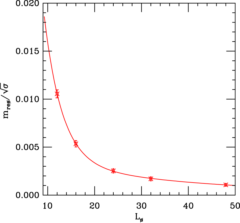
Figure 1: The residual mass normalized by the square root of the string tension ($\sigma$) as function of the $L_{s}$ for the Wilson gauge action at $\beta=6.0$ (results are from Blum et al. (2000)). The solid line is a fit to a double exponential. At large $L_{s}$ the decay is rather weak.

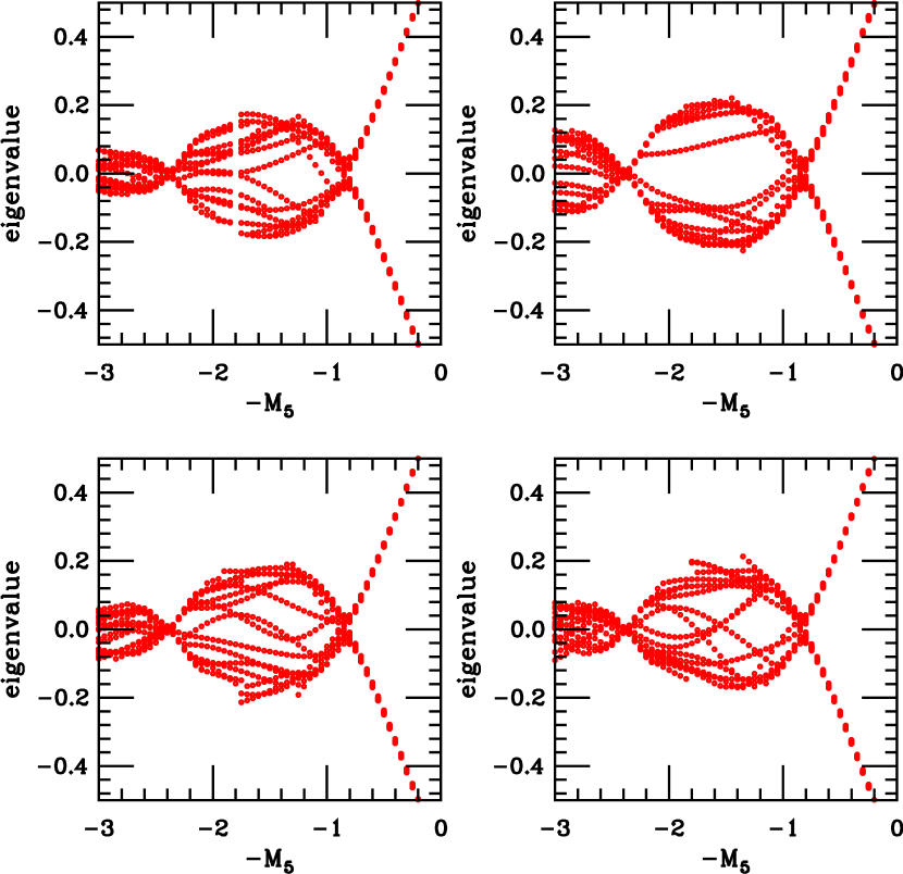
Figure 2: Spectral flows of the Hermitian Wilson Dirac operator $\gamma_{5}D_{W}$ for four typical gauge configurations generated with the Wilson gauge action at $\beta=6.0$. There are many crossings in the neighborhood of $M_{5}=1.8$ which induce explicit chiral symmetry breaking for domain wall fermions. The size of the would-be gap in the region of the five-dimensional fermion mass $M_{5}\approx 1.8$ is also relatively small compared to the obvious gap above the critical Wilson mass $M_{5}\approx 0.8$. Both effects enhance mixing of the light domain wall fermion modes and hence the value of the $m_{res}$.

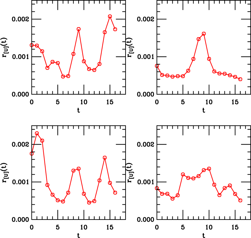
Figure 3: The ratio of Eq. 13 for four Wilson gauge configurations. The bare quark mass is $0.02$ and $M_{5}=1.8$. The configurations used are the same as those in Fig. 2 and the panels are in one to one correspondence with the panels in Fig. 2

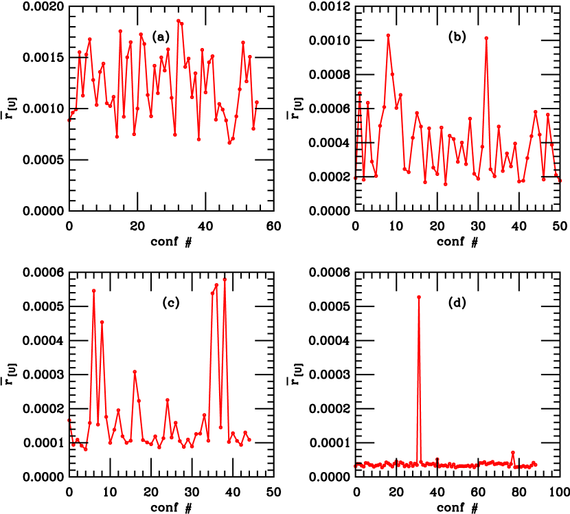
Figure 4: The quantity $\bar{r}_{[U]}$ defined in Eq. 14 vs. configuration number for (a) the Wilson gauge action at $\beta=6.0$, (b) the Symanzik gauge action at $\beta=8.4$, (c) the Iwasaki gauge action at $\beta=2.6$ , (d) and the DBW2 gauge action at $\beta=1.04$. All four cases correspond to $a^{-1}\approx 2\;{\rm GeV}$. The large spikes seen in the Wilson case are significantly reduced for the Iwasaki action and almost eliminated for the DBW2 action. These spikes corresponded to zero eigenvectors of $\gamma_{5}D_{W}$ and are a significant source of chiral symmetry breaking for domain wall fermions.

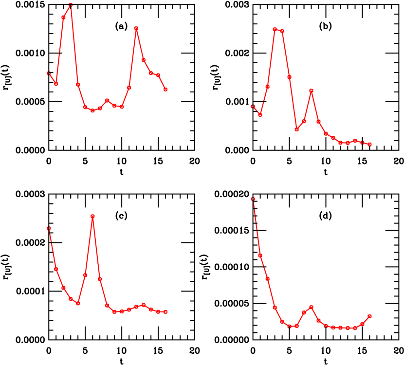
Figure 5: The ratio of Eq. 13 for a single configuration of (a) the Wilson gauge action at $\beta=6.0$, (b) the Symanzik gauge action at $\beta=8.4$, (c) the Iwasaki gauge action at $\beta=2.6$, (d) and the DBW2 gauge action at $\beta=1.04$. The spikes are quite localized in Euclidean time $t$. Examination of the eigenvectors of the (domain wall fermion or Wilson) Dirac operator confirms the zero modes are localized in space as well.

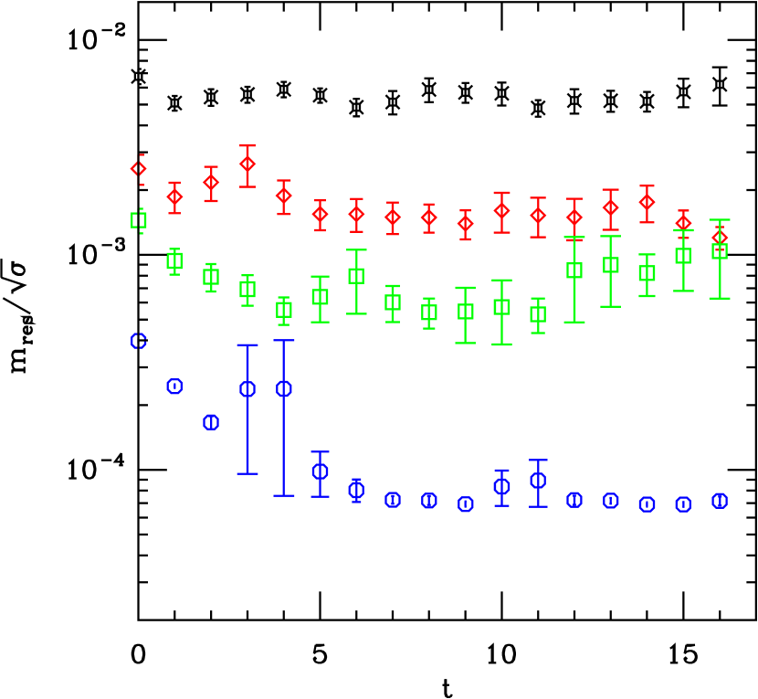
Figure 6: The ratio defined in Eq. 11 at $a^{-1}\approx 2$ GeV. The fancy squares correspond to the Wilson gauge action, the diamonds to Symanzik, the squares to Iwasaki, and the octagons to DBW2. The bare quark mass in all cases is 0.020 and $L_{s}=16$.

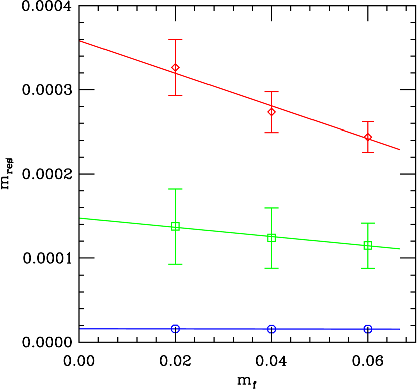
Figure 7: The residual mass at $a^{-1}\approx 2$ GeV as a function of the bare quark mass. The octagons correspond to DBW2, the squares to Iwasaki, and the diamonds to Symanzik. In each case $L_{s}=16$.

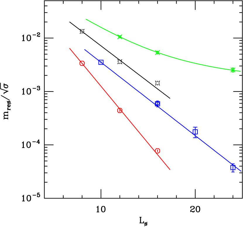
Figure 8: Dependence of the residual mass on the size of the 5th dimension at $a^{-1}\approx 2$ GeV. The octagons correspond to DBW2, the squares (CP-PACS Ali Khan et al. (2001)) and diamond (RBC Blum et al. (2000)) to Iwasaki, the bursts to Symanzik, and the fancy squares to Wilson. All but the Wilson action fit a simple exponential decay reasonably well. Note the Iwasaki results use different gauge field ensembles at each value of $L_{s}$. In the case of the Wilson action, the results are fit to a double exponential function.

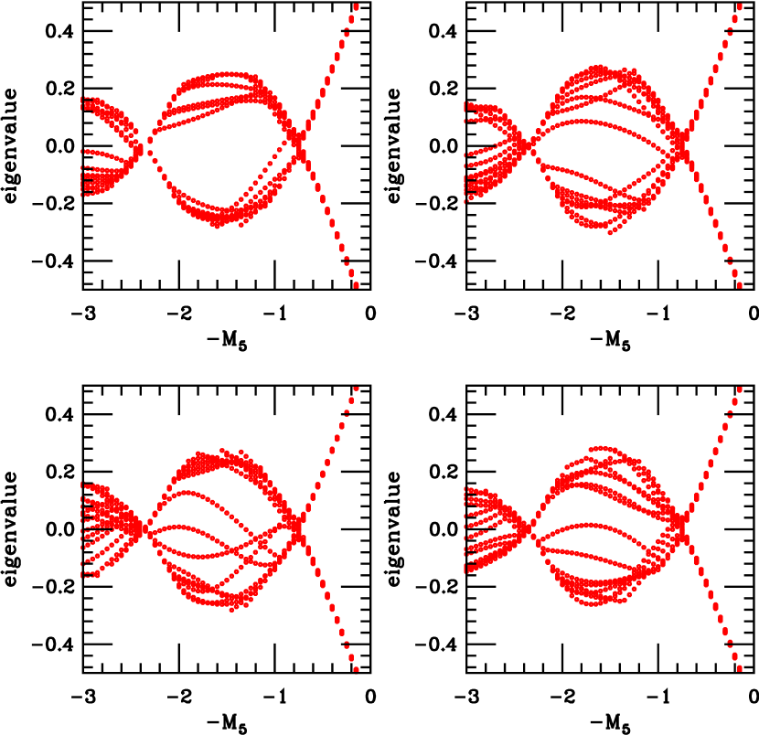
Figure 9: The same as Fig. 2, but for the Symanzik gauge action at $\beta=8.4$. The number of crossings in the neighborhood of $M_{5}=1.8$ appears slightly smaller and the would-be gap slightly larger than in the Wilson case.

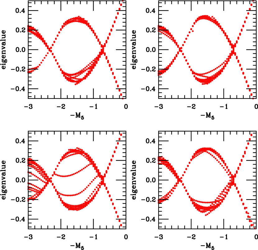
Figure 10: The same as Fig. 2, but for the Iwasaki gauge action at $\beta=2.6$. The number of crossings neighborhood of $M_{5}=1.8$ is significantly smaller and the gap clearly larger than in the Wilson case.

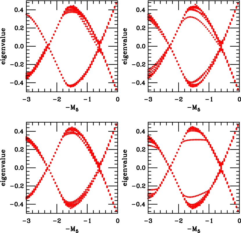
Figure 11: The same as Fig. 2, but for the DBW2 gauge action at $\beta=1.04$. There are no crossings neighborhood of $M_{5}=1.8$ and the gap is quite large, roughly comparable to the gap at the corresponding mass above the critical Wilson mass. Note that this is also true for the region beyond the next critical Wilson mass, $M_{5}\approx 2.3$, where the four flavor Wilson fermion doublers become light.

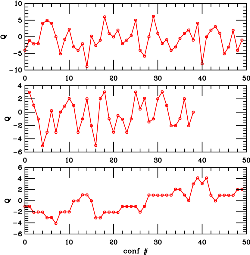
Figure 12: The configuration history of the topological charge $Q$. The configurations are separated by 1000 sweeps of Cabibo-Marinari pseudo-heatbath with a Kennedy-Pendleton accept/reject step. At the top is the Symanzik action with lattice size $16^{3}\times 32$ and coupling $\beta=8.4$. In the middle is the Iwasaki action with size $16^{4}$ and $\beta=2.6$. At the bottom is the DBW2 action with size $16^{3}\times 32$, and $\beta=1.04$. All cases correspond to roughly the same scale, $a^{-1}\approx 2$ GeV. The DWB2 action, which suppresses configurations with small instantons, shows a significant reduction of the tunneling between topological charge sectors.

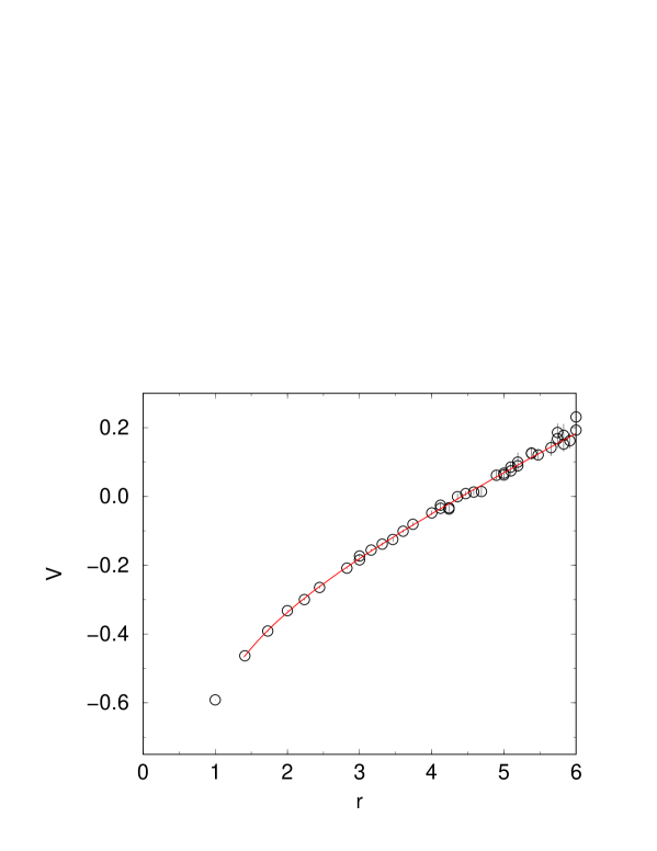
Figure 13: The heavy quark potential for DBW2, $\beta=0.87$. The solid line denotes the fit to Eq. 19 from which the string tension is determined.

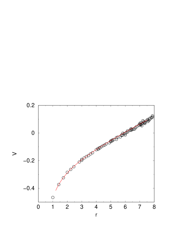
Figure 14: The same as Fig. 13 but for $\beta=1.04$.

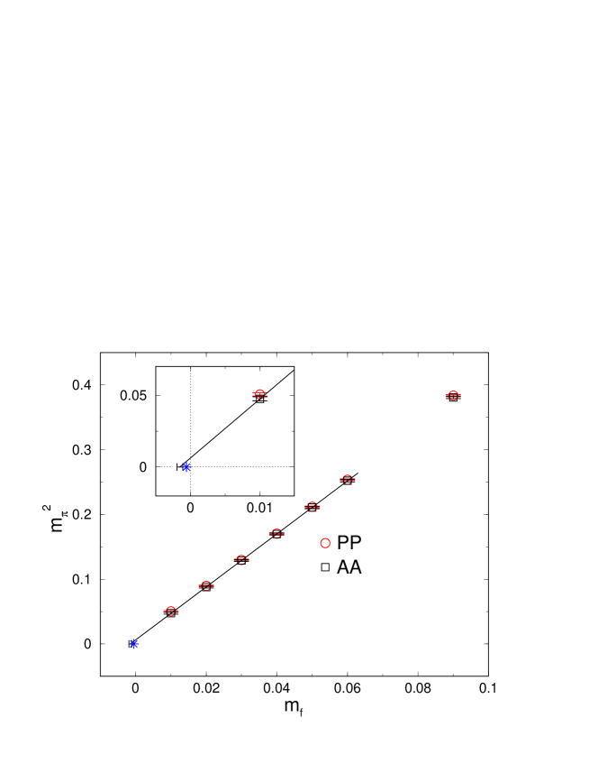
Figure 15: The quenched pion mass squared as a function of $m_{f}$ for $\beta=0.87$. Masses extracted from the pseudoscalar (PP) and axial vector (AA) correlation functions are shown. They agree quite well, except for the point at $m_{f}=0.01$ where there is a small difference outside of statistical errors. The physical volume is roughly $(2.4\,\,{\rm fm})^{3}$, so contamination from topological zero modes which can induce such splittings (see text) is suppressed. The line is a fit to a simple linear function. The extrapolation slightly overshoots the expected chiral limit point $m_{f}=-m_{\rm res}$ (see inset), suggesting a quenched chiral log.

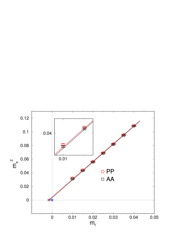
Figure 16: The same as Fig. 15, but for $\beta=1.04$. Here the physical volume is roughly $(1.6\,\,{\rm fm})^{3}$, so zero mode effects in the masses are visible, and the simple linear fit clearly overshoots the chiral limit point $m_{f}=-m_{\rm res}$.

Figure 17: Vector meson and baryon masses as functions of $m_{f}$ for $\beta=0.87$. Line is a linear fit to the data. The physical nucleon and $K^{*}$ mass are shown as solid points where $m_{\rho}$ is used to fix the scale.

Figure 18: Vector meson and baryon masses as functions of $m_{f}$ for $\beta=1.04$. The line is a linear fit to the data. The physical $K^{*}$ mass is also shown.

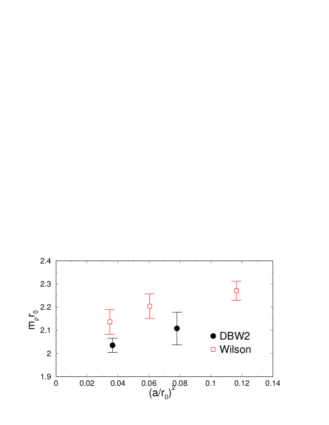
Figure 19: Scaling of the $\rho$ meson mass with the lattice spacing set by the Sommer parameter $r_{0}$. The Wilson data are from ref. Blum et al. (2000).

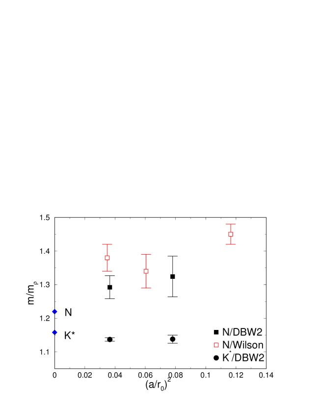
Figure 20: Scaling of the nucleon and $K^{*}$ masses with lattice spacing. The experimental mass of nucleon and $K^{*}$ are shown on the vertical axis. The Wilson data are from ref. Blum et al. (2000).

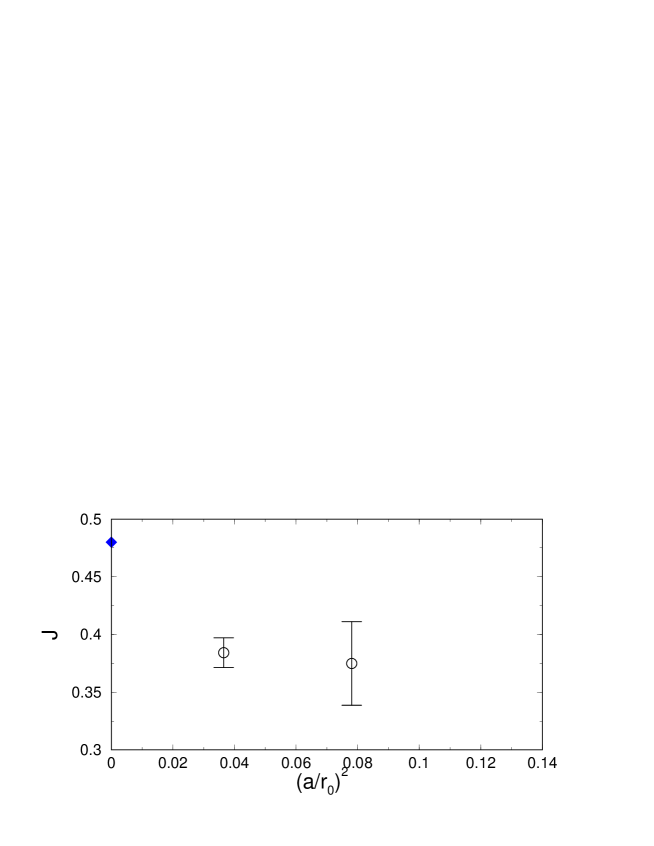
Figure 21: Scaling of the quenched J parameter with lattice spacing. The experimental point is shown on the vertical axis. The large discrepancy with experiment is due to quenching.

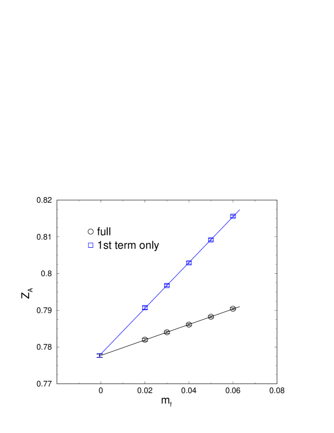
Figure 22: The local axial current renormalization factor as a function of $m_{f}$ for $\beta=0.87$. The lines correspond to fits to Eq. 26 (lower) and the first term only (upper). The difference arises from lattice spacing errors that are proportional to $m_{f}$.

Figure 23: The quenched pseudoscalar decay constant as a function of $m_{f}$ for $\beta=0.87$. The results from the two techniques described in the text agree quite well. The data are fit to simple linear functions, and extrapolated (pion) or interpolated (kaon) to the physical points (filled symbols).

Figure 24: The same as Fig. 23, but for $\beta=1.04$. Although the results agree within statistical errors, the agreement is not as good as that at $\beta=0.87$. Since the physical volume is significantly smaller in this case, we expect the difference is due to the presence of topological zero modes.

Figure 25: A scaling plot for the pion and kaon decay constants. The DBW2 results appear to preserve the good scaling that was observed with the use of the Wilson gauge action (data from Ref. Blum et al. (2000))

.