Generalized Parton Distributions and
the Spin Structure of the Nucleon

Abstract

Generalized parton distributions are a type of hadronic observables which has recently stimulated great interest among theorists and experimentalists alike. Introduced to delineate the spin structure of the nucleon, the orbital angular momentum of quarks in particular, the new distributions contain vast information about the internal structure of the nucleon, with the usual electromagnetic form factors and Feynman parton distributions as their special limits. While new perturbative QCD processes, such as deeply virtual Compton scattering and exclusive meson production, have been found to measure the distributions directly in experiments, lattice QCD offers a great promise to provide the first-principle calculations of these interesting observables.

Since the EMC experiment on polarized deep-inelastic scattering (DIS) on the proton in the late 1980s [1], QCD spin physics has evolved into one of the most active frontiers in hadron physics. The International Spin Physics Conference is held every other year with an average of 350 physicists participating in the meeting. The topics of the conference are often dominated by QCD spin physics. There are many experimental facilities around the world which have been playing a key role in spin physics research. For example, at CERN, following the EMC experiment there was SMC, and now the COMPASS experiment is on its way to take data [2]. At SLAC, a series of experiments were finished in the 1990s: E142, E143, E154, and E155. At DESY in Germany, the HERMES collaboration has taken data for a number of years, and new runnings have been planned (HERMES II). A summary of the finished experiments can be found in [3]. The spin physics at RHIC has just started, where 250 GeV polarized proton beams can be used to explore spin-dependent high-energy collisions [4]. Jefferson Lab in Virginia has a high intensity 6 GeV electron beam, and many experiments there involve polarized beams and targets. A plan has been made to upgrade the beam energy to 12 GeV. MIT-Bates delivered a polarized electron beam a few years ago, and a number of intereting low-energy experiments have been done which have an impact on spin physics.

There have been many important theoretical developments in spin physics as well. Perturbative QCD analysis of $g_{1}(x)$ and $g_{2}(x)$ structure functions of the nucleon has been carried out to two- and one-loop orders, respectively [5, 6]. The role of the axial anomaly in understanding the EMC results has been explored and debated [7]. A classification of the leading and higher-twist polarized quark and gluon distributions has been made [8]. QCD angular momentum and its role in high-energy scattering have been clarified [9]. The effects of parton transverse momentum in high-energy processes have been explored systematically [10]. Generalized parton distributions and deeply virtual Compton scattering are the main subject of this talk.

One of the most important goals in QCD spin physics is to understand the spin structure of the nucleon, i.e., how the nucleon spin is made from its fundamental constituents. Because nonperturbative QCD tools, such as lattice QCD, is still under development, we have relied, for many years, on model descriptions. In the naive SU(6) quark model, the three valence quarks move in the $s$-orbit, and the spin of the nucleon comes entirely from the coupling of the quark spins. There are a number of experimental evidences which seem to support this simple picture. For instance, the magnetic moment of the nucleon can be calculated in terms of the SU(6) wave function, and the ratio between the neutron and proton is [11]

$$\mu_{n}/\mu_{p}=-2/3\ .$$ (1)

The experimental data is $-0.68$, very close! Moreover, the $\Delta\rightarrow N\gamma$ transition can take place with both M1 and E2 electromagnetic multipoles. The quark model predicts that the E2 to M1 ratio is 0. Experimentally, the result is 1-3%, depending on how the background contribution is modelled. [However, recent results from the large $N_{c}$ QCD seem to indicate that these quark model predictions follow simply from the contracted SU(4) symmetry present in the large $N_{c}$ limit, independent of the detailed dynamics [12]].

This simple picture of the spin structure of the nucleon has been challenged by the polarized DIS data from CERN, SLAC and DESY [3]. In these experiments, the polarized quark distributions can be extracted:

$$\Delta q(x)=q_{+}(x)-q_{-}(x)\ ,$$ (2)

where $q_{\pm}(x)$ is the density of quarks with longitudinal momentum fraction $x$ and spin aligned (anti-aligned) to the spin of the nucleon. More precisely, the measured $g_{1}(x)$ structure function of the nucleon is related to the helicity distributions by

$$g_{1}(x)=\frac{1}{2}\sum_{f}e_{f}^{2}\Delta q_{f}(x)\ ,$$ (3)

where $f$ sums over light quark flavors. A summary of world data on the $g_{1}(x)$ structure functions for proton, neutron and deuteron is shown in Fig. 1.

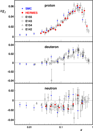
Figure 1: A compilation of world data on the $g_{1}(x)$ structure function of the proton, neutron (³He), and deuteron.

The operator production expansion (OPE) yields the deep-inelastic sum rule

$$\int^{1}_{0}g_{1}^{p}(x)dx=\frac{1}{18}(4\Delta u+\Delta d+\Delta s)\ ,$$ (4)

where $\Delta q$ is the fraction of the nucleon spin carried by the quark spin of flavor $q$. The total quark spin contribution to the proton spin

$$\int^{1}_{0}dx\sum_{q}\Delta q(x)=\Delta\Sigma=\Delta u+\Delta d+\Delta s\ ,$$ (5)

cannot be extracted from the DIS data alone. One must use the axial couplings $g_{A}$ determined from neutron and hyperon beta decay as well as the SU(3) flavor symmetry. An analysis of the world data to the next-to-leading order in perturbative QCD yields [3]

$$\Delta\Sigma(1~{}{\rm GeV}^{2})=0.2\pm 0.1\ .$$ (6)

Therefore, at least 70% of the proton spin resides in either the orbital motion of the quarks or gluons.

To understand the spin structure of the nucleon in the framework of QCD, one must start from the QCD angular momentum operator in its gauge-invariant form [13]:

$$\vec{J}_{\rm QCD}=\vec{J}_{q}+\vec{J}_{g}\,,$$ (7)

where

$$\vec{J}_{q} = \int d^{3}x~{}\vec{x}\times\vec{T}_{q}$$

$$= \int d^{3}x~{}\left[\psi^{\dagger}{\vec{\Sigma}\over 2}\psi+\psi^{\dagger}\vec{x}\times(-i\vec{D})\psi\right]\,,$$

$$\vec{J}_{g} = \int d^{3}x~{}\vec{x}\times(\vec{E}\times\vec{B})\,.$$ (8)

The quark and gluon parts of the angular momentum are generated from the quark and gluon momentum densities $\vec{T}_{q}$ and $\vec{E}\times\vec{B}$, respectively. $\vec{\Sigma}$ is the Dirac spin-matrix and the corresponding term is the quark spin contribution which we have discussed in the context of the polarized DIS. $\vec{D}=\vec{\nabla}-ig\vec{A}$ is the covariant derivative and the associated term is the gauge-invariant quark orbital contribution.

Using the above operator, one can easily construct a decomposition for the spin of the nucleon. Consider a nucleon moving in the $z$-direction, and in the helicity eigenstate $\lambda=1/2$. The total helicity can be calculated as an expectation value of $J_{z}$ in the nucleon state,

$${1\over 2}={1\over 2}\Delta\Sigma(\mu)+L_{q}(\mu)+J_{q}(\mu)\,,$$ (9)

where the three terms denote the matrix elements of three parts of the angular momentum operator in Eq. (8). The physical significance of each term is obvious, modulo the scale and scheme dependence indicated by $\mu$. The scale dependence in $\Sigma(\mu)$ is generated from the U(1) axial anomaly [7]. Note that the individual term in the above equation is independent of the momentum of the nucleon. In particular, it applies when the nucleon is travelling with the speed of light (the infinite momentum frame) [14].

The DIS data $\Delta\Sigma<\!<1$ indicates that the nucleon is much more complicated than the naive quark model depicts. At a phenomenological level, one may regard the quark model as an effective description but it is of little use to explain the DIS data if one does not know the relation between the QCD and constituent quarks. The challenge we have now is to find additional contributions to the nucleon spin in the context of the above decomposition.

From the definition, we see that $J_{q,g}$ are just the matrix elements of the moment of the energy-momentum tensor in a nucleon helicity state

$$J_{q,g}(\mu)=\left\langle P{1\over 2}\left|\int d^{3}x(\vec{x}\times\vec{T}_{q,g})^{z}\right|P{1\over 2}\right\rangle\,,$$ (10)

I will argue below that the matrix elements can be extracted from the form factors of the quark and gluon parts of the QCD energy-momentum tensor $T^{\mu\nu}_{q,g}$ in the nucleon state.

To motivate the linkage, let’s consider an analogous physics observable. In the electromagnetism, the magnetic moment is defined as a spatial moment of the current density

$$\vec{\mu}=\frac{1}{2}\int d^{3}x\vec{x}\times\vec{j}\ ,$$ (11)

If one knows the Dirac and Pauli form factors of the electromagnetic current, $F_{1}(Q^{2})$ and $F_{2}(Q^{2})$,

$$\langle P^{\prime}|j^{\mu}|P\rangle = \overline{U}(P^{\prime})\left[F_{1}(t)\gamma^{\mu}\right.$$ (12)

$$\left.+F_{2}(t)\frac{i\sigma^{\mu\nu}\Delta_{\nu}}{2M}\right]U(P)\ ,$$

where $t=(P-P^{\prime})^{2}$, and $\Delta=P-P^{\prime}$. The spin-flip form factor $\Delta G_{M}(t)=q(F_{1}(t)+F_{2}(t))$ yields the electric current distribution in the nucleon. From this, we can calculate the magnetic moment

$$\mu_{p}=G_{M}(0)=F_{1}(0)+F_{2}(0)\ ,$$ (13)

in units of $e\hbar/2Mc$.

Using Lorentz and discrete symmetries, it is easy to show that the symmetric and traceless part of the quark and gluon energy momentum tensors each supports three form factors,

$$\langle P^{\prime}|T_{q,g}^{\mu\nu}|P\rangle = \overline{U}(P^{\prime})\Big{[}A_{q,g}(t)\gamma^{(\mu}\overline{P}^{\nu)}$$ (14)

$$+B_{q,g}(t)\overline{P}^{(\mu}i\sigma^{\nu)\alpha}\Delta_{\alpha}/2M$$

$$+C_{q,g}(t)\Delta^{(\mu}\Delta^{\nu)}/M\Big{]}U(P)\,,$$

where $\overline{P}=(P+P^{\prime})/2$. Taking the forward limit of the $\mu=0$ component and integrating over 3-space, one finds that $A_{q,g}(0)$ give the momentum fractions of the nucleon carried by quarks and gluons (the momentum sum rule contraints $A_{q}(0)+A_{g}(0)=1$). On the other hand, substituting the above into the nucleon matrix element in Eq. (10), one finds [13]

$$J_{q,g}(\mu^{2})={1\over 2}\left[A_{q,g}(0,\mu^{2})+B_{q,g}(0,\mu^{2})\right]\,.$$ (15)

Therefore, the matrix elements of the energy-momentum tensor yield the fractions of the nucleon spin carried by quarks and gluons.

While a measurment of the gravitational form factors is impossible in the forseeable future, they can be extrated from QCD hard scattering. A process which was first identified is deeply virtual Compton scattering [13], in which a spacelike virtual photon created through lepton scattering, scatters off the nucleon target, yielding a final state of a real photon and a recoiled proton (see Fig. 2). When the virtual photon is in the Bjorken limit, the scattering process simplifies enormously: the single quark scattering dominates any other subprocesses and we have essentially a Compton scattering on a single quark. Compared with DIS in which the nucleon breaks into many fragments, DVCS in a sense is a non-invasive surgery.

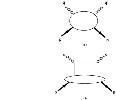
Figure 2: (a) Compton scattering on a nucleon; (b) Leading hand-bag contribution to DVCS.

The relation of the DVCS amplitude to the energy-momentum form factors can be seen as follows. The Compton scattering amplitude is a matrix element of the time-ordered product of the electromagnetic currents,

$$T^{\mu\nu}=i\int d^{4}ze^{\bar{q}\cdot z}\left\langle P^{\prime}\left|{\rm T}J^{\mu}\left(-{z\over 2}\right)J^{\nu}\left({z\over 2}\right)\right|P\right\rangle$$ (16)

where $\overline{q}=(q+q^{\prime})/2$. In the Bjorken limit, $-q^{2}$ and $P\cdot q\rightarrow\infty$ and their ratio remains finite, we can use the operator product expansion to approximate the current product,

$$TJ^{\mu}(\xi)J^{\nu}(0)=...+C^{\mu\nu\alpha\beta}(\xi^{2})\overline{\psi}\gamma_{\alpha}iD_{\beta}\psi+....$$ (17)

where $C^{\mu\nu\alpha\beta}$ is the coefficient function and other local operators have been omitted. Therefore, the DVCS amplitude contains the matrix element of the quark energy-momentum tensor [15]. The gluon contribution comes at the next-to-leading order. However, as the ellipses indicate, the DVCS amplitude contains much more information than just the energy-momentum tensor. It contains a whole new type of parton distributions.

To motivate the distributions, let us consider a form factor of a local current $\overline{\psi}\Gamma\psi(0)$. Its matrix element between the nucleon states $|P\rangle$ and $|P^{\prime}\rangle$ can be obtained (at least in the infinite momentum frame for a good component of the current) by annihilating a quark of momentum $\vec{k}$ at the spacetime point 0 and creating the same particle back at the same point with a new momentum $\vec{q}+\vec{k}$. On the other hand, the ordinary Feynman parton distribution $q(x)$ can be interpreted as a forward matrix element in the nucleon state in which a quark of momentum $xp^{\mu}$ is annihilated at point 0 and created back with the same momentum at a different spacetime point $\lambda n^{\mu}$, where $n$ is a light-cone vector $n^{2}=0$ conjugating to the nucleon momentum $p$.

The generalized parton distributions (GPDs) combine the spacetime structures of the above matrix elements. They are defined as an interference amplitude in which a quark is annihilated at spacetime point 0 with momentum $xp^{\mu}$, and created back at another point $\lambda n^{\mu}$ with a new momentum $xp^{\mu}+q^{\mu}$, yielding a recoiled nucleon. Therefore, the GPDs naturally include the elastic form factors and Feynman parton distributions in their kinematic limits. In fact, they contain much more information than the two traditional types of observables.

Technically, GPDs can be defined through the matrix elements of a bilocal light-cone operator [13, 16],

$${1\over 2}\int{d\lambda\over 2\pi}e^{i\lambda x}\left\langle P^{\prime}\left|\overline{\psi}_{q}\left(-{\lambda\over 2}n\right)\not\!n\right.\right.$$

$$\times\left.\left.{\cal P}e^{-ig\int^{-\lambda/2}_{\lambda/2}d\alpha~{}n\cdot A(\alpha n)}\psi_{q}\left({\lambda\over 2}n\right)\right|P\right\rangle$$

$$=H_{q}(x,\xi,t)~{}{1\over 2}\overline{U}(P^{\prime})\not\!nU(P)+E_{q}(x,\xi,t)~{}$$

$$~{}~{}~{}\times{1\over 2}\overline{U}(P^{\prime}){i\sigma^{\mu\nu}n_{\mu}\Delta_{\nu}\over 2M}U(P)\,.$$ (18)

The light-cone bilocal operator (or light-ray operator) arises frequently in hard scattering processes in which partons propagate along the light-cone. The parton distributions are most naturally defined in terms of the matrix elements of the bilocal operator. In this context, the Feynman $x$ is just the conjugating Fourier variable of the light-cone distance. The Lorentz structures in the second line in the above equation are independent and complete.

The GPD’s are more complicated than the Feynman parton distributions because of their dependence on the momentum transfer $\Delta$. As such, they contain two more scalar variables besides the Feynman variable $x$. The variable $t$ is the usual $t$-channel invariant which is always present in a form factor. The $\xi$ variable is a natural product of marrying the concepts of the Feynman distribution and form factor: The former requires the presence of a preferred momentum $p^{\mu}$ along which the partons are predominantly moving, and the latter requires a four-momentum transfer $\Delta$; $\xi$ is just a scalar product of the two momenta.

Since the quark and gluon energy-momentum tensors are just the twist-two, spin-two, parton helicity-independent operators, we immediately have the following sum rule from the off-forward distributions;

$$\int^{1}_{-1}dxx[H_{q}(x,\xi,t)+E_{q}(x,\xi,t)]$$ (19)

$$= A_{q}(t)+B_{q}(t)\,,$$

where the $\xi$ dependence, or $C_{q}(t)$ contamination, drops out. Extrapolating the sum rule to $t=0$, the total quark (and hence quark orbital) contribution to the nucleon spin is obtained. A similar sum rule exists for gluons. Thus a deep understanding of the spin structure of the nucleon may be achieved by measuring the GPDs from high energy experiments.

Recently, M. Burkardt has constructed an interpretation of GPD in the coordinate space [17]. Consider the nucleon state localized in the transverse plane at $r_{\perp}=0$,

$$|p^{+},r_{\perp}=0\rangle=N\int d^{2}p_{\perp}|p^{+},p_{\perp}\rangle\ ,$$ (20)

where $N$ is a normalization factor. Define a parton distribution $q(x,b_{\perp})$ which is the density of partons with longitudinal momentum $xp^{+}$ and the transverse distance $b_{\perp}$ in the state,

$$q(x,b_{\perp})=\int{d\lambda\over 4\pi}e^{ix\lambda}$$

$$~{}~{}~{}\times\langle p^{+},r_{\perp}|\overline{\psi}(0,b)\gamma^{+}\psi(\lambda n,b)|p^{+},r_{\perp}\rangle.$$ (21)

Then it can be shown that $q(x,b)$ is the Fourier transformation of $H(x,-\Delta_{\perp}^{2},\xi=0)$ with resprect to the transverse momentum transfer,

$$q(x,b)=\int d^{2}\Delta_{\perp}H(x,-\Delta^{2}_{\perp})e^{ib\cdot\Delta_{\perp}}\ .$$ (22)

Thus the GPDs provide the transverse location of the partons in the nucleon.

From the viewpoint of the low-energy nucleon structure, it is, perhaps, most interesting to consider GPDs as the generating functions for the form factors of the so-called twist-two operators. Recall that the matrix elements of the electromagnetic current in the same nucleon state are determined by symmetry, whereas those in the unequal momentum states define the (Dirac and Pauli) form factors which contain such interesting information as the charge radius and magnetic moment of the nucleon. The following tower of twist-two operators represents a generalization of the electromagnetic current

$${\cal O}^{\mu_{1}\cdots\mu_{n}}_{q}=\overline{\psi}_{q}i\stackrel{{\scriptstyle\leftrightarrow}}{{\cal D}}^{(\mu_{1}}\cdots i\stackrel{{\scriptstyle\leftrightarrow}}{{\cal D}}^{\mu_{n-1}}\gamma^{\mu_{n})}\psi_{q}\ ,$$ (23)

where all indices are symmetrized and traceless (indicated by $(\cdots)$) and $\stackrel{{\scriptstyle\leftrightarrow}}{{\cal D}}=(\stackrel{{\scriptstyle\rightarrow}}{{\cal D}}-\stackrel{{\scriptstyle\leftarrow}}{{\cal D}})/2.$ Technically, these operators transform as $(n/2,n/2)$ of the Lorentz group. They appear, as we have discussed before, in the operator production expansion of the two electromangetic currents. Thus, although these generalized currents do not couple directly to any known fundamental interactions, they can nonetheless be studied indirectly in hard scattering processes.

Since the operators for $n>1$ are not related to any symmetry in the QCD lagrangian, their matrix elements between the equal momentum states,

$$\langle P|{\cal O}^{\mu_{1}\cdots\mu_{n}}_{q}|P\rangle=2a_{n}(\mu)P^{(\mu_{1}}\cdots P^{\mu_{n})}\ ,$$ (24)

contain valuable dynamical information about the internal structure of the nucleon. The $\mu$ dependence of the above matrix elements signifies the dependence on renormalization scales and schemes. The quark distribution $q(x,\mu)$ introduced by Feynman has a simple connection to the above matrix elements:

$$\int^{1}_{-1}dxx^{n-1}q(x,\mu)=a_{n}(\mu)\ ,$$ (25)

where $q(x,\mu)$ is chosen to have support in $(-1,1)$. For $x>0$, $q(x,\mu)$ is the density of quarks which carry the $x$ fraction of the parent nucleon momentum. The density of antiquarks is customarily denoted as $\bar{q}(x,\mu)$, which in the above notation is $-q(-x,\mu)$.

Just like the form factors of the electromagnetic current, additional information about the nucleon structure can be found in the form factors of the twist-two operators when the matrix elements are taken between the states of unequal momenta. Using Lorentz symmetry and parity and time reversal invariance, one can write down all possible form factors of the spin-$n$ operator [18, 19, 20]

$$\langle P^{\prime}|O^{\mu_{1}\cdots\mu_{n}}_{q}|P\rangle$$

$$={\overline{U}}(P^{\prime})\gamma^{(\mu_{1}}U(P)$$

$$\times\sum_{i=0}^{[{n-1\over 2}]}A_{qn,2i}(t)\Delta^{\mu_{2}}\cdots\Delta^{\mu_{2i+1}}\overline{P}^{\mu_{2i+2}}\cdots\overline{P}^{\mu_{n})}$$

$$+~{}{\overline{U}}(P^{\prime}){\sigma^{(\mu_{1}\alpha}i\Delta_{\alpha}\over 2M}U(P)$$

$$\times\sum_{i=0}^{[{n-1\over 2}]}B_{qn,2i}(t)\Delta^{\mu_{2}}\cdots\Delta^{\mu_{2i+1}}\overline{P}^{\mu_{2i+2}}\cdots\overline{P}^{\mu_{n})}$$

$$+~{}C_{qn}(t)~{}{\rm Mod}(n+1,2)~{}{1\over M}\bar{U}(P^{\prime})U(P)$$

$$\times\Delta^{(\mu_{1}}\cdots\Delta^{\mu_{n})}\ ,$$ (26)

where ${\overline{U}}(P^{\prime})$ and $U(P)$ are the Dirac spinors and ${\rm Mod}(n+1,2)$ is 1 when $n$ even, 0 when $n$ odd. For $n\geq 1$, even or odd, there are $n+1$ form factors. $C_{qn}(t)$ is present only when $n$ is even.

Like the forward matrix elements $a_{n}$, the above form factors define GPDs completely. Introduce a light-like vector $n^{\mu}$, which is conjugate to $\overline{P}$ in the sense that $\bar{P}\cdot n=1$. Write $\overline{P}=p+(\overline{M}^{2}/2)n$, where $\overline{M}^{2}=M^{2}-t/4$ and $p$ is another light-like vector. Contracting both sides of Eq. (26) with $n_{\mu_{1}}\cdots n_{\mu_{n}}$, we have

$$n_{\mu_{1}}\cdots n_{\mu_{n}}\langle P^{\prime}|O^{\mu_{1}\cdots\mu_{n}}_{q}|P\rangle$$

$$={\overline{U}}(P^{\prime})\not\!nU(P)H_{qn}(\xi,t)$$

$$+{\overline{U}}(P^{\prime}){\sigma^{\mu\alpha}n_{\mu}i\Delta_{\alpha}\over 2M}U(P)E_{qn}(\xi,t)\ ,$$ (27)

where

$$H_{qn}(\xi,t) = \sum_{i=0}^{[{n-1\over 2}]}A_{qn,2i}(t)(-2\xi)^{2i}$$

$$+{\rm Mod}(n+1,2)~{}C_{qn}(t)(-2\xi)^{n}\ ,$$

$$E_{qn}(\xi,t) = \sum_{i=0}^{[{n-1\over 2}]}B_{qn,2i}(t)(-2\xi)^{2i}$$ (28)

$$-{\rm Mod}(n+1,2)~{}C_{qn}(t)(-2\xi)^{n}\ .$$

Here we have defined a new variable $\xi=-n\cdot\Delta/2$. Clearly, the $\xi$ dependence of $H_{qn}$ and $E_{qn}$ helps to distinguish among the different form factors of the same operator. Now the moments of $H(x,\xi,t)$ and $E(x,\xi,t)$ are simply

$$\int^{1}_{-1}dxx^{n-1}E_{q}(x,\xi,t) = E_{qn}(\xi,t)\ ,$$

$$\int^{1}_{-1}dxx^{n-1}H_{q}(x,\xi,t) = H_{qn}(\xi,t)\ .$$ (29)

Since all form factors are real, the new distributions are consequently real. Moreover, because of time-reversal and hermiticity, they are even functions of $\xi$.

The Compton amplitude can be expressed in terms of the GPDs. In the leading order,

$$T^{\mu\nu}=g^{\mu\nu}_{\perp}\int^{1}_{-1}dx\left({1\over x-\xi+i\epsilon}+{1\over x+\xi-i\epsilon}\right)$$

$$\times\sum_{q}e_{q}^{2}F_{q}(x,\xi,t,Q^{2})$$

$$+i\epsilon^{\mu\nu\alpha\beta}p_{\alpha}n_{\beta}\int^{1}_{-1}dx\left({1\over x-\xi+i\epsilon}-{1\over x+\xi-i\epsilon}\right)$$

$$\times\sum_{q}e_{q}^{2}\tilde{F}_{q}(x,\xi,t,Q^{2})\,,$$ (30)

where $n$ and $p$ are the conjugate light-cone vectors defined according to the collinear direction of $\overline{P}$, and $g^{\mu\nu}_{\perp}$ is the metric tensor in the transverse space. $\xi$ is related to the Bjorken variable $x_{B}=-q^{2}/(2P\cdot q)$ by $x_{B}=2\xi/(1+\xi)$. In addition to DVCS, the electromagnetic radiation from the scattering lepton, the so-called Bethe-Heitler process, also produces the same final state (background).

The first evidence for DVCS was seen by H1 and Zeus collaborations at the HERA collider, DESY [21, 22]. In Fig. 3, we have shown the differential cross section for $e^{+}p\rightarrow e^{+}\gamma p$ as a function of $Q^{2}$ from H1. The hatched histogram shows the contribution of the Bethe-Heitler process. There is a clear access of events above the background.

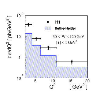
Figure 3: Cross section measurements for the $\gamma^{*}p\rightarrow\gamma p$ DVCS process as a function of $Q^{2}$ [22].

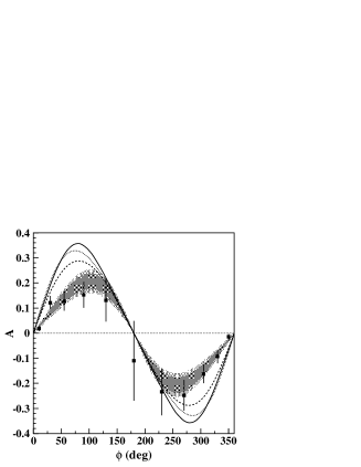
Figure 4: Single spin asymmetries measured by the CLAS collaboration which is sensitive to the inteference between Bethe-Heitler and DVCS processes.

At low-energy facilities such as JLab, the Bether-Heitler process overwhelms the cross section. In this case, one can isolate the interference contribution from the Bethe-Heitler and DVCS processes. Shown in Fig. 4 is the single beam spin asymmetry measured by CLAS as a function of the angle between the virtual and outgoing photons [23]. A similar data exist from the HERMES collaboration [24]. More experiments on DVCS will be done in the future at HERA, CERN, and Jefferson Lab.

An all-order proof of the DVCS factorization was discussed in [25] and in [15, 26]. Factorization concerns separation of soft physics at the scale of hadron masses and perturbative physics at the scale of probe in the DVCS amplitude. This can be done at the same level as for inclusive DIS. Therefore experimental cross section can be used to directly extract GPDs. This is nontrivial beause the final photon here is on-shell. Technically, it amounts to showing all soft physics either can be absorbed into the GPDs, which are nonperturbative anyway, or are down by powers of $1/Q^{2}$. The factorization result can be formulated in terms of an operator product expansion familiar in the field theory textbooks.

The next-to-leading order corrections to DVCS are important for a precision extraction of GPDs and for an estimate of scaling violation. The complete result is now known. The one-loop corrections to DVCS have first been studied by Osborne and Ji [15], and also by Belitsky and Mueller [27]. Two-loop anomalous dimensions were obtained by Belitsky and Muller [28]. It is the same as that for inclusive DIS except for the non-diagonal contribution which can be determined by the one-loop conformal anomaly. Classical chromodynamics is invariant under comformal symmetry which is broken by quantum mechanical effects. Because of this, an operator can acquire a scaling dimension under the spatial conformal transformation (conformal anomaly). The size for the NLO corrections has been estimated in [29].

The leading higher-twist contribution to DVCS comes from twist-three longitudinal photon scattering. In the interference amplitude, the imaginary part has a characteristic $\sin 2\phi$ and real part $\cos 2\phi$ dependence. The contribution can be estimated in the so-called Wilczek-Wendzura approximation (neglecting dynamical higher-twist effects). Belitsky, Mueller, and Kirchner et al. [32] found that the correction to the single spin asymmetry from the beam polarization is about 6%, and from the target polarization the correction is about 9%. For the spin-averaged cross section it is 17%, and 3% for the double spin asymmetry.

DVCS can be generalized to the case of exclusive production of mesons [30]. Collins, Frankfurt and Strikman have shown that the deep-exclusive meson production is factorizable to all orders in perturbation theory [31]. The vector meson production entails a rich spin and flavor structure. For example, the vector meson production is sensitive to quark helicity-independent distributions, whereas the pseudo-scalar mesons are sensitive to quark helicity-dependent distributions. The next-to-leading order perturbative QCD correction for pseudo-scalar meson production has first been calculated by Belitsky and Mueller [32]. Meson production may be easier to detect; however, it has a twist suppression, $1/Q^{2}$. In addition, the theoretical cross section depends on the unknown light-cone meson wave function. Recently, it has been found that a quantity very sensitive to the quark angular momentum is the target transverse spin asymmetry for vector meson production [33].The asymmetry comes from the interference of two DVCS amplitudes and is linear in the $E(x,\xi,t)$ distribution. Since the asymmetry involves the ratio, it is insensitive to the next-to-leading order and higher-twist effects. The vector meson final state allows separation of different quark flavors. For example, the $\rho^{0}$ production is sensitive to the combination $2J_{u}+J_{d}$, the $\omega$ meson is sensitive to $2J_{u}-J_{d}$, and finally the $\rho^{+}$ meson is sensitive to the $J_{u}-J_{d}$ combination.

To summarize, the recently discovered generalized parton distributions are a new type of nucleon observables which contain rich information about the internal structure of the nucleon. Many experiments have been planned to measure the distributions. Lattice QCD will be a unique theoretical tool to calculate the distribution from the first principles [34].

References

- [1] J. Ashman et al., Nucl. Phys. B 328, 1 (1989).
- [2] CERN/SPSLC 96-14 (1996); http://www.compass.cern.ch/
- [3] B. W. Filippone and X. Ji, Adv. in Nucl. Phys. Vol. 26, 1-88 (2001).
- [4] G. Bunce, N. Saito, J. Soffer, and W. Vogelsang, Ann. Rev. Nucl. Part. Sci. 50, 525 (2000).
- [5] J. Kodaira, S. Matsuda, K. Sasaki and T. Uematsu, Nucl. Phys. B 159, 99 (1979). E. B. Zijlstra and W. L. van Neerven, Nucl. Phys. B 417, 61 (1994) [Erratum-ibid. B 426, 245 (1994)]; M. Stratmann, A. Weber and W. Vogelsang, Phys. Rev. D 53, 138 (1996) [arXiv:hep-ph/9509236].
- [6] X. Ji, W. Lu, J. Osborne and X. T. Song, Phys. Rev. D 62, 094016 (2000); A. V. Belitsky, X. Ji, W. Lu and J. Osborne, Phys. Rev. D 63, 094012 (2001); V. M. Braun, G. P. Korchemsky and A. N. Manashov, Nucl. Phys. B 597, 370 (2001) [arXiv:hep-ph/0010128]; X. Ji and J. Osborne, Nucl. Phys. B 608, 235 (2001)
- [7] G. Altarelli and G. G. Ross, Phys. Lett. B 212, 391 (1988); R. D. Carlitz, J. C. Collins and A. H. Mueller, Phys. Lett. B 214, 229 (1988);
- [8] R. L. Jaffe and X. D. Ji, Phys. Rev. Lett. 67, 552 (1991); R. L. Jaffe and X. D. Ji, Nucl. Phys. B 375, 527 (1992).
- [9] R. L. Jaffe and A. Manohar, Nucl. Phys. B 337, 509 (1990); X. Ji, J. Tang and P. Hoodbhoy, Phys. Rev. Lett. 76, 740 (1996); P. Hagler and A. Schafer, Phys. Lett. B 430, 179 (1998); S. V. Bashinsky and R. L. Jaffe, Nucl. Phys. B 536, 303 (1998); P. Hoodbhoy, X. Ji and W. Lu, Phys. Rev. D 59, 014013 (1999); P. Hoodbhoy, X. Ji and W. Lu, Phys. Rev. D 59, 074010 (1999).
- [10] P. J. Mulders and R. D. Tangerman, Nucl. Phys. B 461, 197 (1996) [Erratum-ibid. B 484, 538 (1997)] [arXiv:hep-ph/9510301].
- [11] M. A. Beg, B. W. Lee and A. Pais, Phys. Rev. Lett. 13, 514 (1964).
- [12] E. Jenkins, Ann. Rev. Nucl. Part. Sci. 48, 81 (1998); R. F. Dashen and A. V. Manohar, Phys. Lett. B 315, 425 (1993); E. Jenkins, Phys. Lett. B 315, 431 (1993); R. F. Dashen, E. Jenkins and A. V. Manohar, Phys. Rev. D 49, 4713 (1994) [Erratum-ibid. D 51, 2489 (1995)]; E. Jenkins, X. Ji and A. V. Manohar, arXiv:hep-ph/0207092.
- [13] X. Ji, Phys. Rev. Lett. 78, 610 (1997); Phys. Rev. D 55, 7114 (1997).
- [14] X. Ji, Phys. Rev. D 58, 056003 (1998).
- [15] X. Ji and J. Osborne, Phys. Rev. D 58, 094018 (1998).
- [16] D. Müller, D. Robaschik, B. Geyer, F. M. Dittes, J. Horejsi, Fortsch. Phys. 42, 101 (1994).
- [17] M. Burkardt, Phys. Rev. D 62, 071503 (2000); hep-ph/0207047.
- [18] X. Ji, W. Melnitchouk and X. Song, Phys. Rev. D 56, 5511 (1997) [arXiv:hep-ph/9702379].
- [19] X. Ji, J. Phys. G 24, 1181 (1998) [arXiv:hep-ph/9807358].
- [20] X. Ji and R. F. Lebed,Phys. Rev. D 63, 076005 (2001)[arXiv:hep-ph/0012160].
- [21] P. R. Saull [ZEUS Collaboration], arXiv:hep-ex/0003030.
- [22] C. Adloff et al. [H1 Collaboration], Phys. Lett. B 517, 47 (2001).
- [23] S. Stepanyan et al. [CLAS Collaboration], measurements,” Phys. Rev. Lett. 87, 182002 (2001)
- [24] A. Airapetian et al. [HERMES Collaboration], Phys. Rev. Lett. 87, 182001 (2001)
- [25] A. V. Radyushkin, Phys. Rev. D 56, 5524 (1997).
- [26] J. C. Collins and A. Freund, Phys. Rev. D 59, 074009 (1999).
- [27] A. V. Belitsky and D. Müller, Phys. Lett. B 417, 129 (1998).
- [28] A. V. Belitsky and D. Müller, Nucl. Phys. B 537, 397 (1999).
- [29] A. V. Belitsky, D. Müller, and A. Kirchner, Nucl. Phys. B 629, 323 (2002).
- [30] A. V. Radyushkin, Phys. Lett. B 385, 333 (1996).
- [31] J. C. Collins, F. Frankfurt, and M. Strikman, Phys. Rev. D 56, 2982 (1997).
- [32] A. V. Belitsky and D. Müller, Phys. Lett. B 493 (2000) 341.
- [33] K. Goeke, M. V. Polyakov, and M. Vanderhaeghen, Prog. Part. Nucl. Phys. 47, 401 (2001).
- [34] N. Mathur, S. J. Dong, K. F. Liu, L. Mankiewicz and N. C. Mukhopadhyay, Phys. Rev. D 62, 114504 (2000); V. Gadiyak, X. Ji and C. W. Jung, Phys. Rev. D 65, 094510 (2002) [arXiv:hep-lat/0112040].