Heavy-light mesons with staggered light quarks

Abstract

We demonstrate the viability of improved staggered light quarks in studies of heavy-light systems. Our method for constructing heavy-light operators exploits the close relation between naive and staggered fermions. The new approach is tested on quenched configurations using several staggered actions combined with nonrelativistic heavy quarks. Exploratory calculations of the $B_{s}$ meson kinetic mass, the hyperfine and $1P-1S$ splittings in $B_{s}$, and the decay constant $f_{B_{s}}$ are presented and compared to previous quenched lattice studies. An important technical detail, Bayesian curve-fitting, is discussed at length.

I Introduction

Precise calculations of hadronic matrix elements are important ingredients in the quest to constrain the flavor-mixing parameters of the Standard Model, the Cabibbo-Kobayashi-Maskawa matrix elements $V_{ff^{\prime}}$. For example, the main theoretical input in extracting the ratio $|V_{td}/V_{ts}|$ involves a combination of the decay constants, $f_{B}$ and $f_{B_{s}}$, which parameterize leptonic $B$ and $B_{s}$ decays, and of the neutral $B$ and $B_{s}$ mixing parameters, $B_{B}$ and $B_{B_{s}}$. Uncertainties in these quantities, or more specifically in the combination $\xi\equiv(f_{B_{s}}/f_{B})\sqrt{B_{B_{s}}/B_{B}}$, currently restrict our ability to carry out stringent consistency checks of the Standard Model (e.g. see Ligeti (2001)). If these theoretical errors could be reduced by a factor of 2 or more the impact would be immediate and far-reaching. Similarly, high precision theoretical calculations of form factors governing $B\to D\ell\bar{\nu}$ and $B\to\pi\ell\bar{\nu}$ decays are crucial to determinations of $|V_{cb}|$ and $|V_{ub}|$, respectively.

Monte Carlo simulation of QCD on a lattice will ultimately provide the most accurate theoretical determinations of mixing parameters, decay constants, and form factors since lattice QCD is one of the few systematically improvable approaches to QCD. Understanding and removing systematic uncertainties in lattice calculations, however, is arduous and complicated, and much of the effort in lattice gauge theory over the past decade has focused on this task. One very promising outcome of all this activity is the emergence of improved staggered actions for light quarks combined with highly improved glue actions. The MILC collaboration, for instance, works with the “AsqTad” quark action which is free from the leading discretization errors, including those arising from the breaking of the fermion doubling symmetry, so that the action is accurate up to $O\left(\alpha_{s}a^{2}\right)$ errors. They employ the one-loop Symanzik improved glue action with errors coming in only at $O\left(\alpha_{s}^{2}a^{2}\right)$. Staggered actions have an exact chiral symmetry at zero mass and are much cheaper to simulate than Wilson-type quark actions, so it has been possible for the MILC collaboration to carry out unquenched simulations with much smaller dynamical quark masses than has been attempted in the past. They are now starting to obtain impressive results for light hadron spectroscopy and light meson decay constants Bernard et al. (2001, 2002).

In this article we demonstrate that improved staggered quarks can also be used very effectively to simulate the light quark in heavy-light systems such as in $B$-physics. The past decade has seen significant progress in our ability to simulate heavy quarks accurately (the commonly used NRQCD action, for instance, has errors coming in at $O\left(\alpha_{s}a^{2}\right)$ and $O\left(\alpha_{s}\Lambda_{\rm QCD}/M\right)$, and work is underway to remove the latter). On the other hand, only Wilson-type actions have been used for the valence light quarks in heavy-light mesons, baryons, and electroweak currents, making it difficult to go much below $m_{\rm strange}/2$ in the light quark mass due to the necessary computational expense. Consequently, the extrapolation of simulation results to the chiral limit leads to the dominant systematic error in studies of $B$ and $D$ mesons (aside from quenching uncertainties). Furthermore the leading discretization errors in heavy-light simulations come from the light quark sector since Wilson-type actions have worse finite lattice spacing errors than improved glue, improved staggered, or NRQCD actions. This situation motivated us to initiate a new approach to heavy-light simulations, namely the use of improved staggered light quarks combined with nonrelativistic heavy quarks. Our approach can trivially be modified to use a Wilson-like action for the heavy quark instead of NRQCD. The goal is to simulate $B$ physics at much smaller light quark masses than has been possible in the past and significantly reduce chiral extrapolation errors in decay constants, form factors and mixing parameters. Work toward this goal has already started on the MILC dynamical configurations Wingate et al. (2002). It is important, however, to first establish that we understand how to combine staggered light and NRQCD or Wilson heavy fermions to form heavy-light operators, that we are able to carry out sophisticated fits to simulation data and extract physics reliably, and that these methods produce results in agreement with well-established results. It is for the last reason that this article focuses on the $B_{s}$ system on quenched lattices, where methods existing in the literature provide a solid basis for comparison. We present results for $B_{s}$ meson kinetic masses, some level splittings, and the decay constant $f_{B_{s}}$ as evidence that our approach is working. For quick reference, we summarize the results of our finest isotropic lattice in Table 1. Note that several systematic uncertainties remain, notably the error from determining the spacing on quenched lattices and discretization errors from using coarse lattices with the present level of improvement. Therefore, the results presented in this paper are useful for comparison to similar lattice calculations, but they are not appropriate for inclusion in phenomenological analyses. Having established this method as a promising approach, work is now underway on unquenched lattices to remove or reduce the systematic uncertainties and obtain state-of-the-art lattice QCD results.

In the next section we introduce and describe the formalism for combining staggered light quarks with heavy quark fields to form bilinear operators that create heavy-light mesons or represent heavy-light currents. A significant simplification comes about from recognizing the equivalence of staggered and naive fermions and writing down bilinears in terms of the latter. This will be explained thoroughly below. In Section III we give simulation details starting with a description of the glue, heavy quark, and light quark actions and then a discussion of our constrained fitting methods based on Bayesian statistics. Section IV gives results for heavy-light spectroscopy, including kinetic masses and a calculation of the $B_{s}$ meson decay constant $f_{B_{s}}$. Three appendices contain details regarding the theory, notation, and fitting techniques, respectively.

II Formalism

In this section we describe how to combine naive/staggered light quarks with heavy quarks to form heavy-light meson and electroweak current operators. We adhere to the recently introduced practice of calling the doubler degrees of freedom “tastes” rather than “flavors” Bernard and Lepage (see also Aubin et al. (2002)). We will be guided by the following properties of naive/staggered actions.

1. Up to overall normalization factors, there is no difference between using naive or staggered valence quarks in meson creation or current operators. Since naive fermions are easier to interpret and to handle theoretically, we will construct our heavy-light bilinears using naive fermion fields rather than staggered fields.

2. Any correlator involving naive fermion propagators can be rewritten in terms of staggered propagators. Since staggered propagators are cheaper to calculate numerically, when it comes to actual simulations we will always work with expressions that have been converted to the staggered fermion language and involve only staggered (and heavy) quark propagators.

3. The taste content of naive/staggered actions can be determined either in the coordinate or the momentum space basis. For heavy-light physics and for perturbation theory we find the momentum space interpretation to be more useful.

We start by reviewing naive fermions and the identification of different tastes in momentum space. We will then explore the taste content of $B$ mesons that appear when naive fermions are combined with heavy fermions. We assume that the heavy quark action has no doublers, as in NRQCD, or that doublers have been given masses of order the cutoff via a Wilson term, as in the Fermilab approach El-Khadra et al. (1997). Heavy-light systems are much simpler than light-light systems since the heavy quark suppresses the taste-changing processes of the naive/staggered quark.

II.1 The free naive quark action

Most of our discussion in this section will be for free unimproved naive fermions. Taste identification and relevant symmetries survive the inclusion of gauge interactions and of the $O\left(a^{2}\right)$ improvement terms incorporated into the action that we actually use in our simulations (see next section for a description of the full action). The free unimproved naive fermion action is given by,

$${\cal S}_{0}=a^{4}\sum_{x}\left\{\overline{\Psi}(x)\,\left[\sum_{\mu}\gamma_{\mu}{\frac{1}{a}}\nabla_{\mu}\;+\;m\right]\Psi(x)\right\},$$ (1)

with

$$\nabla_{\mu}\Psi(x)={\mbox{$\frac{1}{2}$}}\,[\Psi(x+a_{\mu})-\Psi(x-a_{\mu})].$$ (2)

We work with hermitian Euclidean $\gamma$-matrices obeying $\{\gamma_{\mu},\gamma_{\nu}\}=2\delta_{\mu\nu}$. It is well-known that the action (1) describes a theory with 16 tastes of Dirac fermions and that it has a set of discrete “doubling” symmetries,

$$\Psi(x) \rightarrow e^{ix\cdot\pi_{g}}M_{g}\Psi(x)$$

$$\overline{\Psi}(x) \rightarrow e^{ix\cdot\pi_{g}}\overline{\Psi}(x)M_{g}^{\dagger}\,.$$ (3)

$g$ is an element of $G$, the set of ordered lists of up to 4 indices,

$$G=\left\{g:g=(\mu_{1},\mu_{2},\ldots),\;\mu_{1}<\mu_{2}<\ldots\right\}\;;$$ (4)

e.g. $(2)$, $(0,3)$, and $(0,1,2,3)$ are elements of $G$, as is the empty set $\emptyset$. The corners of the Brillouin zone are denoted by the 4-vector $\pi_{g}$ such that

$$\left(\pi_{g}\right)_{\mu}=\cases{\frac{\pi}{a}\qquad\mu\in g,\cr 0\qquad{\rm otherwise}.\cr}$$ (5)

The $M_{g}$ are transformation matrices

$$M_{g}=\prod_{\mu\in g}~{}M_{\mu}$$ (6)

with

$$M_{\mu}=i\gamma_{5}\gamma_{\mu}.$$ (7)

An illustrative way to reduce the taste degeneracy of the naive action is to diagonalize the action in spin space. Let $\overline{\Phi}(x)$ and $\Phi(x)$ be a new set of 4-component spinor fields related to the original $\overline{\Psi}(x)$ and $\Psi(x)$ fields via the Kawamoto-Smit Kawamoto and Smit (1981) transformation.

$$\Psi(x)=\Omega(x)\,\Phi(x)\qquad\qquad\overline{\Psi}(x)=\overline{\Phi}(x)\,\Omega(x)^{\dagger}$$ (8)

with

$$\Omega(x)=\prod^{3}_{\mu=0}(\gamma_{\mu})^{x_{\mu}/a}\,.$$ (9)

In terms of these new fields the naive fermion action takes on a spin-diagonal form,

$${\cal S}_{0}\rightarrow{\cal S}_{\Phi}=a^{4}\sum_{x}\left\{\overline{\Phi}(x)\,\left[\sum_{\mu}\eta_{\mu}(x){\frac{1}{a}}\nabla_{\mu}\;+\;m\right]\Phi(x)\right\},$$ (10)

where

$$\eta_{\mu}(x)=(-1)^{(x_{0}+\ldots+x_{\mu-1})/a}\,.$$ (11)

Staggered fermions reduce the taste-degeneracy from 16-fold to 4-fold. The spin-diagonal form of Eq. (10) tells us it should be possible to do so, since each spin component of $\Phi(x)$ is independent of the other components. One way to proceed is to define 1-component fields $\chi(x)$ through

$$\Phi(x)\equiv e(x)\chi(x)\,.$$ (12)

The c-number spinor $e(x)$ is usually chosen to be constant, and one ends up with the standard staggered fermion action for the fields $\chi(x)$. Reference Sharatchandra et al. (1981) goes through a more rigorous and general method for reducing the number of independent tastes from 16 to 4 which does not rely on first going through the Kawamoto-Smit transformation. They exploit the symmetry (II.1) to place constraints among the 16 different tastes so that only 4 of them remain as independent degrees of freedom. (See also Chodos and Healy (1977) which uses the Hamiltonian formalism .)

Equations (8) and (10) allow us to derive the simple but important relation between the naive propagator $G_{\Psi}(x;y)$ and the staggered propagator $G_{\chi}(x;y)$. One has,

$${\rm Eq.}~{}(\ref{spindiag})\quad \Longrightarrow \quad G_{\Psi}(x;y)\;\equiv\;\Omega(x)\;G_{\Phi}(x;y)\;\Omega(y)^{\dagger}$$ (13)

$${\rm Eq.}~{}(\ref{phiaction})\quad \Longrightarrow \quad G_{\Phi}(x;y)\;\equiv\;\hat{I}_{4}\;G_{\chi}(x;y)\,,$$ (14)

with $\hat{I}_{4}$ equal to a $4\times 4$ identity matrix in Dirac space. This leads to

$$G_{\Psi}(x;y)\;\equiv\;\Omega(x)\Omega^{\dagger}(y)\;\times\;G_{\chi}(x;y).$$ (15)

We use the identity (15) repeatedly in the present work to go from bilinears expressed in terms of naive fermion fields to correlators written in terms of staggered propagators. It can also be used to rederive familiar staggered correlators (e.g. for pions or rhos) starting from simple naive fermion bilinears. We emphasize that (15) is an exact relation even in the presence of gauge interactions; re-expressed as a relation between the inverse of the naive and staggered actions, respectively, for fixed gauge fields, it is valid configuration by configuration, and hence also for the fully interacting naive and staggered propagators. The relation (15) also holds for improved versions of naive/staggered actions.

Before going on to discuss heavy-light bilinears, we end this subsection on basic naive fermion properties by reviewing the momentum space identification of naive fermion tastes. We continue to use the notation of Sharatchandra et al. (1981). The momentum space spinors are given by,

$$\psi(k)=a^{4}\sum_{x}e^{-ik\cdot x}\Psi(x)\qquad,\qquad\overline{\psi}(k)=a^{4}\sum_{x}e^{ik\cdot x}\overline{\Psi}(x)$$ (16)

with the inverse relation given by

$$\Psi(x)=\int_{k,D}e^{ik\cdot x}\psi(k)\qquad,\qquad\overline{\Psi}(x)=\int_{k,D}e^{-ik\cdot x}\overline{\psi}(k).$$ (17)

We use the notation,

$$\int_{k,D}\equiv\int_{k\in D}\frac{d^{4}k}{(2\pi)^{4}}\qquad,\qquad\int_{k,D_{\emptyset}}\equiv\int_{k\in D_{\emptyset}}\frac{d^{4}k}{(2\pi)^{4}}$$ (18)

where $D$ denotes the full Brillouin zone, $-\frac{\pi}{a}\leq k_{\mu}<\frac{\pi}{a}$, and $D_{\emptyset}$ just the central region, $-\frac{\pi}{2a}\leq k_{\mu}<\frac{\pi}{2a}$. In terms of the momentum space spinors the free action (1) becomes

$${\cal S}_{0}=\int_{k,D}\overline{\psi}(k)\left[\sum_{\mu}i\gamma_{\mu}\frac{1}{a}\sin(k_{\mu}a)\;+\;m\right]\psi(k)$$ (19)

Using the 4-vectors $\pi_{g}$ this can be written as,

$${\cal S}_{0}=\sum_{g}\int_{k,D_{\emptyset}}\overline{\psi}(k+\pi_{g})\left[\sum_{\mu}i\gamma_{\mu}\frac{1}{a}\sin([k+\pi_{g}]_{\mu}a)\;+\;m\right]\psi(k+\pi_{g})$$ (20)

The next step is to define 16 new momentum space spinors $q^{g}(k)$ labeled by the elements $g$ of the set $G$ (4)

$$q^{g}(k)=M_{g}\psi(k+\pi_{g})\qquad,\qquad\overline{q}^{g}(k)=\overline{\psi}(k+\pi_{g})M_{g}^{\dagger}\,;$$ (21)

the matrices $M_{g}$ are those of (6). In terms of these new spinors, $q^{g}(k)$, and upon using the relation

$$M_{g}\gamma_{\mu}M_{g}^{\dagger}\,\sin([k+\pi_{g}]_{\mu}a)=\gamma_{\mu}\,\sin(k_{\mu}a),$$ (22)

the action ${\cal S}_{0}$ becomes

$${\cal S}_{0}=\sum_{g}\int_{k,D_{\emptyset}}\overline{q}^{g}(k)\left[\sum_{\mu}i\gamma_{\mu}\frac{1}{a}\sin(k_{\mu}a)\;+\;m\right]q^{g}(k).$$ (23)

Eq. (23) clearly describes an action for 16 “tastes” of Dirac fermions. The sum $\sum_{g}$ over the elements of the set $G$ can be interpreted as a sum over tastes. The doubling symmetry (II.1) which in momentum space becomes

$$\psi(k) \rightarrow M_{g}\psi(k+\pi_{g})$$

$$\overline{\psi}(k) \rightarrow \overline{\psi}(k+\pi_{g})M_{g}^{\dagger},$$ (24)

takes one $q^{g}(k)$ taste into another up to possible sign factors, $\epsilon_{g_{1},g_{2}}=\pm 1$, defined through $M_{g_{1}}M_{g_{2}}=\epsilon_{g_{1},g_{2}}M_{g_{1}g_{2}}$ (see Ref. Sharatchandra et al. (1981)).

II.2 Heavy-light bilinears

To discuss heavy-light bilinears we introduce heavy quark fields $\Psi_{H}$, which can stand for either heavy Wilson or nonrelativistic fermions (for the latter case we will use the notation $\Psi_{H}(x)\rightarrow Q(x)$ in later sections with $Q(x)$ a 4-component spinor with vanishing lower 2 components). The simplest interpolating operator one could write down for creating a $B$ meson with a heavy quark field $\overline{\Psi}_{H}(x)$ and a naive antiquark field $\Psi(x)$ is

$${\cal W}_{B}(x)=\overline{\Psi}_{H}(x)\gamma_{5}\Psi(x)\,.$$ (25)

Let us analyze ${\cal W}_{B}(x)$ in 3-dimensional momentum space. To do so we introduce the 3D Fourier transformed fields

$$\tilde{\psi}({\bf\bm{k}},t)=a^{3}\sum_{{\bf\bm{x}}}e^{-i{\bf\bm{k}}\cdot{\bf\bm{x}}}\;\Psi({\bf\bm{x}},t)\qquad,\qquad\overline{\tilde{\psi}}({\bf\bm{k}},t)=a^{3}\sum_{{\bf\bm{x}}}e^{i{\bf\bm{k}}\cdot{\bf\bm{x}}}\;\overline{\Psi}({\bf\bm{x}},t)$$ (26)

and similarly for the heavy fields $\Psi_{H}$. It is useful to introduce a subset $G_{s}\subset G$ that involves only spatial indices $\mu\rightarrow j=1,2,3$. The full set $G$ can be built up out of $g_{s}$ and $g_{t}g_{s}$ with $g_{s}\in G_{s}$ and $g_{t}$ corresponding to $\mu=0$ (and $M_{g_{t}}=i\gamma_{5}\gamma_{0}$). In analogy with (18) we have

$$\int_{{\bf\bm{k}},D_{s}}\equiv\int_{{\bf\bm{k}}\in D_{s}}\frac{d^{3}k}{(2\pi)^{3}}\qquad,\qquad\int_{{\bf\bm{k}},D_{s,\emptyset}}\equiv\int_{{\bf\bm{k}}\in D_{s,\emptyset}}\frac{d^{3}k}{(2\pi)^{3}}$$ (27)

where $D_{s}$ denotes the full 3D Brillouin zone, $-\frac{\pi}{a}\leq k_{j}<\frac{\pi}{a}$, and $D_{s,\emptyset}$ the central region, $-\frac{\pi}{2a}\leq k_{j}<\frac{\pi}{2a}$. Then, as is shown in detail in Appendix A,

$$a^{3}\,\sum_{{\bf\bm{x}}}{\cal W}_{B}({\bf\bm{x}},t) = \sum_{g_{s}\in G_{s}}\int_{{\bf\bm{k}},D_{s,\emptyset}}\int^{\pi/2a}_{-\pi/2a}\frac{dk_{0}}{2\pi}e^{ik_{0}t}$$ (28)

$$\left\{\overline{\tilde{\psi}}_{H}({\bf\bm{k}}+{\bf\bm{\pi}}_{g_{s}},t)\,\gamma_{5}\left[M_{g_{s}}^{\dagger}q^{g_{s}}({\bf\bm{k}},k_{0})+(-1)^{t}M^{\dagger}_{g_{t}g_{s}}q^{g_{t}g_{s}}({\bf\bm{k}},k_{0})\right]\right\}\,.$$

For $g_{s}\neq\emptyset$, the field $\overline{\tilde{\psi}}_{H}({\bf\bm{k}}+{\bf\bm{\pi}}_{g_{s}},t)$ creates a heavy quark with large spatial momentum so that any state containing it will have a large energy. Consequently, the contributions to the heavy-light bilinear $\sum_{{\bf\bm{x}}}{\cal W}_{B}({\bf\bm{x}},t)$ from low-lying states come from the $g_{s}=\emptyset$ part of the sum in (28)

$$\int_{{\bf\bm{k}},D_{s,\emptyset}}\int^{\pi/2a}_{-\pi/2a}\frac{dk_{0}}{2\pi}e^{ik_{0}t}\left\{\overline{\tilde{\psi}}_{H}({\bf\bm{k}},t)\,\gamma_{5}\,\left[q^{\emptyset}({\bf\bm{k}},k_{0})+(-1)^{t}M^{\dagger}_{g_{t}}q^{g_{t}}({\bf\bm{k}},k_{0})\right]\right\}\,.$$ (29)

In contrast, light-light bilinears receive contributions from all 8 sections of the spatial Brillouin zone (this can be seen by replacing $\overline{\tilde{\psi}}_{H}$ by $\overline{\tilde{\psi}}$ in (28) and then using (21)). The $g_{s}\neq 0$ contributions to heavy-light bilinears are discussed in more detail in Appendix A, where we consider more general bilinears and show that they couple either to exactly degenerate states or to artificial high energy lattice states.

Let us point out that in (29) there are contributions from both the pseudoscalar and the scalar state, which has a coefficient alternating in sign. The oscillating parity partner appears in light-light correlators as well. In Section III.2 we discuss how fits are able to separate these contributions from correlation functions.

II.3 Heavy-light two-point correlators

Once heavy-light bilinears with naive light quarks have been introduced, it is straightforward to obtain bilinear-bilinear two-point correlators and write them in terms of staggered propagators. Starting from this subsection we will revert to the usual practice of working with dimensionless spinor fields. Hence one should assume all $\Psi$, $\Psi_{H}$ and $\chi$ fields have been multiplied by a factor of $a^{3/2}$ and that all propagators are now dimensionless. Denoting the generic bilinear as

$${\cal W}_{\Gamma}(x)=\overline{\Psi}_{H}(x)\Gamma\Psi(x),$$ (30)

one has

$$\sum_{{\bf\bm{x}}}e^{i{\bf\bm{p}}\cdot{\bf\bm{x}}}\langle{\cal W}^{\dagger}_{\Gamma_{sk}}(x)\;{\cal W}_{\Gamma_{sc}}(0)\rangle = \sum_{{\bf\bm{x}}}e^{i{\bf\bm{p}}\cdot{\bf\bm{x}}}{\rm Tr}\left\{\Gamma_{sc}\,G_{\Psi}(0;x)\,\Gamma_{sk}^{\dagger}\,G_{H}(x;0)\right\}$$ (31)

$$= \sum_{{\bf\bm{x}}}e^{i{\bf\bm{p}}\cdot{\bf\bm{x}}}\sum_{c,c^{\prime}}\left[{\rm tr}\left\{\Gamma_{sc}\,\Omega^{\dagger}(x)\,\Gamma_{sk}^{\dagger}\,G_{H}^{c^{\prime}c}(x;0)\right\}\;G_{\chi}^{cc^{\prime}}(0;x)\right],$$

where we have used eq.(15) to convert from $G_{\Psi}$ to $G_{\chi}$. “Tr” stands for a trace over both color and spin indices, whereas “tr” stands for a trace over spin indices only. Using $G_{\chi}(0;x)=G^{\dagger}_{\chi}(x;0)(-1)^{\sum_{\mu}x_{\mu}/a}$ one gets for the case $\Gamma_{sc}=\Gamma_{sk}=\gamma_{5}$

$$C^{(2)}_{B}({\bf\bm{p}},t) = \sum_{{\bf\bm{x}}}e^{i{\bf\bm{p}}\cdot{\bf\bm{x}}}\langle{\cal W}^{\dagger}_{B}(x)\;{\cal W}_{B}(0)\rangle$$ (32)

$$= \sum_{{\bf\bm{x}}}e^{i{\bf\bm{p}}\cdot{\bf\bm{x}}}\sum_{c,c^{\prime}}\left[{\rm tr}\left\{\Omega^{\dagger}(x)\,G_{H}^{c^{\prime}c}(x;0)\right\}\;G_{\chi}^{*c^{\prime}c}(x;0)\right]$$

which couples to the $B$ meson. For the $B^{*}$ meson, we set $\Gamma_{sc}=\Gamma_{sk}=\gamma_{j}$ which gives

$$C^{(2)}_{B^{*}}({\bf\bm{p}},t)=\sum_{{\bf\bm{x}}}e^{i{\bf\bm{p}}\cdot{\bf\bm{x}}}\sum_{c,c^{\prime}}\left[{\rm tr}\left\{\Omega^{\dagger}(x)\,G_{H}^{c^{\prime}c}(x;0)\right\}\;(-1)^{x_{j}/a}\;G_{\chi}^{*c^{\prime}c}(x;0)\right].$$ (33)

In the above formulas we are now allowing the heavy-light mesons to have nontrivial momentum. As long as spatial momenta are restricted to $ap_{j}<\pi/2$ there should be no problems with the Lorentz and/or taste content of a meson suddenly changing at finite momenta. In later sections of this article we will present results showing good dispersion relations for $B$ and $B^{*}$ mesons for momenta up to at least $ap_{j}=\pi/3$ to check this hypothesis.

Although the discussion above implicitly assumes the use of local sources and sinks, generalizing to smeared sources and sinks is straightforward as long as one takes care that the smearing function preserves the doubling symmetry (II.1). This work employs local sources and sinks, with good results for the ground state mesons, but smearing is an important direction for future studies, especially those of excited states. Nonlocal sources have been used extensively in staggered fermion simulations of light hadrons.

III Simulation details

III.1 Actions and parameters

The gauge action used to generate the isotropic gauge configurations is the tadpole-improved tree-level $O\left(a^{2}\right)$-improved action Weisz (1983); Weisz and Wohlert (1984)

$${\cal S}^{(iso)}_{G}~{}=~{}-\beta\sum_{x,\mu>\nu}\left\{\frac{5}{3}\frac{P_{\mu\nu}(x)}{u_{\mu}^{2}u_{\nu}^{2}}-\frac{1}{12}\frac{R_{\mu\nu}(x)}{u_{\mu}^{4}u_{\nu}^{2}}-\frac{1}{12}\frac{R_{\nu\mu}(x)}{u_{\nu}^{4}u_{\mu}^{2}}\right\}\,.$$ (34)

$P_{\mu\nu}$ represents the plaquette and $R_{\mu\nu}$ the $2\times 1$ rectangle in the $(\mu,\nu)$ plane; both are normalized so that $\langle P_{\mu\nu}\rangle=\langle R_{\mu\nu}\rangle=1$ in the $\beta\to\infty$ limit. As part of our tests we also study anisotropic lattices where the temporal lattice spacing $a_{t}$ is a few times smaller than the spatial lattice spacing $a_{s}$; in this case improvement in the temporal direction is secondary to spatial improvement. The action used for the anisotropic lattices is the same in the spatial directions, but the rectangles with two units in the temporal direction are omitted and the space-time coefficients adjusted to be consistent with Symanzik improvement Morningstar (1997); Alford et al. (1997):

$${\cal S}^{(aniso)}_{G} = -\beta\sum_{x,s>s^{\prime}}\frac{1}{\xi_{0}}\left\{\frac{5}{3}\frac{P_{ss^{\prime}}(x)}{u_{s}^{4}}-\frac{1}{12}\frac{R_{ss^{\prime}}(x)}{u_{s}^{6}}-\frac{1}{12}\frac{R_{s^{\prime}s}(x)}{u_{s}^{6}}\right\}$$ (35)

$$-\beta\;\;\sum_{x,s}\xi_{0}\left\{\frac{4}{3}\frac{P_{st}(x)}{u_{s}^{2}u_{t}^{2}}-\frac{1}{12}\frac{R_{st}(x)}{u_{s}^{4}u_{t}^{2}}\right\}\,.$$

For the values of the inverse coupling $\beta$ and the bare anisotropy $\xi_{0}$ used in this work, the tadpole-improvement Landau-link factors $u_{s}$ and $u_{t}$, the spatial lattice spacing $a_{s}$, and the renormalized anisotropy $\xi\equiv a_{s}/a_{t}$ were determined in Ref. Alford et al. (2001). The simulation parameters for the gauge configurations are summarized in Table 2.

The parameters for the isotropic lattices were intended to give approximately the same spatial lattice spacings as the anisotropic lattices. The isotropic $8^{3}\times 20$ lattice parameters were discussed in Ref. Alford et al. (1998). The isotropic $12^{3}\times 32$ configurations were generated for this work, and we determined the lattice spacing by calculating the static quark potential and using the phenomenological parameter $r_{0}=0.5$ fm Sommer (1994) to set the scale.

The light quark action we use is the $O\left(a^{2}\right)$ tadpole-improved staggered action Orginos et al. (1999); Lepage (1999) which contains in place of the simple covariant difference operator in (1) an improved difference operator constructed as follows. First, the link matrices $U_{\mu}(x)$ are replaced by “fat-link” matrices Blum et al. (1997):

$$V_{\mu}(x)~{}\equiv~{}\prod_{\rho\neq\mu}\left(1+\frac{\nabla^{(2)}_{\rho}}{4}\right)\bigg{|}_{\rm symmetrized}U_{\mu}(x)$$ (36)

which contain 3, 5, and 7-link paths, all bent to fit within an elemental hypercube (Ref. Orginos et al. (1999) lists each term explicitly, and we write the second-derivative operator $\nabla^{(2)}$ in Appendix B). This smearing effectively introduces a form factor in the quark-gluon vertex which suppresses the coupling of high momentum gluons to low momentum quarks. Second, the fat-link is further modified by adding what has come to be known as the Lepage term Lepage (1999) in order to cancel the low momentum $O\left(a^{2}\right)$ error introduced by (36):

$$V_{\mu}^{\prime}(x)~{}\equiv~{}V_{\mu}(x)-\sum_{\rho\neq\mu}\frac{(\nabla_{\rho})^{2}}{4}U_{\mu}(x)\,.$$ (37)

Finally, the remaining $O\left(a^{2}\right)$ (rotational) errors are subtracted by including a cube of the difference operator, the so-called Naik term Naik (1989); therefore the $O\left(a^{2}\right)$ improved action is obtained by the replacement

$$\nabla_{\mu}~{}\longrightarrow~{}\nabla_{\mu}^{\prime}-\frac{1}{6}(\nabla_{\mu})^{3}\,.$$ (38)

This action has been used in many recent simulations, quenched and unquenched, most prominently by the MILC Collaboration who call it the “AsqTad” action. In order to apply tadpole improvement consistently, powers of the covariant difference operators, $(\nabla_{\mu})^{n}$ and $(\nabla_{\mu}^{(2)})^{n}$, are obtained by $n$ successive applications of $\nabla_{\mu}$ or $\nabla_{\mu}^{(2)}$, respectively, with no tadpole factors, replacing $U_{\mu}\to U_{\mu}/u_{\mu}$ in the final expression only after setting terms like $U_{\mu}(x)U_{\mu}^{\dagger}(x)$ equal to 1. In other words, one writes every operator in (36) in terms of paths of links, dividing each link variable by its corresponding tadpole factor $u_{\mu}$.

In this work we utilize anisotropic lattices, for which the improved staggered action is rewritten breaking the sum over spacetime directions into spatial and temporal parts

$$a_{t}\sum_{\mu}\frac{\eta_{\mu}}{a_{\mu}}\left(\nabla_{\mu}^{\prime}-\frac{1}{6}(\nabla_{\mu})^{3}\right)~{}\longrightarrow~{}\eta_{t}\left(\nabla_{t}^{\prime}-y_{t,{\rm naik}}\frac{1}{6}(\nabla_{t})^{3}\right)\;+\;\frac{c_{0}}{\xi}\sum_{k}\eta_{k}\left(\nabla_{k}^{\prime}-\frac{1}{6}(\nabla_{k})^{3}\right)$$ (39)

The parameter $c_{0}$ is tuned to give the correct pion dispersion relation. We include a parameter $y_{t,{\rm naik}}$ which we set equal to 1 or 0 whether we want to include the 3-link hopping in the temporal direction or not; we still call the $y_{t,{\rm naik}}=1$ action “AsqTad”, and we refer to the $y_{t,{\rm naik}}=0$ action as “AsqTad-tn.” Note that the isotropic AsqTad action is recovered by setting $c_{0}=\xi=y_{t,{\rm naik}}=1$.

The NRQCD action is Lepage et al. (1992); Collins et al. (2001a)

$${\cal S}_{\rm NRQCD}=\sum_{x}\Bigg{\{}{\phi}^{\dagger}_{t}\phi_{t} - {\phi}^{\dagger}_{t}\left(1\!-\!\frac{a_{t}\delta H}{2}\right)_{t}\left(1\!-\!\frac{a_{t}H_{0}}{2n}\right)^{n}_{t}$$ (40)

$$\times U^{\dagger}_{t}(t-1)\left(1\!-\!\frac{a_{t}H_{0}}{2n}\right)^{n}_{t-1}\left(1\!-\!\frac{a_{t}\delta H}{2}\right)_{t-1}\phi_{t-1}\Bigg{\}}\,.$$

$H_{0}$ is the nonrelativistic kinetic energy operator,

$$a_{t}H_{0}=-{\Delta^{(2)}\over 2\xi{(a_{s}M_{0})}}$$ (41)

and $\delta H$ includes relativistic and finite-lattice-spacing corrections,

$$a_{t}\delta H = -c_{1}\,\frac{(\Delta^{(2)})^{2}}{8\xi{(a_{s}M_{0})}^{3}}+c_{2}\,\frac{i}{8{(a_{s}M_{0})}^{2}}\left({\bf\nabla}\cdot{\bf\tilde{E}}-{\bf\tilde{E}}\cdot{\bf\nabla}\right)$$ (42)

$$-c_{3}\,\frac{1}{8{(a_{s}M_{0})}^{2}}\mbox{\boldmath$\sigma$}\cdot({\bf\tilde{\nabla}}\times{\bf\tilde{E}}-{\bf\tilde{E}}\times{\bf\tilde{\nabla}})$$

$$-c_{4}\,\frac{1}{2\xi{(a_{s}M_{0})}}\,\mbox{\boldmath$\sigma$}\cdot{\bf\tilde{B}}+c_{5}\,\frac{{\Delta^{(4)}}}{24\xi{(a_{s}M_{0})}}-c_{6}\,\frac{(\Delta^{(2)})^{2}}{16n\xi^{2}{(a_{s}M_{0})}^{2}}\,.$$

All derivatives are tadpole improved and,

$$\Delta^{(2)}=\sum_{j=1}^{3}\nabla_{j}^{(2)},\qquad\qquad{\Delta^{(4)}}=\sum_{j=1}^{3}\nabla_{j}^{(4)}$$ (43)

$$\tilde{\nabla}_{k}=\nabla_{k}-\frac{1}{6}\nabla_{k}^{(3)}$$ (44)

The dimensionless Euclidean electric and magnetic fields are,

$$\tilde{E}_{k}=\tilde{F}_{k4},\qquad\qquad\tilde{B}_{k}=-{\mbox{$\frac{1}{2}$}}\epsilon_{ijk}\tilde{F}_{ij}\;.$$ (45)

Explicit expressions for $\nabla_{k}^{(m)},$ $m=2,3,4$ and $\tilde{F}_{\mu\nu}$ are given in Appendix B. In most cases we set all 6 of the $c_{i}=1$ and refer to this as the $1/M^{2}$ NRQCD action, even though the leading $1/M^{3}$ relativistic correction is also included. In order to make corresponding perturbative calculations simpler, some simulations were done setting $c_{1}=c_{2}=c_{3}=c_{6}=0$ with $c_{4}=c_{5}=1$, and we call this the $1/M$ NRQCD action. In practice the results depend very little on which action is used, since the nonrelativistic approximation is very good for $B$ mesons.

The bare mass of the heavy quark, $M_{0}$, is chosen to be close to the bottom quark mass, based on simulations with Wilson-like light quarks Collins et al. (2001a); Shigemitsu et al. (2002). The bare mass of the staggered quark $m$ is tuned to be close to the strange quark mass using the condition that the ratio of the “$\bar{s}s$” pseudoscalar meson mass to the “$\bar{s}s$” vector meson mass is approximately equal to $\sqrt{2m_{K}^{2}-m_{\pi}^{2}}/m_{\phi}=0.673$. On unquenched lattices the $\phi$ mass is probably not accurately determined since it should be sensitive to the sea quark masses decreasing through the threshold for $\phi\to KK$. Instead one should first determine the lattice spacing, then use $2m_{K}^{2}-m_{\pi}^{2}$ to determine the bare strange quark mass. On the other hand, for the quenched lattices in this work, the ratio serves as an appropriate fiducial for comparison between different lattices.

III.2 Fitting methods

The light quark propagators are computed with anti-periodic boundary conditions in the temporal direction; in contrast, the evolution of the heavy quark in time requires only an initial condition. Due to this difference, heavy-light meson correlators with temporal separations greater than $N_{t}/2$ will be contaminated from the light quark propagating backward in time from the source across the time boundary, so we only compute heavy-light meson correlators up to $N_{t}/2$. The periodicity of the light quark can still be utilized to improve statistics by evolving the heavy quark backward in time from the source. We average the forward and backward propagating meson correlators configuration by configuration.

The process of fitting the meson correlators to a series of exponentials is complicated because the temporal doubler causes the correlation function to couple not only to states with the quantum numbers expected from the continuum limit, but also to states with opposite parity times an oscillating factor $(-1)^{t+1}$. Thus, we expect the meson correlators to have the form

$$f(t;\{A_{k},E_{k}\})~{}=~{}\sum_{n=0}^{K_{p}-1}A_{k}e^{-E_{k}t}~{}+~{}\sum_{k=K_{p}}^{K_{p}+K_{o}-1}(-1)^{t+1}A_{k}e^{-E_{k}t}$$ (46)

which includes $K_{p}$ states of expected parity and $K_{o}$ states of opposite parity. In our study we always take $K_{o}=K_{p}$ or $K_{p}-1$, and for the excited state energies we use the differences $\Delta E_{k}\equiv E_{k}-E_{k-2}$ as parameters in the fit. The $K=K_{p}+K_{o}$ terms in the fitting function (46) can be rearranged as

$$f(t;\{A_{k},E_{k}\}) = {A_{0}}e^{-{E_{0}}t}~{}+~{}(-1)^{t+1}{A_{1}}e^{-{E_{1}}t}$$ (47)

$$+ \sum_{k=2}^{K-1}(-1)^{k(t+1)}\,{A_{k}}\,e^{-(\Delta E_{k}+\Delta E_{k-2}+\ldots)\,t}\,.$$

Note that terms with even $k$ are simple exponentials and those with odd $k$ are oscillating exponentials.

Recently a curve fitting method has been introduced to our community which allows one to estimate the systematic uncertainty from the series of states (47) in the correlator Lepage et al. (2002); Morningstar (2002). One fits the correlation function $C({\bf\bm{p}},t)$ for all computed values of $t$, varying the number of terms $K$ in the fit. For a given $K$, the best fit is obtained by minimizing an augmented $\chi^{2}$:

$$\chi^{2}_{\rm aug}(C(t),\{\lambda_{i}\},\{(\mu_{i},\delta_{i})\})~{}\equiv~{}\chi^{2}(C(t),\{\lambda_{i}\})~{}+~{}\sum_{i=0}^{2K-1}\frac{(\lambda_{i}-\mu_{\lambda_{i}})^{2}}{\delta_{\lambda_{i}}^{2}}\;.$$ (48)

where we have generically denoted the parameters of (47) by

$${\bm{\lambda}}\equiv(A_{0},E_{0},A_{1},E_{1},A_{2},\Delta E_{2},\ldots,A_{K},\Delta E_{K})$$ (49)

the $i$-th component of which is $\lambda_{i}$.

In Appendix C we give a pedagogical summary of Lepage et al. (2002) as it applies to our calculation, but a few remarks here are in order. The second term on the right-hand side of (48) is the contribution of Gaussian priors for each fit parameter, and one sets the prior means $\mu_{\lambda_{i}}$ and half-widths $\delta_{\lambda_{i}}$ based on reasonable prior estimates for those quantities. The procedure is best illustrated by an example. Let us take a pseudoscalar heavy-light correlator, computed with the unimproved, or “1-link” staggered action, on the $8^{3}\times 20$ lattice as an example (see Fig. 1). The set of prior means $\mu$ and half-widths $\delta$ used in fitting this correlator is given in Table 3. The ground state energy and amplitude prior means were estimated from effective mass plots and the prior widths set at 50% and 25%, respectively. Priors for the excited states biased the amplitude fit parameters to be all of the same order and the energy differences to be equal and about 300 MeV, roughly the size of the $2S-1S$ and $1P-1S$ splittings in $B$ spectrum. Recall that the NRQCD action does not include the rest mass, so the energy $E_{\rm sim}$ is equal to the physical meson mass minus an energy shift $\Delta$. Tables 4–6 show the results of fits to the propagator in Fig. 1 as the number of exponentials changes from 2 to 8. The uncertainties are estimated from the inverse of the matrix $\bm{\nabla\nabla}\chi^{2}_{\rm aug}$ of second derivatives ($[{\bm{\nabla\nabla}}\chi^{2}_{\rm aug}]_{ij}\equiv\partial^{2}\chi^{2}_{\rm aug}/\partial\lambda_{i}\partial\lambda_{j}$)

$$\sigma_{\lambda_{i}}~{}=~{}\sqrt{2\left[\left(\bm{\nabla\nabla}\chi^{2}_{\rm aug}\right)^{-1}\right]_{ii}}\;.$$ (50)

which assumes the shape of $\chi^{2}_{\rm aug}$ near its minimum $(\lambda_{i}=\lambda_{i}^{\rm min},\,\forall_{i})$ is quadratic in $\lambda_{i}$

$$\chi^{2}_{\rm aug}-\chi^{2}_{\rm aug}|_{\rm min}~{}\approx~{}\frac{1}{2}\;\sum_{ij}\,(\lambda_{i}-\lambda_{i}^{\rm min})\,\frac{\partial^{2}\chi^{2}_{\rm aug}}{\partial\lambda_{i}\partial\lambda_{j}}\,(\lambda_{j}-\lambda_{j}^{\rm min})\,.$$ (51)

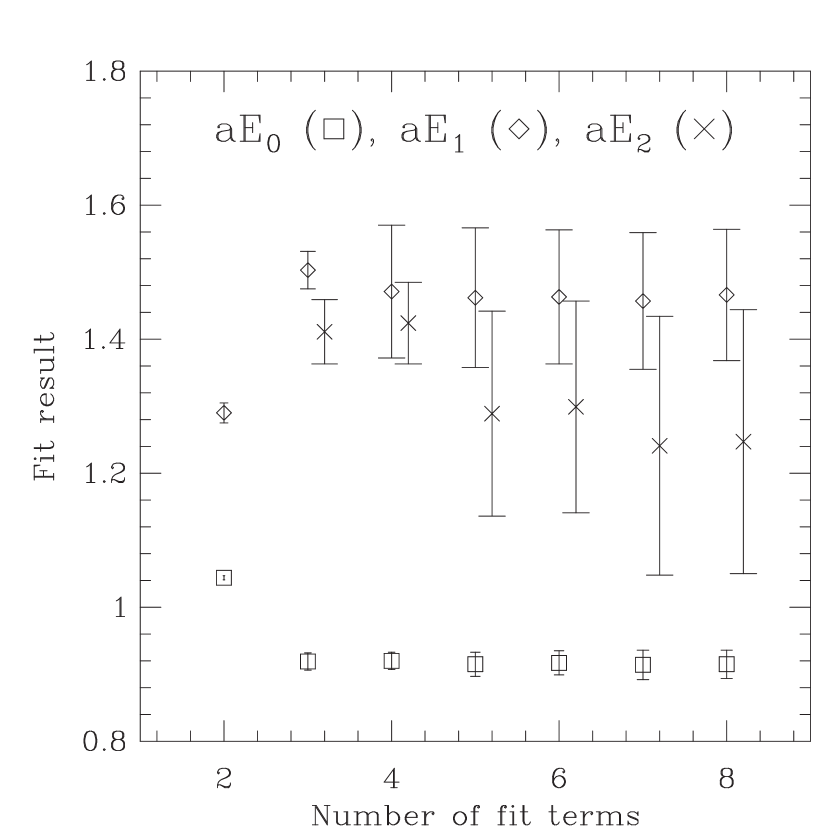
Figure 2: Results of several fits to Propagator of Fig. 1 plotted vs. number of exponentials in the fit. Parameters shown are the non-oscillating ground state energy ($aE_{0}$), the oscillating ground state energy ($aE_{1}$), and the non-oscillating first excited state energy ($aE_{2}=aE_{0}+a\Delta E_{2}$).

In Fig. 2 we plot the non-oscillating and oscillating ground state energies, as well as the first excited state energy, vs. the number $K$ of exponentials in the fit. The rest of the fit parameters are given in Tables 4 and 5. One can clearly see the stability of the ground state fit parameters $A_{0},E_{0}$ and $A_{1},E_{1}$ as $K$ is increased. The beginning of a plateau at $K=3$ implies at least one excited state is needed in the fit in order for the excited state effects to be removed from the ground states. Table 6 similarly indicates that $K\geq 3$ is necessary in order to have an “acceptable” $\chi^{2}_{\rm aug}/{\rm DoF}$; as we discuss in Appendix C, $\chi^{2}_{\rm aug}/{\rm DoF}$ should only be used as a gross check of the fit. E.g. $\chi^{2}_{\rm aug}/{\rm DoF}\gtrsim 2$ implies the fit function is a highly improbable model of the data, but one should not necessarily prefer a fit with $\chi^{2}_{\rm aug}/{\rm DoF}=0.8$ over one with $\chi^{2}_{\rm aug}/{\rm DoF}=1.3$.

Note that the uncertainties estimated from the fit for the ground state parameters are much smaller than the widths of the corresponding priors, while the errors from the fit are comparable to the prior widths for most of the excited state parameters. The first excited non-oscillating state, $k=2$, is an exception, appearing to be well constrained by the data until another non-oscillating state, $k=4$, is included in the fit. This means that the $K=3$ and $K=4$ fit result for $E_{2}$ does a good job of absorbing the effects of the excited states, but that there is not enough constraint from the data (or the priors) to separate the first excited state from the second. Thus, we conclude that $K=3$ is sufficient to obtain reliable estimates of the ground state energies and amplitudes and that the data is not sufficiently precise to extract excited state energies and amplitudes.

We are able to utilize this constrained curve fitting method to fit all of our data except in one case: the heavy-light correlators computed with the AsqTad action on the $8^{3}\times 20$ lattice. We were not able to find fits with $\chi^{2}_{\rm aug}/{\rm DoF}<8$; one example is shown in Fig. 3 where the fit is visibly much worse than for the 1-link action shown in Fig. 1. This turns out to be a consequence of using an action with next-to-next-to-nearest neighbor couplings in the $\hat{t}$-direction on a lattice with coarse temporal lattice spacing.

The free Naik fermion dispersion relation (see Fig. 4) has complex solutions which implies there may be excited states with negative norms contaminating the correlators at short time separations. If the temporal extent of the lattice were sufficiently long and sufficiently precise correlators were computed, these negative norm states which have energies proportional to $1/a$ would have a negligible effect: one could include only points with $t$ greater than some minimum value in the fit, or one could include a negative norm state in the fit. However, for the $8^{3}\times 20$ lattice where $1/a=0.8$ GeV we are unable to drop enough points and get a good fit while keeping enough to fit to states of both parities. Also, when we tried to include a negative norm exponential in the fit, large cancellations with the positive norm excited states resulted in unstable fit results.

We checked this hypothesis on the $1/a=0.8$ GeV lattice by simulating with 4 different staggered quark actions: the 1-link and improved actions as well as an action where the Naik term was included but no fattening of the links was done (the Naik action) and an action with fat-links but no Naik term (the “fat-link” action). We were able to obtain reasonable fits to heavy-light correlators with the 1-link and fat-link actions, but not with the Naik action nor the fully improved action; we tabulate typical values for $\chi^{2}_{\rm aug}/{\rm DoF}$ in Table 7. Furthermore we performed simulations on an anisotropic $8^{3}\times 48$ lattice with a very fine temporal lattice spacing $1/a_{t}=3.7$ GeV using the 1-link action, the AsqTad-tn action ($y_{t,{\rm naik}}=0$), and the full AsqTad action ($y_{t,{\rm naik}}=1$). In all 3 cases we found acceptable fits with similar values of $\chi^{2}_{\rm aug}/{\rm DoF}$, again tabulated in Table 7. Fig. 5 shows the pseudoscalar propagator on this lattice for the AsqTad action. We have no problem fitting to heavy-light correlators on a finer isotropic $12^{3}\times 32$ lattice where $1/a=1.0$ GeV with the $O\left(a^{2}\right)$ improved action. Therefore, the origin of the problematic fits on the $1/a=0.8$ GeV lattice is due to a particular lattice artifact arising from the temporal Naik term; but with a larger lattice scale $1/a\geq 1.0$ GeV these artifacts become insignificant.

Let us return to the subject of estimating the uncertainties of the fit parameters. The second derivative of $\chi^{2}_{\rm aug}$ (50) gives a reliable estimate of the uncertainty assuming that the priors are reasonable and that the data are approximately Gaussian. Resampling methods, such as the jackknife or the bootstrap, can be used to check whether the distributions are Gaussian, and they provide a simple check on statistical correlations between different fit parameters. Both procedures take many subsets of the data as estimates of the original set; performing a fit on each subset yields a distribution for each fit parameter from which an error estimate can be made. We employ the bootstrap method of resampling which requires some modification in order to properly handle the contributions of the priors: as we show in Appendix C one must randomly select new prior means $\mu_{\lambda_{i}}^{b}$ for each bootstrap fit Lepage et al. (2002). Table 8 shows the results of applying this bootstrap analysis to the heavy-light pseudoscalar correlator computed with the 1-link staggered action on the $8^{3}\times 20$ lattice. These results can be compared to those in Tables 4 and 5. We find both methods produce comparable error estimates. For ease of error propagation, we use bootstrap method to quote uncertainties in the results presented below.

IV Results

This section contains several results produced using the methods proposed and described above. The purpose of this study was to check the validity of this proposal, so the results presented below should not be construed as state-of-the-art calculations to be used for phenomenology. The results here show that NRQCD-staggered calculations produce results comparable to NRQCD-Wilson calculations – central values agree and statistical and fitting uncertainties are comparable – but at a fraction of the computational cost. A more complete calculation of the $B$ spectrum and decay constant on finer, unquenched configurations is underway which will exploit the advantages of improved staggered fermions to produce, we believe, the most accurate theoretical computation of those quantities to date.

IV.1 Light hadron masses and dispersion relations

As mentioned before we chose a value for the bare staggered mass $m$ so that the ratio of the light pseudoscalar mass to the light vector mass would be somewhat near the phenomenological value $\sqrt{2m_{K}^{2}-m_{\pi}^{2}}/m_{\phi}=0.673$. We use the pseudo Goldstone boson correlator ${\rm Tr}|G_{\chi}(x;0)|^{2}$ to compute the pseudoscalar meson mass and the correlator $(-1)^{x_{k}/a}\,{\rm Tr}|G_{\chi}(x;0)|^{2}$ to compute the vector meson mass. These masses and their ratio are listed in Table 9 for the different lattices and actions. Note that even on the $a^{-1}$= 0.8 GeV lattice the light hadron correlators from the AsqTad action do not suffer the contamination from the negative norm states which affected the heavy-light correlators, as discussed in Sec. III.2.

One measure of discretization effects is the dispersion relation. Specifically, we can compute the “speed-of-light” factor

$$c^{2}({\bf\bm{p}})~{}\equiv~{}\frac{E^{2}({\bf\bm{p}})-E^{2}(0)}{|{\bf\bm{p}}|^{2}}$$ (52)

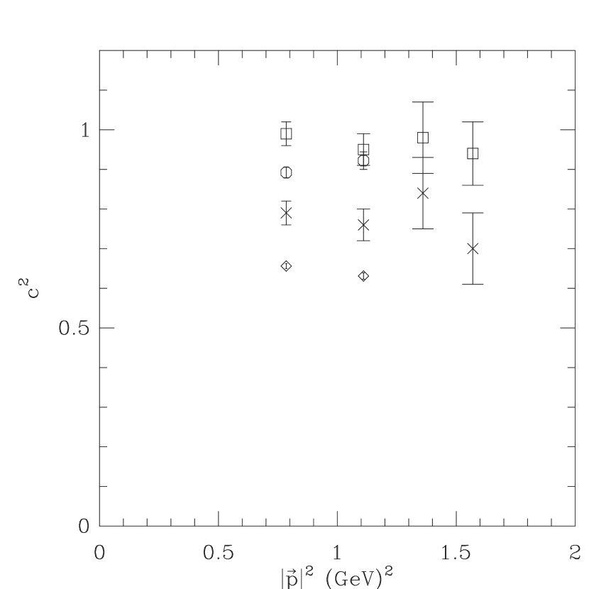
Figure 6: Pion speed-of-light squared vs. momenta on the coarse ($8^{3}\times 20$) lattice using several actions. The 1-link (diamonds) and AsqTad (circles) results are ours, compared to the clover (crosses) and D234 (squares) results of Alford et al. (1998).

which should equal 1 in the absence of lattice artifacts. The Naik term (38) is responsible for subtracting the $O\left(a^{2}\right)$ uncertainties in $c^{2}({\bf\bm{p}})$ and its success can be seen in the following results. Table 10 lists the values of $c^{2}$ computed with several values of momentum (averaged over all equivalent orientations in momentum space). On the coarser lattice ($\beta=1.719$) one can see that using fat links does not improve $c^{2}$ much compared to the 1-link action, but adding only the Naik term to the 1-link action results in a significant improvement. This is borne out on the finer lattice ($\beta=2.131$), where the AsqTad action has an improved $c^{2}$. Fig. 6 shows comparison of $c^{2}({\bf\bm{p}})$ between these results and those for improved Wilson actions Alford et al. (1998). The AsqTad action has a better pion dispersion relation than the clover action, but not quite as good as the D234 action.

On the anisotropic lattices we use this quantity to tune the bare parameter $c_{0}$ in (39); it is adjusted so that the pion speed-of-light parameter $c^{2}({\bf\bm{p}})\approx 1$. Table 11 lists the values of $c_{0}$ we used and the resulting computed values of $c^{2}$ for several momenta.

IV.2 Finite momentum $B_{s}$ and its mass

The energies, $E_{\rm sim}({\bf\bm{p}})$, extracted from correlation functions include an unknown but momentum independent shift due to the neglect of the heavy quark rest mass, i.e.

$$E_{\rm sim}({\bf\bm{p}})=E({\bf\bm{p}})-\Delta$$ (53)

where $E({\bf\bm{p}})$ is the physical energy. In perturbation theory, the shift $\Delta$ is the difference between the renormalized pole mass and the constant part of the heavy quark self-energy:

$$\Delta_{\rm pert}~{}=~{}Z_{m}M_{0}-E_{0}\,.$$ (54)

Given $E_{\rm sim}(0)$ from a simulation, the physical mass of a hadron can be computed through

$$M_{\rm pert}~{}\equiv~{}E_{\rm sim}(0)+Z_{M}M_{0}-E_{0}$$ (55)

where we attach the label “pert” to denote that the perturbative shift $\Delta_{\rm pert}$ was used. For the finer isotropic lattice and the $1/M$ NRQCD action with $aM_{0}=5.0$ we find

$$Z_{M}M_{0}-E_{0}~{}=~{}M_{0}-0.890\,\alpha_{s}+M_{0}\,O\left(\alpha_{s}^{2}\right)$$ (56)

The results obtained on the finer isotropic lattice, using the AsqTad staggered action, give $M_{\rm pert}(B_{s})=5.55\pm 0.45$ GeV and $M_{\rm pert}(B_{s}^{*})=5.58\pm 0.45$ GeV. The numerical size of the $O\left(\alpha_{s}^{2}\right)$ uncertainty is estimated by taking $\alpha_{s}\approx 0.3$, a typical value for quenched lattices with these spacings, and assuming the coefficient of the $O\left(\alpha_{s}^{2}\right)$ term is 1 (times $M_{0}$ as indicated in (56)).

The physical mass can also be calculated nonperturbatively, using the dispersion relation

$$E^{2}({\bf\bm{p}})=M^{2}+|{\bf\bm{p}}|^{2}\,.$$ (57)

In order to cancel the unknown shift in (53), we consider $(E({\bf\bm{p}})-E(0))^{2}=(E_{\rm sim}({\bf\bm{p}})-E_{\rm sim}(0))^{2}$, which we square and solve for the mass

$$M_{\rm kin}~{}\equiv~{}\frac{|{\bf\bm{p}}|^{2}-[E_{\rm sim}({\bf\bm{p}})-E_{\rm sim}(0)]^{2}}{2[E_{\rm sim}({\bf\bm{p}})-E_{\rm sim}(0)]}\,.$$ (58)

When the mass is computed using (58), we call it the kinetic mass, to distinguish it from the perturbative result $M_{\rm pert}$. Setting $|{\bf\bm{p}}|=2\pi/12a=0.52$ GeV, the kinetic masses on the finer isotropic lattice (with the AsqTad light quark action) are $M_{\rm kin}(B_{s})=5.56\pm 0.33$ GeV and $M_{\rm kin}(B_{s}^{*})=5.68\pm 0.33$ GeV.

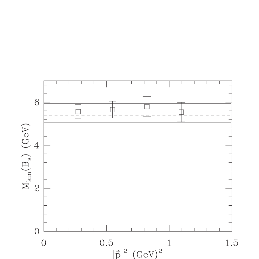
Figure 7: Kinetic mass for the $B_{s}$ meson on the $12^{3}\times 32$ lattice with the improved staggered action ($am=0.10$) and the $1/M$ NRQCD action ($aM_{0}=5.0$). Computed using (58). The dashed line marks the experimental measurement $M_{B_{s}}=5.37$ GeV, and the solid lines show the range given perturbatively.

Figs. 7 and 8 show the kinetic masses for the $B_{s}$ and $B_{s}^{*}$ for several momenta. We find excellent agreement between the perturbative and nonperturbative calculations of the mass. Furthermore, the consistency of the kinetic masses over several momenta demonstrate that the combined NRQCD–improved staggered formulation gives the correct dispersion relation for $B_{s}$ and $B_{s}^{*}$ up to $|{\bf\bm{p}}|=\pi/3a=1.1$ GeV. One should not put too much weight on any agreement or disagreement between the calculation and experiment, given that the calculation is quenched, the lattice spacing not precisely determined, and the quark masses not precisely tuned.

IV.3 Mass splittings in the $B_{s}$ system

Since the shift $\Delta$ between simulation energy and the physical energy (Eq. 53) is entirely due to the NRQCD action, it is universal for all bound states with the heavy quark. Therefore, we can compute mass splittings much more precisely than suggested by the uncertainties in $M_{\rm kin}$ and $M_{\rm pert}$. The splittings we compute on various lattices which correspond to the $B_{s}$ system are given in Table 14; below are a few remarks concerning the different calculations.

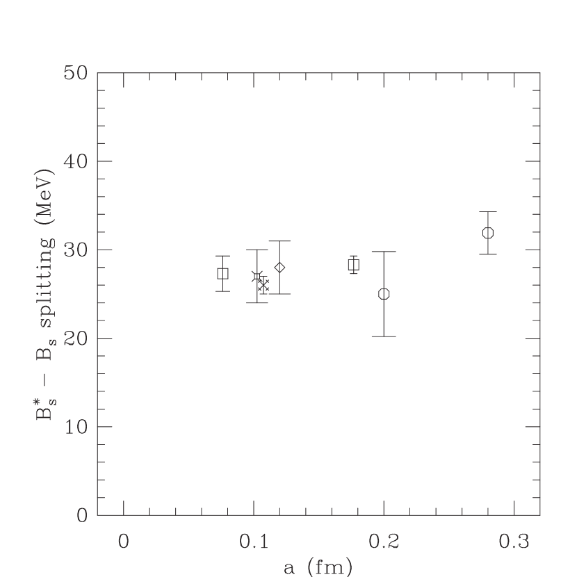
Figure 9: The hyperfine splitting between $B_{s}$ and $B_{s}^{*}$ computed on quenched lattices. Our NRQCD-staggered results (from the isotropic lattices) are the circles. The squares come from Hein et al. (2000), the fancy square from Ali Khan et al. (2000), and the diamond from Ishikawa et al. (2000) which all used an NRQCD-clover action, and the fancy cross comes from an NRQCD-D234 calculation Lewis and Woloshyn (2000). All tune the heavy quark mass as in this work (see text for elaboration). For comparison, the experimental measurement is $47.0\pm 2.6$ MeV Hagiwara et al. (2002). Error bars are statistical only.

The hyperfine splitting $M_{B_{s}^{*}}-M_{B_{s}}$ is the most straightforward to compute since it is the difference between the $E_{\rm sim}$ for the non-oscillating ground states of the vector and pseudoscalar correlators. The results are comparable to previous quenched lattice studies; Figure 9 shows our quenched results on the 2 isotropic lattices compared to results published in Refs. Ali Khan et al. (2000); Ishikawa et al. (2000); Hein et al. (2000); Lewis and Woloshyn (2000). This splitting was also computed using NRQCD in Ref. Lewis and Woloshyn (1998), but they have different systematic errors caused by the quenched approximation, specifically they set the bare bottom quark mass by tuning the $\Upsilon$ mass, instead of a heavy-light mass. Our error bars are larger than those for most other results for two reasons. The first is simply that this work is based on 200 configurations compared to 300 Ishikawa et al. (2000), 278 and 212 Hein et al. (2000), and 2000 Lewis and Woloshyn (2000) (Ref. Ali Khan et al. (2000) used 102 configurations). The second is that the Bayesian curve fitting method includes as part of the quoted uncertainty an estimation of the error due to excited state contamination, in contrast to the single exponential fits used in previous work.

Quenched results have an inherent ambiguity depending on which physical quantities are used to set the lattice spacing and bare quark masses. Preliminary results on unquenched lattices indicate that the inclusion of sea quarks yields a unique scale and bottom quark masses Gray et al. (2002) and give a $B_{s}^{*}-B_{s}$ splitting Wingate et al. (2002) consistent with the experimental measurement $M_{B_{s}^{*}}-M_{B_{s}}=47.0\pm 2.6$ MeV Hagiwara et al. (2002).

The $L=1$, or “P-wave”, states $B_{s0}^{*}$ and $B_{s1}$ have the same quantum numbers as the oscillating states in the pseudoscalar and vector correlators, respectively. The fact that $E_{\rm sim}$ for these states can be computed using the same correlator data as the $L=0$ states should be another advantage over formulations with Wilson-like quarks. In practice, however, it appears that the coupling of these states to the local-local correlator is rather small and consequently the fitting uncertainties for these splittings are large. Smeared sources and sinks for both heavy and light quark propagators should be explored as methods for amplifying the coupling to the $P$-wave states. In Table 14 we list some combinations of splittings.

IV.4 Decay constant

The heavy-light decay constants are defined through the matrix element of the electroweak axial vector current

$$\langle 0|A_{0}|B_{s}\rangle~{}=~{}\langle 0|\;\overline{q}\,\gamma_{5}\gamma_{0}\,b\;|B_{s}\rangle~{}=~{}f_{B_{s}}M_{B_{s}}\,.$$ (59)

The fields in the current above are those defined in the Standard Model, so a matching must be performed between them and the fields of our lattice action. The continuum heavy quark field $b$ is related to the nonrelativistic field $\phi$ through the Foldy-Wouthuysen-Tani transformation

$$b~{}=~{}\left(1-\frac{\bm{\gamma\cdot\nabla}}{2M_{0}}~{}+~{}O\left(\left(\frac{\Lambda_{\rm QCD}}{M}\right)^{2}\right)\right)Q$$ (60)

where

$$Q~{}=~{}\left(\begin{array}[]{c}\phi\\ 0\end{array}\right)\,.$$ (61)

Expanding the QCD axial-vector current in terms of NRQCD operators up to $O\left(\Lambda_{\rm QCD}/M\right)$ and at $O\left(\alpha_{s}\right)$ in perturbation theory yields a combination of the three operators

$$J_{0}^{(0)} = \overline{\Psi}\,\gamma_{5}\gamma_{0}\,Q$$ (62)

$$J_{0}^{(1)} = -\frac{1}{2M_{0}}\overline{\Psi}\,\gamma_{5}\gamma_{0}\,{\bf\bm{\gamma\cdot\nabla}}\,Q$$ (63)

$$J_{0}^{(2)} = \frac{1}{2M_{0}}\overline{\Psi}\,\bm{\gamma\cdot\stackrel{{\scriptstyle\leftarrow}}{{\nabla}}}\,\gamma_{5}\gamma_{0}\,Q\,.$$ (64)

The operator equation is then written as

$$A_{0}~{}\doteq~{}(1+\alpha_{s}\rho_{0})J_{0}^{(0)}+(1+\alpha_{s}\rho_{1})J_{0}^{(1)}+\alpha_{s}\rho_{2}J_{0}^{(2)}\,.$$ (65)

The symbol $\doteq$ is meant to imply that matrix elements of the operators on the left and right hand sides are equal, up to whatever order in the effective theory we are working. Since we are neglecting terms of order $\alpha_{s}\Lambda_{\rm QCD}/M$ the terms proportional to $\rho_{1}$ and $\rho_{2}$ are dropped from our analysis. The relation we use to do the matching is

$$A_{0}~{}\doteq~{}(1+\alpha_{s}\widetilde{\rho}_{0})J_{0}^{(0)}\;+\;J_{0}^{(1,{\rm sub})}$$ (66)

where the $1/(aM)$ power law mixing of $J_{0}^{(1)}$ with $J_{0}^{(0)}$ is absorbed at one-loop level into a subtracted $\Lambda_{\rm QCD}/M$ current Collins et al. (2001b)

$$J_{0}^{(1,{\rm sub})}~{}\equiv~{}J_{0}^{(1)}-\alpha_{s}\zeta_{10}J_{0}^{(0)}\,,$$ (67)

and $\widetilde{\rho}_{0}-\zeta_{10}=\rho_{0}$.

Since the heavy spinor obeys $\gamma_{5}\gamma_{0}Q=\gamma_{5}Q$, the matrix element ${\langle 0|J_{0}^{(0)}|B_{s}\rangle}$ is related simply to the ground state amplitude of the pseudoscalar heavy-light correlator $C_{B}^{(2)}({\bf\bm{p}}=0,t)$. Let us denote this amplitude by $C_{00}$, then

$$C_{00}~{}=~{}\frac{|\langle 0|J_{0}^{(0)}|B_{s}\rangle|^{2}}{2M_{B_{s}}}\,.$$ (68)

To get the $\Lambda_{\rm QCD}/M$ current matrix element we compute correlators where we put $J_{0}^{(1)}$ at the sink. Let us denote the ground state amplitude of this correlator by $C_{10}$, then

$$C_{10}~{}=~{}\frac{\langle 0|J_{0}^{(1)}|B_{s}\rangle\langle B_{s}|J_{0}^{(0),\dagger}|0\rangle}{2M_{B_{s}}}\,.$$ (69)

As mentioned before, we concentrate on the quenched $12^{3}\times 32$ lattice which is closest to the target unquenched configurations, albeit coarser. Fits to these correlators, shown in Fig. 10, yield the bootstrapped ratio

$$\frac{\langle 0|J_{0}^{(1)}|B_{s}\rangle}{\langle 0|J_{0}^{(0)}|B_{s}\rangle}~{}=~{}-0.064\pm 0.005~{}{\rm(stat).}$$ (70)

The $1/M$ NRQCD action is used for this calculation, for which we compute (with $aM_{0}=5.0$) $\widetilde{\rho}_{0}=0.208\pm 0.003$ and $\zeta_{10}=-0.0997$. Performing the subtraction (67) we find

$$\frac{\langle 0|J_{0}^{(1,{\rm sub})}|B_{s}\rangle}{\langle 0|J_{0}^{(0)}|B_{s}\rangle}~{}=~{}-0.034\pm 0.004~{}{\rm(stat).}$$ (71)

This ratio can be compared to other lattice formulations; it is the “physical” $\Lambda_{\rm QCD}/M$ correction to $J_{0}^{(0)}$ with $1/a$ power law effect subtracted at the one-loop level. The 3.4(4)% correction we find on the $a^{-1}$ $=1.0$ GeV lattice is in excellent agreement with the 3-5% corrections found using the NRQCD and clover actions on lattices with inverse spacings from 1.1 – 2.6 GeV Collins et al. (2001b). Note that even on the finest lattice in Ref. Collins et al. (2001b), where power law contributions are the largest, the one-loop subtraction takes ${\langle 0|J_{0}^{(1)}|B_{s}\rangle}/{\langle 0|J_{0}^{(0)}|B_{s}\rangle}=-14\%$ to ${\langle 0|J_{0}^{(1,{\rm sub})}|B_{s}\rangle}/{\langle 0|J_{0}^{(0)}|B_{s}\rangle}=-4\%$, in agreement with calculations on coarser lattices. Given the present agreement between our result and that of Ref. Collins et al. (2001b), we can expect a similarly successful subtraction in our ongoing calculation with the unquenched MILC ensemble.

Applying (66) and (59) gives the quenched result

$$f_{B_{s}}~{}=~{}225\pm 9{\rm(stat)}\pm 20{\rm(p.t.)}\pm 27{\rm(disc.)}~{}{\rm MeV.}$$ (72)

The 20 MeV perturbative uncertainty is the estimate of the $O\left(\alpha_{s}^{2}\right)$ error in (66), obtained by taking $\alpha_{s}\approx 0.3$ and a coefficient equal to 1. The other perturbative uncertainties, due to one-loop corrections to the coefficients in the action and in the operator matching, are $O\left(\alpha_{s}\Lambda_{\mathrm{QCD}}/M\right)$ which is estimated to be 2.4%, assuming $\Lambda_{\mathrm{QCD}}$ = 400 MeV (and using $M_{0}=5.0$ GeV). The 27 MeV discretization error is our estimate of the $O\left(\alpha_{s}a\Lambda_{\rm QCD}\right)$ error in the current $J_{0}^{(0)}$ (62); again we assume the leading correction term comes with a coefficient of order 1. This error may be reduced to $O\left(\alpha_{s}(a\Lambda_{\rm QCD})^{2}\right)$ by improving $J_{0}^{(0)}$ à la Symanzik, which requires calculation of $\rho_{1}$ and $\rho_{2}$ in (65) Shigemitsu (1998); Morningstar and Shigemitsu (1998). Finally, note that we have included the $O\left(\alpha_{s}/aM\right)$ power-law correction; we would have estimated this to be a 6% effect, but it was calculated to be 3% (compare 70 and 71). Given those uncertainties, we find agreement with the recent quenched world average $f_{B_{s}}~{}=~{}200\pm 20$ MeV Ryan (2002).

V Conclusions

We believe the methods outlined within this paper provide the quickest route to accurate calculations of $B$ meson masses and decay constants on realistic unquenched lattices. Improved staggered fermions have several advantages over Wilson-like fermions and are far less expensive to simulate than domain wall or overlap fermions. The equivalence between naive and staggered fermions greatly simplifies the construction of operators which couple to states of interest. The fact that the NRQCD action does not have a doubling symmetry leads to taste-changing suppression in heavy-light mesons, avoiding the ambiguities of the light staggered hadrons.

We have presented results on several types of lattices, the most important being the finer of the two isotropic lattices since it is most similar to the unquenched MILC lattices. The results from these simulations have no unpleasant surprises: they agree with results produced by previous quenched simulations. Therefore, we can trust this formulation when it is used in parts of parameter space inaccessible to other formulations.

Appendix A Formalism details

In this Appendix we present a more detailed analysis of the heavy-light operators used in the numerical calculation.

Since naive fermions have 16 taste degrees-of-freedom, there is the possibility of forming 16 different $B$ mesons labeled by the light taste index $g$, i.e. $B_{g}$. The general choice for a $B_{g}$ meson interpolating heavy-light operator takes on the form

$${\cal W}_{B_{g}}(x)=\overline{\Psi}_{H}(x)\gamma_{5}M_{g}e^{i\pi_{g}\cdot x}\Psi(x)$$ (73)

The 16 different operators lead to degenerate states, since they are related by the symmetry transformation (II.1). It is sufficient to work with just one of the 16 choices to extract all the relevant physics. In our simulations we usually use the simplest choice $g=\emptyset$, i.e. Eq. (25). Any other choice would have served equally well. For instance, consider the case $g=\mu_{j}$ with $\mu_{j}$ equal to one of the spatial directions and carry out a sum over spatial sites. Eq. (73) then becomes

$$a^{3}\,\sum_{{\bf\bm{x}}}{\cal W}_{B_{j}}(x)=a^{3}\,\sum_{{\bf\bm{x}}}\overline{\Psi}_{H}(x)\gamma_{5}M_{j}e^{i\pi_{j}\cdot x}\Psi(x)=a^{3}\,\sum_{{\bf\bm{x}}}\overline{\Psi}_{H}(x)i\gamma_{j}e^{i\pi_{j}\cdot x}\Psi(x).$$ (74)

One sees that the zero spatial momentum $B_{j}$ meson operator is identical to an operator one would superficially (and incorrectly) associate with a $B^{*}$ meson of polarization “$j$” with momentum $\pi/a$ in the $j^{th}$ direction. The correct interpretation of (74) is that it represents a zero momentum pseudoscalar heavy-light meson. This will become more evident when we look at the operator ${\cal W}_{B_{g}}(x)$ in momentum space. We have verified that the RHS of (74) gives identical correlators, configuration-by-configuration, to (25) (the latter summed over space). (In fact, the symmetries of (II.1) provide excellent tests of one’s simulation codes.) Therefore, it is sufficient to work with just one type of $B$ meson operator, e.g. with just (25).

In order to delve further into the Lorentz quantum number and taste content of the interpolating operators ${\cal W}_{B_{g}}(x)$ we will look at this operator in momentum space. In terms of the “tilde” fields (26) one has (we take the case where $g$ does not include a temporal component; the latter case can be discussed in a completely analogous way)

$$a^{3}\,\sum_{{\bf\bm{x}}}{\cal W}_{B_{g}}({\bf\bm{x}},t) = \int_{{\bf\bm{k}},D_{s}}\overline{\tilde{\psi}_{H}}({\bf\bm{k}},t)\,\gamma_{5}M_{g}\,\tilde{\psi}({\bf\bm{k}}+{\bf\bm{\pi}}_{g},t)$$ (75)

$$= \sum_{g_{s}\in G_{s}}\int_{{\bf\bm{k}},D_{s,\emptyset}}\overline{\tilde{\psi}_{H}}({\bf\bm{k}}+{\bf\bm{\pi}}_{g_{s}},t)\,\gamma_{5}M_{g}\,\tilde{\psi}({\bf\bm{k}}+{\bf\bm{\pi}}_{g}+{\bf\bm{\pi}}_{g_{s}},t)$$

We extract the taste content of this bilinear by writing

$$\tilde{\psi}({\bf\bm{k}}+{\bf\bm{\pi}}_{g}+{\bf\bm{\pi}}_{g_{s}},t) = \int^{\pi/a}_{-\pi/a}\frac{dk_{0}}{2\pi}e^{ik_{0}t}\psi({\bf\bm{k}}+{\bf\bm{\pi}}_{g}+{\bf\bm{\pi}}_{g_{s}},k_{0})$$ (76)

$$= \int^{\pi/2a}_{-\pi/2a}\frac{dk_{0}}{2\pi}e^{ik_{0}t}\left[\psi({\bf\bm{k}}+{\bf\bm{\pi}}_{g}+{\bf\bm{\pi}}_{g_{s}},k_{0})+(-1)^{t}\psi({\bf\bm{k}}+{\bf\bm{\pi}}_{g}+{\bf\bm{\pi}}_{g_{s}},k_{0}+\pi_{g_{t}})\right]$$

$$= \int^{\pi/2a}_{-\pi/2a}\frac{dk_{0}}{2\pi}e^{ik_{0}t}\left[M_{g_{s}g}^{\dagger}q^{g_{s}g}({\bf\bm{k}},k_{0})+(-1)^{t}M^{\dagger}_{g_{t}g_{s}g}q^{g_{t}g_{s}g}({\bf\bm{k}},k_{0})\right]$$

so that

$$a^{3}\,\sum_{{\bf\bm{x}}}{\cal W}_{B_{g}}({\bf\bm{x}},t) = \sum_{g_{s}\in G_{s}}\int_{{\bf\bm{k}},D_{s,\emptyset}}\int^{\pi/2a}_{-\pi/2a}\frac{dk_{0}}{2\pi}e^{ik_{0}t}$$ (77)

$$\left\{\overline{\tilde{\psi}}_{H}({\bf\bm{k}}+{\bf\bm{\pi}}_{g_{s}},t)\,\gamma_{5}M_{g}\left[M_{g_{s}g}^{\dagger}q^{g_{s}g}({\bf\bm{k}},k_{0})+(-1)^{t}M^{\dagger}_{g_{t}g_{s}g}q^{g_{t}g_{s}g}({\bf\bm{k}},k_{0})\right]\right\}$$

Since there is no doubling symmetry for the heavy quark action, the field $\overline{\tilde{\psi}}_{H}({\bf\bm{k}}+{\bf\bm{\pi}}_{g_{s}},t)$, for ${\bf\bm{\pi}}_{g_{s}}\neq{\bf\bm{\pi}}_{\emptyset}$, represents a heavy quark with large spatial momentum. Consequently, even though the operator in (77) couples to zero momentum meson states, the states corresponding to $g\neq\emptyset$ are very energetic. This is precisely the important difference between studying heavy-light and light-light mesons with light staggered quarks.

We will estimate the effect of the $g_{s}\neq\emptyset$ sectors below, however the lowest energy state, and consequently the dominant contributions to a ${\cal W}_{B_{g}}({\bf\bm{x}},t)$ correlator, will come from the region $g_{s}=\emptyset$ in the sum $\sum_{g_{s}}$.

$$a^{3}\,\sum_{{\bf\bm{x}}}{\cal W}_{B_{g}}({\bf\bm{x}},t) \rightarrow \int_{{\bf\bm{k}},D_{s,\emptyset}}\int^{\pi/2a}_{-\pi/2a}\frac{dk_{0}}{2\pi}e^{ik_{0}t}$$ (78)

$$\left\{\overline{\tilde{\psi}}_{H}({\bf\bm{k}},t)\,\gamma_{5}\,\left[q^{g}({\bf\bm{k}},k_{0})+(-1)^{t}M^{\dagger}_{g_{t}}q^{g_{t}g}({\bf\bm{k}},k_{0})\right]\right\}$$

The non-oscillating contribution is the $B_{g}$ meson of taste $g$. Its parity partner is a $0^{+}$ meson, usually called the $J=0$ $P-$state. It is remarkable that both $S-$ and $P-$states can be obtained from a single correlator. Note also that the combination $\overline{\tilde{\psi}}_{H}({\bf\bm{k}},t)\,\gamma_{5}\,q^{g}({\bf\bm{k}},k_{0})$, with its obviously pseudoscalar Lorentz structure holds for all tastes $g$, i.e. for trivial and nontrivial $M_{g}$ in (73).

We discuss next those terms omitted upon going from (77) to (78). Take for instance the contribution from $g_{s}\rightarrow gl\equiv\mu_{l}$ with “$l$” equal to one of the spatial directions. The non-oscillatory term becomes

$$\overline{\tilde{\psi}}_{H}({\bf\bm{k}}+{\bf\bm{\pi}}_{gl},t)\,\gamma_{5}M_{gl}\,q^{gl\,g}({\bf\bm{k}},k_{0})=\overline{\tilde{\psi}}_{H}({\bf\bm{k}}+{\bf\bm{\pi}}_{gl},t)\,i\gamma_{l}\,q^{gl\,g}({\bf\bm{k}},k_{0}).$$ (79)

One sees that the Lorentz structure is that of a $1^{-}$ particle. However, since the heavy quark has very high momentum and no doublers, this intermediate state is highly virtual. Such states would appear in fits to correlation functions as extra structure at energies of order $\Delta E\approx 1/(Ma^{2})$. These lattice artifacts can also affect low energy states through loops; their effects can be estimated perturbatively and are part of the $O\left(\alpha_{s}a^{2}\right)$ errors inherent in the action. Such errors can be removed, if need be, by perturbatively improving the action further, but there is little evidence that they are important at practical values of the lattice spacing.

Appendix B Discrete derivatives and field strengths

Here we write explicitly the higher order tadpole-improved derivatives and improved field strength tensor used in the fermion actions.

$$\nabla^{(2)}_{\mu}\,\Psi(x) = \frac{1}{u_{\mu}}\,[U_{\mu}(x)\Psi(x+a_{\mu})\;+\;U^{\dagger}_{\mu}(x-a_{\mu})\Psi(x-a_{\mu})]$$ (80)

$$\;-\;2\,\Psi(x)$$

$$\nabla^{(3)}_{\mu}\,\Psi(x) = \frac{1}{2}\,\frac{1}{u^{2}_{\mu}}\,[U_{\mu}(x)U_{\mu}(x+a_{\mu})\Psi(x+2a_{\mu})$$ (81)

$$\;-\;U^{\dagger}_{\mu}(x-a_{\mu})U^{\dagger}_{\mu}(x-2a_{\mu})\Psi(x-2a_{\mu})]$$

$$-\,\frac{1}{u_{\mu}}\,[U_{\mu}(x)\Psi(x+a_{\mu})\;-\;U^{\dagger}_{\mu}(x-a_{\mu})\,\Psi(x-a_{\mu})]$$

$$\nabla^{(4)}_{\mu}\,\Psi(x) = \frac{1}{u^{2}_{\mu}}\,[U_{\mu}(x)U_{\mu}(x+a_{\mu})\Psi(x+2a_{\mu})$$ (82)

$$\;+\;U^{\dagger}_{\mu}(x-a_{\mu})U^{\dagger}_{\mu}(x-2a_{\mu})\Psi(x-2a_{\mu})]$$

$$-\,4\,\frac{1}{u_{\mu}}\,[U_{\mu}(x)\Psi(x+a_{\mu})\;+\;U^{\dagger}_{\mu}(x-a_{\mu})\,\Psi(x-a_{\mu})]$$

$$\;+\;6\,\Psi(x)$$

The covariant derivatives acting on link matrices are defined as follows:

$$\frac{1}{u_{\nu}}\nabla_{\mu}\,U_{\nu}(x) = \frac{1}{u_{\mu}^{2}u_{\nu}}\,\Big{[}U_{\mu}(x)\,U_{\nu}(x+a_{\mu})\,U^{\dagger}_{\mu}(x+a_{\nu})$$ (83)

$$\;-\;U^{\dagger}_{\mu}(x-a_{\mu})\,U_{\nu}(x-a_{\mu})\,U_{\mu}(x-a_{\mu}+a_{\nu})\Big{]}$$

$$\frac{1}{u_{\nu}}\nabla^{(2)}_{\mu}\,U_{\nu}(x) = \frac{1}{u_{\mu}^{2}u_{\nu}}\,\Big{[}U_{\mu}(x)\,U_{\nu}(x+a_{\mu})\,U^{\dagger}_{\mu}(x+a_{\nu})$$ (84)

$$\;+\;U^{\dagger}_{\mu}(x-a_{\mu})\,U_{\nu}(x-a_{\mu})\,U_{\mu}(x-a_{\mu}+a_{\nu})\Big{]}$$

$$-\frac{2}{u_{\nu}}\,U_{\nu}(x)$$

The field strength operator $F_{\mu\nu}(x)$ is constructed from the so-called clover operator $\Omega_{\mu\nu}(x)$

$$F_{\mu\nu}(x) = {1\over 2i}\left(\Omega_{\mu\nu}(x)-\Omega^{\dagger}_{\mu\nu}(x)\right),$$

$$\Omega_{\mu\nu}(x) = \!{1\over 4u_{\mu}^{2}u_{\nu}^{2}}\!\sum_{{\{(\alpha,\beta)\}}_{\mu\nu}}\!\!\!\!U_{\alpha}(x)U_{\beta}(x\!+\!a_{\alpha})U_{-\alpha}(x\!+\!a_{\alpha}\!+\!a_{\beta})U_{-\beta}(x\!+\!a_{\beta})$$ (85)

where the sum is over $\{(\alpha,\beta)\}_{\mu\nu}=\{(\mu,\nu),(\nu,-\mu),(-\mu,-\nu),(-\nu,\mu)\}$ for $\mu\neq\nu$ and $U_{-\mu}(x+a_{\mu})\equiv U^{\dagger}_{\mu}(x)$. The $O\left(a^{2}\right)$ improved field strength tensor is

$$\tilde{F}_{\mu\nu}(x)~{}=~{}\frac{5}{3}F_{\mu\nu}(x) - \frac{1}{6}\Bigg{[}\,\frac{1}{u_{\mu}^{2}}(\,U_{\mu}(x)F_{\mu\nu}(x+a_{\mu})U^{\dagger}_{\mu}(x)$$ (86)

$$+ U^{\dagger}_{\mu}(x-a_{\mu})F_{\mu\nu}(x-a_{\mu})U_{\mu}(x-a_{\mu})\,)-(\mu\leftrightarrow\nu)\,\Bigg{]}$$

$$+ \frac{1}{6}\,(\frac{1}{u_{\mu}^{2}}+\frac{1}{u_{\nu}^{2}}-2)\,F_{\mu\nu}(x).$$

Appendix C Fitting details

In this Appendix we give a pedagogical discussion of the constrained curve fitting proposed in Lepage et al. (2002).

Recall that the standard fitting procedure is to minimize the $\chi^{2}$ function, or equivalently, to maximize the likelihood of the data, $C(t)$, given a set of fit parameters. The likelihood probability is given, up to a normalization constant, by

$$\mathcal{P}(C(t)|f(t;{\bm{\lambda}}),I)~{}\propto~{}\exp\left(-\frac{\chi^{2}}{2}\right)$$ (87)

where $I$ represents any unstated assumptions. Explicitly,

$$\chi^{2}~{}=~{}\sum_{t,t^{\prime}}\Big{(}\langle C(t)\rangle-f(t;{\bm{\lambda}})\Big{)}\,K_{t,t^{\prime}}^{-1}\,\Big{(}\langle C(t^{\prime})\rangle-f(t^{\prime};{\bm{\lambda}})\Big{)}\,.$$ (88)

The correlation matrix, $K$, is constructed to take into account correlations between $C(t)$ and $C(t^{\prime})$:

$$K_{t,t^{\prime}}~{}\equiv~{}\frac{1}{N-1}\;\left\langle\Big{(}C(t)-\langle C(t)\rangle\Big{)}\Big{(}C(t^{\prime})-\langle C(t^{\prime})\rangle\Big{)}\right\rangle\,.$$ (89)

with $N$ equal to the number of measurements.

Usually one cannot include enough terms in the fit to account for excited state contributions before the algorithm for minimizing $\chi^{2}$ breaks down. The minimization algorithm diverges as it searches in directions of parameter space which are unconstrained by the data. In the past the solution has been to limit the number of fit terms, then discard data by including $C(t)$ for $t\geq t_{\rm min}>0$; the optimal value of $t_{\rm min}$ is selected by a combination of looking for $\chi^{2}/{\rm DoF}=1$, maximizing the confidence level (Q factor), and observing plateaux in effective masses. A major weakness of this procedure is that it provides no estimate of the error due to omitting the excited states from the fit.

The constrained curve fitting method of Lepage et al. (2002), by using Bayesian ideas, allows one to incorporate the uncertainties due to poorly constrained states by relaxing the assumption that there are only a few states which saturate the correlation function. Bayesian fits maximize the probability that the fit function describes the given data, written as $\mathcal{P}(f(t;{\bm{\lambda}})|C(t),I)$; this probability is related to the likelihood (87) by Bayes’ theorem

$$\mathcal{P}(f(t;{\bm{\lambda}})|C(t),I)~{}=~{}\mathcal{P}(f(t;{\bm{\lambda}})|I)\;\frac{\mathcal{P}(C(t)|f(t;{\bm{\lambda}}),I)}{\mathcal{P}(C(t)|I)}$$ (90)

and is called the posterior probability. The denominator in (90) is treated as a normalization and plays no role in finding an optimal set of fit parameters. On the other hand, the prefactor, $\mathcal{P}(f(t;{\bm{\lambda}})|I)$, which multiplies the likelihood is the prior probability; its inclusion is what permits fits to many parameters.

The prior probability contains whatever assumptions about the values of the fit parameters one can safely make without looking at the data. In our case of fitting meson correlators, before any fitting is done one has an idea of a range of possible values for the amplitudes $A_{k}$ and energies $E_{k}$. Given such a range, the least informative prior distribution is a Gaussian with mean $\mu$ and half-width $\delta$, in which case the prior probability is given by

$$\mathcal{P}(f(t;{\bf\bm{\lambda}})|I)~{}=~{}\prod_{i=0}^{2K-1}\frac{1}{\delta_{\lambda_{i}}\sqrt{2\pi}}\;\exp\left(\frac{(\lambda_{i}-\mu_{\lambda_{i}})^{2}}{2\delta_{\lambda_{i}}^{2}}\right)$$ (91)

We sometimes refer to the set of $\{\mu_{i},\delta_{i}\}$ as the “priors.” The quantity which is minimized in the fits is

$$\chi^{2}_{\rm aug}(C(t),\{\lambda_{i}\},\{(\mu_{i},\delta_{i})\}) \equiv \chi^{2}(C(t),\{\lambda_{i}\})~{}+~{}\sum_{i=0}^{2K-1}\frac{(\lambda_{i}-\mu_{\lambda_{i}})^{2}}{\delta_{\lambda_{i}}^{2}}$$

$$\propto -2\ln\mathcal{P}(f(t;{\bm{\lambda}})|C(t),I)\;.$$

Expression (C) highlights how the prior distribution stabilizes the minimization algorithm. As one increases the number of fit parameters the terms from the prior in (C) give curvature to $\chi^{2}_{\rm aug}$ which prevents the minimization algorithm from spending much time exploring the flat directions of $\chi^{2}$ in order to find a minimum. The trick now is to distinguish which parameters are constrained by the data and which ones are fixed by the priors.

A remark on counting the net degrees-of-freedom (DoF) of the fit is in order. As usual each of the data points represents one DoF, but then each parameter of the fit which is constrained by the data uses up one of those degrees. However, in the Bayesian curve fitting method, there are several fit parameters which are unconstrained by the data and do not count against the net DoF. Usually there are a few parameters obviously constrained by the data and a few obviously determined solely by the prior, but there may be some parameters for which such a distinction is not clear. Therefore, we simply take the DoF to be the number of data points; instead of striving for a fit which produces $\chi^{2}/{\rm DoF}\leq 1$, we look for $\chi^{2}_{\rm aug}/{\rm DoF}\approx 1$ together with the property that the ratio stays constant as more fit terms are added.

Given a sample of $N$ measurements, one bootstrap sample is obtained by selecting $N$ measurements, allowing repetitions, from the original $N$ measurements. In principle one would perform a fit on every possible bootstrap sample generating a Gaussian distribution of bootstrapped fit parameters $\{\bm{\lambda}^{b}\}$, the half-width of which gives the bootstrap uncertainties $\sigma_{\lambda_{i}}^{B}$. However, there are a total of $(2N-1)!/(N!(N-1)!)\sim N^{N}$ ways to make a bootstrap sample, so it is impossible to generate the entire bootstrap ensemble – it also unnecessary. The bootstrap distribution can be reliably estimated by randomly generating $N_{B}$ bootstrap samples for large enough $N_{B}$. We use $N_{B}\approx N=200$, and have check that changing $N_{B}$ by a factor of 2 makes no significant difference in $\sigma_{\lambda_{i}}^{B}$.

In the unconstrained fitting method $\chi^{2}$ would be minimized for each bootstrap sample, resulting in a set of fit parameters which reproduce the likelihood probability distribution (87). For the constrained fits where we minimize $\chi^{2}_{\rm aug}$, however, it is not enough to resample the likelihood – one must resample the whole posterior distribution, i.e. the product of the likelihood and the prior distribution. Therefore, for each bootstrap sample we randomly choose a new set of prior means $\{\mu_{\lambda_{i}}^{b}\},\,b\in[1,N_{B}]$ using the same distribution used in (C)

$$\mathcal{P}(\mu_{\lambda_{i}}^{b})~{}=~{}\frac{1}{\delta_{\lambda_{i}}\sqrt{2\pi}}\exp\left(-\frac{(\mu_{\lambda_{i}}^{b}-\mu_{\lambda_{i}})^{2}}{2\delta_{\lambda_{i}}^{2}}\right)\,.$$ (93)

The bootstrap fits then yield an ensemble of $N_{B}$ results for each fit parameter with a nearly Gaussian shape

$$\mathcal{P}(\lambda_{i}^{b})~{}\sim~{}\exp\left(-\frac{(\lambda_{i}^{b}-\langle\lambda_{i}\rangle_{B})^{2}}{2(\sigma_{\lambda_{i}}^{B})^{2}}\right)$$ (94)

where $\lambda_{i}^{b}$ is the fit result for $\lambda_{i}$ on the $b$-th bootstrap sample, $\langle\lambda_{i}\rangle_{B}\equiv\sum_{b}^{N_{B}}\lambda_{i}^{b}/N_{B}$, and $\sigma_{\lambda_{i}}^{B}$ is the bootstrap uncertainty for $\lambda_{i}$. In practice one finds that the distribution of fit results is Gaussian shaped in the center but has stretched tails which artificially inflate the quantity $\sqrt{\langle\lambda_{i}\rangle_{B}^{2}-\langle\lambda_{i}^{2}\rangle_{B}}$ making it a poor estimate of $\sigma_{\lambda_{i}}^{B}$ Gupta et al. (1987); Chu et al. (1991). Instead we estimate the width of the bootstrap distribution by discarding the highest 16% and lowest 16% of $\lambda_{i}^{b}$ and quoting the range of values for the remaining 68% as $2\sigma_{\lambda_{i}}^{B}$. Having obtained bootstrap fits to several correlators, say $\{\lambda_{i}^{b}\}$ and $\{\nu_{j}^{b}\}$, we estimate the uncertainty in functions of the fit parameters $g(\lambda_{i},\nu_{j})$, for example mass ratios, by computing the function for each bootstrap sample and truncating the resulting distribution just as discussed for individual fit parameters.

Table 1: Summary of quenched results from the isotropic $12^{3}\times 32$ lattice ($1/a=1.0$ GeV). Results are checks of our new formulation, not state-of-the-art computations to be used for phenomenology.

quantity	result
$M_{\rm kin}(B_{s})$	$5.56\pm 0.33$ GeV
$M_{\rm pert}(B_{s})$	$5.51\pm 0.45$ GeV
$M_{\rm kin}(B_{s}^{*})$	$5.68\pm 0.54$ GeV
$M_{\rm pert}(B_{s}^{*})$	$5.53\pm 0.45$ GeV
$B_{s}^{*}-B_{s}$ splitting	$25.0\pm 4.8$ MeV
$f_{B_{s}}$	$225\pm 9{\rm(stat)}\pm 20{\rm(p.t.)}\pm 27{\rm(disc.)}~{}{\rm MeV}$

Table 2: Simulation parameters for the quenched gauge configurations. There are 200 configurations for each parameter set.

volume	$\beta$	$\xi_{0}$	$1/a_{s}$ (GeV)	$a_{s}/a_{t}$	$u_{s}$	$u_{t}$	$a_{s}M_{0}$
$8^{3}\times 20$	$1.719$	–	$0.8$	$1$	$0.797$	$0.797$	6.5
$8^{3}\times 48$	$1.8$	$6.0$	$0.7$	$5.3$	$0.721$	$0.992$	7.0
$12^{3}\times 32$	$2.131$	–	$1.0$	$1$	$0.836$	$0.836$	5.0
$12^{3}\times 48$	$2.4$	$3.0$	$1.2$	$2.71$	$0.7868$	$0.9771$	4.0

Table 3: Gaussian prior means $\mu$ and widths $\delta$ for fits to pseudoscalar heavy-light propagator on the $8^{3}\times 20$ lattice, $m=0.18$. We use $e_{k}$ to denote $E_{k}$ for the ground states ($k=0,1$) and $\Delta E_{k}$ for the excited states ($k\geq 2$).

$k$	$\mu_{A_{k}}\pm\delta_{A_{k}}$	$\mu_{e_{k}}\pm\delta_{e_{k}}$
0	$0.94\pm 0.47$	$0.900\pm 0.225$
1	$0.94\pm 0.47$	$1.40\pm 0.35$
2	$0.60\pm 0.60$	$0.40\pm 0.30$
3	$0.60\pm 0.60$	$0.40\pm 0.30$
4	$0.60\pm 0.60$	$0.40\pm 0.30$
5	$0.60\pm 0.60$	$0.40\pm 0.30$
6	$0.60\pm 0.60$	$0.40\pm 0.30$
6	$0.60\pm 0.60$	$0.40\pm 0.30$

Table 4: Dependence of fit results on number of terms ($K$) included in fit – energies of the $8^{3}\times 20$ heavy-light pseudoscalar correlator. Uncertainties quoted here were estimated from $\bm{\nabla\nabla}\chi^{2}_{\rm aug}$ as described in the text.

Non-oscillating terms
$K$	$aE_{0}$	$a\Delta E_{2}$	$a\Delta E_{4}$	$a\Delta E_{6}$
2	1.044(0.003)
3	0.919(0.013)	0.492(0.048)
4	0.921(0.013)	0.505(0.061)
5	0.915(0.018)	0.365(0.161)	0.282(0.250)
6	0.917(0.018)	0.372(0.165)	0.304(0.259)
7	0.914(0.022)	0.322(0.199)	0.269(0.257)	0.348(0.297)
8	0.915(0.021)	0.328(0.203)	0.288(0.261)	0.361(0.297)
Oscillating terms
$K$	$aE_{1}$	$a\Delta E_{3}$	$a\Delta E_{5}$	$a\Delta E_{7}$
2	1.290(0.015)
3	1.503(0.028)
4	1.470(0.099)	0.405(0.296)
5	1.461(0.103)	0.422(0.293)
6	1.461(0.100)	0.412(0.299)	0.412(0.299)
7	1.455(0.102)	0.419(0.299)	0.419(0.298)
8	1.464(0.098)	0.419(0.300)	0.418(0.300)	0.418(0.300)

Table 5: Dependence of fit results on number of terms ($K$) included in fit – amplitudes of the $8^{3}\times 20$ heavy-light pseudoscalar correlator. Uncertainties quoted here were estimated from $\bm{\nabla\nabla}\chi^{2}_{\rm aug}$ as described in the text.

Non-oscillating terms
$K$	$A_{0}$	$A_{2}$	$A_{4}$	$A_{6}$
2	1.955(0.010)
3	1.047(0.104)	1.088(0.093)
4	1.063(0.111)	1.082(0.091)
5	0.999(0.174)	0.599(0.411)	0.557(0.411)
6	1.014(0.176)	0.601(0.406)	0.557(0.409)
7	0.980(0.224)	0.518(0.437)	0.505(0.456)	0.185(0.445)
8	0.993(0.225)	0.527(0.432)	0.488(0.457)	0.205(0.452)
Oscillating terms
$K$	$A_{1}$	$A_{3}$	$A_{5}$	$A_{7}$
2	0.478(0.013)
3	0.674(0.024)
4	0.580(0.263)	0.105(0.289)
5	0.553(0.265)	0.140(0.293)
6	0.583(0.268)	0.008(0.448)	0.119(0.324)
7	0.572(0.267)	-0.005(0.448)	0.159(0.336)
8	0.611(0.275)	-0.043(0.460)	0.005(0.480)	0.179(0.412)

Table 6: Augmented chi-squared per degree-of-freedom for the fits in the preceding 2 tables.

	$K$	$\chi^{2}_{\rm aug}/{\rm DoF}$
	2	47.7
	3	0.60
	4	0.69
	5	0.66
	6	0.74
	7	0.83
	8	0.92

Table 7: Summary of fits to pseudoscalar heavy-light correlators. (“AsqTad” implies $y_{t,{\rm naik}}=1$ unless otherwise indicated.)

$\beta$	action	$1/a_{s}$ (GeV)	$1/a_{t}$ (GeV)	$K$	$\chi^{2}_{\rm aug}/{\rm DoF}$	$E_{\rm sim}({\bf p}=0)$ (MeV)
$1.719$	1-link	0.8	0.8	3	$0.59$	735(10)
$1.719$	AsqTad	0.8	0.8	3	$8.93$	–
$1.719$	Naik	0.8	0.8	3	$17.6$	–
$1.719$	Fat-link	0.8	0.8	3	$0.51$	691(20)
$1.8$	AsqTad	0.7	3.7	4	$1.59$	790(36)
$1.8$	AsqTad ($t_{\rm min}=3$)	0.7	3.7	4	$0.87$	791(39)
$1.8$	AsqTad-tn	0.7	3.7	4	$1.03$	901(19)
$2.131$	1-link	1.0	1.0	4	$0.48$	873(9)
$2.131$	AsqTad	1.0	1.0	4	$0.96$	765(9)

Table 8: Bootstrap fit results for the $8^{3}\times 20$ heavy-light pseudoscalar correlator for fits to $K$ terms.

$\lambda$	$K=3$	$K=4$	$K=5$
$A_{0}$	1.043(0.116)	1.061(0.116)	1.003(0.183)
$aE_{0}$	0.919(0.014)	0.920(0.014)	0.918(0.019)
$A_{1}$	0.680(0.025)	0.559(0.270)	0.538(0.262)
$aE_{1}$	1.508(0.030)	1.457(0.113)	1.450(0.112)
$A_{2}$	1.098(0.102)	1.098(0.101)	0.736(0.329)
$a\Delta E_{2}$	0.499(0.057)	0.514(0.070)	0.405(0.127)
$A_{3}$		0.141(0.313)	0.178(0.297)
$a\Delta E_{3}$		0.442(0.288)	0.447(0.305)
$A_{4}$			0.496(0.421)
$a\Delta E_{4}$			0.380(0.247)

Table 9: Light pseudoscalar and vector meson mass, computed with the same light quark propagators used for heavy-light mesons. (“AsqTad” implies $y_{t,{\rm naik}}=1$ unless otherwise indicated.) For comparison, we nominally associate the physical strange sector with $m_{PS}/m_{V}=0.673$.

$\beta$	$1/a_{s}$ (GeV)	action	$a_{t}m$	$m_{PS}$ (MeV)	$m_{V}$ (MeV)	$m_{PS}/m_{V}$
1.8	0.7	1-link	0.04	843(6)	1251(11)	0.674(0.005)
1.8	0.7	AsqTad	0.04	626(18)	989(31)	0.632(0.022)
1.8	0.7	AsqTad-tn	0.04	628(19)	994(37)	0.630(0.024)
1.719	0.8	1-link	0.18	761(1)	1171(30)	0.649(0.017)
2.131	1.0	1-link	0.12	825(2)	1218(27)	0.678(0.015)
2.131	1.0	AsqTad	0.10	685(3)	1035(23)	0.662(0.016)
2.4	1.2	1-link	0.03	808(6)	1108(21)	0.728(0.012)
2.4	1.2	AsqTad-tn	0.03	619(8)	913(17)	0.679(0.013)

Table 10: Speed-of-light parameter squared for several values of $a|{\bf\bm{p}}|$ on the isotropic lattices. Since no tuning is done, one can estimate the size of lattice artifacts in finite momentum states from how different $c^{2}$ is from 1.

$\beta$	$L$	action	$c^{2}(2\pi/L)$	$c^{2}(2\sqrt{2}\pi/L)$	$c^{2}(2\sqrt{3}\pi/L)$
1.719	8	1-link	0.656(6)	0.631(8)	–
1.719	8	fat-link	0.729(17)	0.712(20)	0.684(24)
1.719	8	Naik	0.883(12)	0.916(22)	–
1.719	8	AsqTad	0.892(14)	0.922(22)	–
2.131	12	1-link	0.794(8)	0.767(26)	0.778(16)
2.131	12	AsqTad	0.946(14)	0.952(26)	0.836(80)

Table 11: Speed-of-light parameter squared for several values of $a|{\bf\bm{p}}|$ on the anisotropic lattices. The bare parameter $c_{0}$ in the anisotropic action (39) is tuned so that $c^{2}\approx 1$.

$\beta$	$L$	action	$c_{0}$	$c^{2}(2\pi/L)$	$c^{2}(2\sqrt{2}\pi/L)$	$c^{2}(2\sqrt{3}\pi/L)$
1.8	8	1-link	1.1	1.004(23)	0.993(31)	0.991(46)
1.8	8	AsqTad	1.4	0.940(46)	0.952(56)	0.975(48)
1.8	8	AsqTad-tn	1.4	0.948(54)	0.957(51)	0.980(45)
2.4	12	1-link	1.0	0.965(35)	0.957(51)	0.937(60)
2.4	12	AsqTad-tn	1.0	0.931(44)	0.957(51)	0.853(81)

Table 12: Bootstrap fit results for the $12^{3}\times 32$ heavy-light pseudoscalar ($B_{s}$) correlator for several momenta. (AsqTad light quark action.)

$\lambda$	$a|{\bf\bm{p}}|=0$	$a|{\bf\bm{p}}|=2\pi/12$	$a|{\bf\bm{p}}|=2\sqrt{2}\pi/12$	$a|{\bf\bm{p}}|=2\sqrt{3}\pi/12$	$a|{\bf\bm{p}}|=4\pi/12$
$A_{0}$	0.129(0.009)	0.130(0.010)	0.129(0.011)	0.126(0.012)	0.139(0.017)
$a_{t}E_{0}$	0.774(0.008)	0.799(0.009)	0.822(0.010)	0.845(0.011)	0.872(0.014)
$A_{1}$	0.071(0.045)	0.071(0.045)	0.071(0.046)	0.070(0.050)	0.070(0.053)
$a_{t}E_{1}$	1.298(0.090)	1.312(0.095)	1.326(0.095)	1.343(0.100)	1.370(0.089)
$A_{2}$	1.209(0.014)	1.214(0.014)	1.222(0.015)	1.232(0.016)	1.218(0.019)
$a_{t}\Delta E_{2}$	0.636(0.010)	0.613(0.010)	0.589(0.010)	0.565(0.010)	0.540(0.010)
$A_{3}$	0.738(0.046)	0.745(0.047)	0.752(0.048)	0.760(0.051)	0.760(0.052)
$a_{t}\Delta E_{3}$	0.149(0.127)	0.141(0.133)	0.135(0.120)	0.124(0.123)	0.095(0.114)

Table 13: Bootstrap fit results for the $12^{3}\times 32$ heavy-light vector ($B_{s}^{*}$) correlator for several momenta. (AsqTad light quark action.)

$\lambda$	$a|{\bf\bm{p}}|=0$	$a|{\bf\bm{p}}|=2\pi/12$	$a|{\bf\bm{p}}|=2\sqrt{2}\pi/12$	$a|{\bf\bm{p}}|=2\sqrt{3}\pi/12$	$a|{\bf\bm{p}}|=4\pi/12$
$A_{0}$	0.112(0.011)	0.112(0.013)	0.109(0.016)	0.104(0.018)	0.122(0.022)
$a_{t}E_{0}$	0.799(0.010)	0.823(0.011)	0.846(0.013)	0.868(0.016)	0.898(0.019)
$A_{1}$	0.070(0.046)	0.070(0.048)	0.069(0.049)	0.070(0.052)	0.069(0.052)
$a_{t}E_{1}$	1.339(0.103)	1.348(0.083)	1.364(0.084)	1.379(0.093)	1.394(0.079)
$A_{2}$	1.232(0.014)	1.238(0.015)	1.247(0.015)	1.258(0.018)	1.240(0.022)
$a_{t}\Delta E_{2}$	0.599(0.009)	0.575(0.009)	0.552(0.010)	0.530(0.011)	0.503(0.010)
$A_{3}$	0.747(0.047)	0.754(0.049)	0.761(0.051)	0.767(0.052)	0.767(0.052)
$a_{t}\Delta E_{3}$	0.116(0.121)	0.113(0.110)	0.105(0.107)	0.096(0.101)	0.078(0.092)

Table 14: Mass splittings in the $B_{s}$ spectrum, converted to MeV using $1/a_{t}$ from Table 2. The bar over $B_{s}$ indicates the spin-averaged mass $(M_{B_{s}}+3M_{B_{s}^{*}})/4$ was used.

$\beta$	$1/a_{s}$ (GeV)	action	$K$	$B^{*}_{s}-B_{s}$	$B^{*}_{s0}-B_{s}$	$B_{s1}-B^{*}_{s0}$	$B^{*}_{s0}-\overline{B}_{s}$	$B_{s1}-\overline{B}_{s}$
1.8	0.7	1-link	5	34.9(10.2)	442(56)	12.6(4.7)	416(54)	430(57)
1.8	0.7	AsqTad-tn	4	31.9(2.4)	285(78)	10.1(3.4)	261(80)	272(77)
1.719	0.8	1-link	3	21.1(2.7)	471(25)	0.8(2.8)	456(25)	456(26)
2.131	1.0	1-link	4	30.7(3.5)	315(105)	23.1(24.6)	292(107)	321(130)
2.131	1.0	AsqTad	4	25.0(4.8)	523(94)	35.0(36.1)	504(92)	545(101)
2.4	1.2	1-link	6	25.6(12.1)	425(60)	-9.4(22.2)	406(57)	398(63)
2.4	1.2	AsqTad-tn	6	32.4(8.0)	403(56)	14.2(21.7)	380(60)	392(66)

Figure 1: $B$ meson propagator on the $a^{-1}$= 0.8 GeV lattice with a $am=0.18$ 1-link staggered quark and $aM_{0}=6.5$ nonrelativistic heavy quark. The 3-exponential fit has $\chi^{2}_{\rm aug}/{\rm DoF}=0.59$.

Figure 3: Example of the poor fits obtained for the $B$ meson propagator on the $a^{-1}$= 0.8 GeV lattice with an improved staggered quark, caused by the temporal Naik term on such coarse temporal lattice spacing (see text). The fit shown has $\chi^{2}_{\rm aug}/{\rm DoF}=8.9$.

Figure 4: Dispersion relation for free massless fermions. The dotted line shows the continuum dispersion relation $E^{2}=p^{2}$ , the dashed line shows the dispersion relation for the naive fermions $\mathrm{sinh}^{2}aE=\sin^{2}ap$, and the solid lines show the real part of the dispersion relation for the Naik action. Note that the solution of the Naik dispersion relation which most closely follows the continuum dispersion relation is purely real until the branch point near $ap\approx 1$.

Figure 5: $B$ meson propagator on the anisotropic $8^{3}\times 48$ lattice, where $a_{t}^{-1}=3.7$ GeV, with a $am=0.04$ improved staggered quark and $M_{0}=7.0$ nonrelativistic heavy quark. The lattice artifacts due to the temporal Naik term do not contaminate the fit. The 4-exponential fit plotted has $\chi^{2}_{\rm aug}/{\rm DoF}=0.87$.

Figure 8: Kinetic mass for the $B_{s}^{*}$ meson on the $12^{3}\times 32$ lattice with the improved staggered action ($am=0.10$) and the $1/M$ NRQCD action ($aM_{0}=5.0$). Computed using (58). The dashed line marks the experimental measurement $M_{B_{s}^{*}}=5.42$ GeV, and the solid lines show the range given perturbatively.

Figure 10: Correlators $\langle J_{0}^{(0)}(t)J_{0}^{(0),\dagger}(0)\rangle$ (squares) and $-\langle J_{0}^{(1)}(t)J_{0}^{(0),\dagger}(0)\rangle$ (diamonds) necessary for calculation of $f_{B_{s}}$ through $\Lambda_{\rm QCD}/M$. Computed on the isotropic $12^{3}\times 32$, $1/a=1.0$ GeV lattice.

References

- Ligeti (2001) Z. Ligeti (2001), eprint [http://arXiv.org/abs]hep-ph/0112089.
- Bernard et al. (2001) C. W. Bernard et al., Phys. Rev. D64, 054506 (2001), eprint [http://arXiv.org/abs]hep-lat/0104002.
- Bernard et al. (2002) C. Bernard et al. (2002), eprint [http://arXiv.org/abs]hep-lat/0208041.
- Wingate et al. (2002) M. Wingate, J. Shigemitsu, G. P. Lepage, C. Davies, and H. Trottier (2002), eprint [http://arXiv.org/abs]hep-lat/0209096.
- (5) C. Bernard and G. P. Lepage, discussion at 2002 Cornell Lattice Microconference, unpublished.
- Aubin et al. (2002) C. Aubin et al. (2002), eprint [http://arXiv.org/abs]hep-lat/0209066.
- El-Khadra et al. (1997) A. X. El-Khadra, A. S. Kronfeld, and P. B. Mackenzie, Phys. Rev. D55, 3933 (1997), eprint [http://arXiv.org/abs]hep-lat/9604004.
- Kawamoto and Smit (1981) N. Kawamoto and J. Smit, Nucl. Phys. B192, 100 (1981).
- Sharatchandra et al. (1981) H. S. Sharatchandra, H. J. Thun, and P. Weisz, Nucl. Phys. B192, 205 (1981).
- Chodos and Healy (1977) A. Chodos and J. B. Healy, Nucl. Phys. B127, 426 (1977).
- Weisz (1983) P. Weisz, Nucl. Phys. B212, 1 (1983).
- Weisz and Wohlert (1984) P. Weisz and R. Wohlert, Nucl. Phys. B236, 397 (1984), [Erratum-ibid. B 247, 544 (1984)].
- Morningstar (1997) C. Morningstar, Nucl. Phys. Proc. Suppl. 53, 914 (1997), eprint [http://arXiv.org/abs]hep-lat/9608019.
- Alford et al. (1997) M. G. Alford, T. R. Klassen, and G. P. Lepage, Nucl. Phys. B496, 377 (1997), eprint [http://arXiv.org/abs]hep-lat/9611010.
- Alford et al. (2001) M. G. Alford, I. T. Drummond, R. R. Horgan, H. Shanahan, and M. J. Peardon, Phys. Rev. D63, 074501 (2001), eprint [http://arXiv.org/abs]hep-lat/0003019.
- Alford et al. (1998) M. G. Alford, T. R. Klassen, and G. P. Lepage, Phys. Rev. D58, 034503 (1998), eprint [http://arXiv.org/abs]hep-lat/9712005.
- Sommer (1994) R. Sommer, Nucl. Phys. B411, 839 (1994), eprint [http://arXiv.org/abs]hep-lat/9310022.
- Orginos et al. (1999) K. Orginos, D. Toussaint, and R. L. Sugar (MILC), Phys. Rev. D60, 054503 (1999), eprint [http://arXiv.org/abs]hep-lat/9903032.
- Lepage (1999) G. P. Lepage, Phys. Rev. D59, 074502 (1999), eprint [http://arXiv.org/abs]hep-lat/9809157.
- Blum et al. (1997) T. Blum et al., Phys. Rev. D55, 1133 (1997), eprint [http://arXiv.org/abs]hep-lat/9609036.
- Naik (1989) S. Naik, Nucl. Phys. B316, 238 (1989).
- Lepage et al. (1992) G. P. Lepage, L. Magnea, C. Nakhleh, U. Magnea, and K. Hornbostel, Phys. Rev. D46, 4052 (1992), eprint [http://arXiv.org/abs]hep-lat/9205007.
- Collins et al. (2001a) S. Collins, C. Davies, J. Hein, R. Horgan, G. P. Lepage, and J. Shigemitsu, Phys. Rev. D64, 055002 (2001a), eprint [http://arXiv.org/abs]hep-lat/0101019.
- Shigemitsu et al. (2002) J. Shigemitsu et al. (2002), eprint [http://arXiv.org/abs]hep-lat/0207011.
- Lepage et al. (2002) G. P. Lepage et al., Nucl. Phys. Proc. Suppl. 106, 12 (2002), eprint [http://arXiv.org/abs]hep-lat/0110175.
- Morningstar (2002) C. Morningstar, Nucl. Phys. Proc. Suppl. 109, 185 (2002), eprint [http://arXiv.org/abs]hep-lat/0112023.
- Ali Khan et al. (2000) A. Ali Khan et al., Phys. Rev. D62, 054505 (2000), eprint [http://arXiv.org/abs]hep-lat/9912034.
- Ishikawa et al. (2000) K.-I. Ishikawa et al. (JLQCD), Phys. Rev. D61, 074501 (2000), eprint [http://arXiv.org/abs]hep-lat/9905036.
- Hein et al. (2000) J. Hein et al., Phys. Rev. D62, 074503 (2000), eprint [http://arXiv.org/abs]hep-ph/0003130.
- Lewis and Woloshyn (2000) R. Lewis and R. M. Woloshyn, Phys. Rev. D62, 114507 (2000), eprint [http://arXiv.org/abs]hep-lat/0003011.
- Lewis and Woloshyn (1998) R. Lewis and R. M. Woloshyn, Phys. Rev. D58, 074506 (1998), eprint [http://arXiv.org/abs]hep-lat/9803004.
- Gray et al. (2002) A. Gray et al. (HPQCD) (2002), eprint [http://arXiv.org/abs]hep-lat/0209022.
- Hagiwara et al. (2002) K. Hagiwara et al. (Particle Data Group), Phys. Rev. D66, 010001 (2002).
- Collins et al. (2001b) S. Collins, C. Davies, J. Hein, G. P. Lepage, C. J. Morningstar, J. Shigemitsu, and J. H. Sloan, Phys. Rev. D63, 034505 (2001b), eprint [http://arXiv.org/abs]hep-lat/0007016.
- Shigemitsu (1998) J. Shigemitsu, Nucl. Phys. Proc. Suppl. 60A, 134 (1998), eprint [http://arXiv.org/abs]hep-lat/9705017.
- Morningstar and Shigemitsu (1998) C. J. Morningstar and J. Shigemitsu, Phys. Rev. D57, 6741 (1998), eprint [http://arXiv.org/abs]hep-lat/9712016.
- Ryan (2002) S. M. Ryan, Nucl. Phys. Proc. Suppl. 106, 86 (2002), eprint [http://arXiv.org/abs]hep-lat/0111010.
- Gupta et al. (1987) R. Gupta et al., Phys. Rev. D36, 2813 (1987).
- Chu et al. (1991) M. C. Chu, M. Lissia, and J. W. Negele, Nucl. Phys. B360, 31 (1991).