Dynamical Simulations with Smeared Link Staggered Fermions

Abstract

One of the most serious problems of the staggered fermion lattice action is flavor symmetry violation. Smeared link staggered fermions can improve flavor symmetry by an order of magnitude relative to the standard thin link action. Over the last few years different smearing transformations have been proposed, both with perturbatively and non-perturbatively determined coefficients. What hindered the acceptance and more general use of smeared link fermions until now is the relative difficulty of dynamical simulations and the lack of perturbative calculations with these actions. In both areas there have been significant improvement lately, that I will review in this paper.

1 INTRODUCTION

Fermionic actions with smeared link gauge connections have gained popularity in recent years. For staggered fermions, where the effect of smearing on flavor symmetry restoration is easy to understand perturbatively and straightforward to measure numerically, smearing became almost mandatory [1, 2, 3, 4]. For Wilson-like fermions, including overlap and domain wall fermions as well, the acceptance of smearing has been slower, though there is evidence that smearing improves the chiral symmetry of Wilson fermions and increases computational efficiency for all formulations [5, 6, 7, 8]. The lack of interest in smeared link Wilson fermions is partially due to the fact that there is no well defined physical quantity, like flavor symmetry violation for staggered fermions, that would indicate the effect of smearing for Wilson like fermions.

Smearing can have undesirable effects as it can distort the (lattice) short distance properties of the configurations [9]. What level this distortion is depends on the specific smearing and is clearly observable form the short distance part of the heavy quark potential. While excessive smearing is never desirable, for certain operators, like heavy fermions, only very little or no smearing is acceptable. Fortunately there is no need to use the same smearing transformation, or even the same fermionic formulations, for heavy and light quarks, so this problem is easily solvable.

Smearing both for staggered and Wilson fermions can be considered as part of a systematic improvement program where irrelevant operators are added to the action to remove lattice artifacts. Perturbative improvement systematically removes lattice corrections of order $O(a^{n})$ and $O(g^{n})$, while the fixed point action program removes lattice artifacts using a non-perturbative, renormalization group based approach. At the end both methods modify the fermionic action by including non-nearest neighbor quadratic and higher order terms and modify the gauge connection by replacing the simple link by some sort of extended paths. The systematic fixed point action program has been used mainly with Wilson like fermions while the systematic perturbative improvement program has been applied for staggered fermions, but both methods can (and to some extent have been) extended to both fermionic formulation.

In this talk I will review some of the recent developments regarding staggered fermions. The two smeared staggered actions that are used in dynamical simulations at present are the so called Asqtad and HYP actions. Since the Asqtad action has been reviewed in detail last year [1], I will concentrate on the newer HYP action [10]. Since the HYP action contains SU(3) projected gauge links, it cannot be simulated with the usual molecular dynamics based algorithms. I will review an updating method that is based on the well-known pseudo-fermion update and is efficient for smeared link fermions [3, 11, 12]. Finally I show some preliminary results obtained with this algorithm for HYP staggered fermions.

2 THE ADVANTAGES OF SMEARED LINK ACTIONS

I start with a brief outline of the perturbative and non-perturbative methods of constructing smeared link staggered fermion actions. The perturbative method is systematic, in principle it can be extended to arbitrary order in $O(a^{n})$ and $O(g^{n})$, though at present only a fully $O(a^{2})$ improved action, the Asqtad action, has been used in numerical simulations [13, 14, 15]. The non-perturbative method I will review is the hypercubic smearing (HYP) transformation [10]. At present it is not part of a systematic improvement program, yet it is a smearing transformation that appears to be about a factor of two better in flavor symmetry restoration than the Asqtad action and incidentally it is also $O(a^{2})$ improved.

Perturbative smeared link actions: Staggered fermions break flavor symmetry as gluons at the edge of the Brillouin zone connect fermions with different flavors. The tree level perturbative improvement program removes the flavor changing gluons by requiring that the smeared gauge link $B_{\mu}$ vanishes at momenta $(\pi,0,0,0)$, $(\pi,\pi,0,0)$, etc. This can be achieved by the addition of three different kind of gauge loops of length three, five, and seven, connecting nearest neighbor fermions

$$\begin{picture}(6.0,2.0)(0.0,0.0)\put(0.0,0.0){\vector(1,0){0.9}} \end{picture}\begin{picture}(6.0,2.0)(4.5,0.0)\put(0.0,0.1){\vector(0,1){0.9}} \put(0.0,1.0){\vector(1,0){0.9}} \put(0.9,1.0){\vector(0,-1){0.9}} \end{picture}\begin{picture}(6.0,2.0)(9.0,0.0)\put(0.0,0.1){\vector(0,1){0.9}} \put(0.0,1.0){\vector(1,1){0.5}} \put(0.5,1.5){\vector(1,0){0.9}} \put(1.4,1.5){\vector(-1,-1){0.5}} \put(0.9,1.0){\vector(0,-1){0.9}} \end{picture}\begin{picture}(6.0,2.0)(13.5,0.0)\put(0.0,0.1){\vector(0,1){0.9}} \put(0.0,1.0){\vector(1,1){0.5}} \put(0.5,1.5){\vector(1,2){0.3}} \put(0.8,2.1){\vector(1,0){0.9}} \put(1.7,2.1){\vector(-1,-2){0.3}} \put(1.4,1.5){\vector(-1,-1){0.5}} \put(0.9,1.0){\vector(0,-1){0.9}} \end{picture}\,.$$

This smearing is frequently referred to as Fat7 [14]. The construction cannot remove all flavor changing gluons, those with momentum near but not exactly $\pi$ do not vanish, but their coefficients are reduced. Removing the smeared gluons at the corners of the Brillouin zone introduces an $O(a^{2})$ term in the small momentum gluon. This term can be removed by the addition of yet another gauge term, the so called Lepage term [13]. To make the action fully $O(a^{2})$ improved the pure gauge part of the action is chosen to be the tadpole improved 1-loop Symanzik action and the Dirac operator is modified by the addition of a third neighbor Naik term, constructed with the original thin links, leading to the Asqtad action.

At tree level perturbation theory SU(3) projected (unitarized) links cannot be distinguished from the non-projected ones. By choice, in the Asqtad action the extended gauge loop connections appear linearly, no projection to SU(3) is included. The Asqtad action has been studied extensively by the MILC collaboration and many of its properties have been reviewed last year in [1] .

Recently a more ambitious program of 1-loop improvement has been developed and preliminary results were reported at this conference. The 1-loop, $O(a^{2}g^{2})$ improved action contains about a dozen new four fermion coupling terms, some with imaginary coefficients. In numerical simulations the four fermion terms can be resolved by the introduction of auxiliary scalar fields, but the presence of imaginary couplings could create more problems. To date the action has not been used neither in quenched nor in dynamical simulations. Most of the work so far concentrated on identifying the different terms of the action, determining their coefficients and estimating their importance. It would make future numerical simulations easier if only a few of the theoretically necessary terms were important, especially if the imaginary terms could be neglected. The analysis of the perturbative action therefore is very important.

Non-perturbative smeared link actions: To design a non-perturbative improvement scheme first one has to understand the origin of flavor symmetry violation non-perturbatively. Staggered fermions break flavor symmetry because each Dirac and flavor component of the fermion field occupies a different lattice site of the hypercube, and couples to different gauge fields. If the gauge links within a hypercube fluctuate strongly, the different fermionic components observe very different gauge environment and act like independent fields, and not like components of a Dirac spinor, thus causing flavor symmetry violation. This very simple physical picture suggests that in order to improve the flavor symmetry of staggered fermions one has to minimize the gauge field fluctuations at the hypercubic or plaquette level. More precisely, one should minimize the tail of the plaquette distribution, i.e. maximize the smallest plaquettes of the configurations, as these are the ones causing most of the flavor symmetry violations. In a quenched study with different smearing transformations the relation between the minimum plaquette distribution and flavor symmetry violation was clearly demonstrated suggesting a fast, non-perturbative method to optimize smearing [10].

HYP smearing was constructed to be very local and optimized through the minimum plaquette distribution. It is a succession of three levels of modified SU(3) projected APE smearing steps, each level modified such that at the end none of the original links extend beyond the hypercubes that attach to the smeared link

$$V_{i,\mu} = Proj_{SU(3)}[(1-\alpha_{1})U_{i,\mu}$$

$$+\frac{\alpha_{1}}{6}\sum_{\pm\nu\neq\mu}\tilde{V}_{i,\nu;\mu}\tilde{V}_{i+\hat{\nu},\mu;\nu}\tilde{V}_{i+\hat{\mu},\nu;\mu}^{\dagger}]\,,$$

$$\tilde{V}_{i,\mu;\nu} = Proj_{SU(3)}[(1-\alpha_{2})U_{i,\mu}$$

$$+\frac{\alpha_{2}}{4}\sum_{\pm\rho\neq\nu,\mu}\bar{V}N_{i,\rho;\nu\,\mu}\bar{V}_{i+\hat{\rho},\mu;\rho\,\nu}\bar{V}_{i+\hat{\mu},\rho;\nu\,\mu}^{\dagger}]\,$$

$$\bar{V}_{i,\mu;\nu\,\rho} = Proj_{SU(3)}[(1-\alpha_{3})U_{i,\mu}$$

$$+\frac{\alpha_{3}}{2}\sum_{\pm\eta\neq\rho,\nu,\mu}U_{i,\eta}U_{i+\hat{\eta},\mu}U_{i+\hat{\mu},\eta}^{\dagger}]\,.$$

In Eq. 2 $V_{i,\mu}$ denotes the HYP smeared links, $U_{i,\mu}$ are the original thin links, while $\tilde{V}_{i,\mu}$ and $\bar{V}_{i,\mu}$ are intermediate smeared links. There are three parameters in HYP smearing, the $\alpha_{i}$ APE parameters of each level. They can be optimized non-perturbatively by minimizing fluctuations at the plaquette level. One can also optimize the parameters of the HYP links perturbatively by requiring that the smeared gauge links $B_{\mu}$ vanish at the edges of the Brillouin zone. The perturbative condition leads to parameters that are, at least after tadpole improvement, consistent with the non-perturbatively optimized parameter values. In numerical simulations the non-perturbatively optimized parameters

$$\alpha_{1}=0.75,\;\alpha_{2}=0.60,\;\alpha_{3}=0.35$$ (2)

are used.

HYP smeared links are fairly local. That is best seen in the measurement of the static quark potential. The static potentials measured with thin gauge links and with HYP smeared links agree, up to an additive constant, at distances $r/a\geq 2$ [16]. The difference between the potential values is significant only at $r/a=1$, and even there it can be well described by the perturbative lattice Coulomb potential. An added bonus of the HYP potential is that its statistical errors are about an order of magnitude smaller than the thin link potential errors, making the measurement of the potential parameters, especially the string tension, feasible even on relatively small data sets.

The tail of the plaquette distribution that is maximized in HYP smearing contains mainly those plaquettes, frequently called dislocations, that are responsible for the residual chiral symmetry breaking in domain wall fermions, and for the large real eigenmodes that slow down the overlap fermion computations. A smeared link action that is optimized to remove these modes will likely improve domain wall and overlap computations as well [6].

2.1 Flavor Symmetry Restoration in Smeared Link Actions

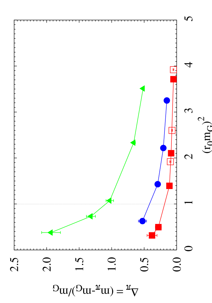
Figure 1: Flavor symmetry violation with the standard thin (triangles), Asqtad (circles) and HYP (filled squares) staggered fermions on $a=0.17$fm quenched configurations. The open squares correspond to dynamical HYP data at similar lattice spacing. The vertical line at $(r_{0}m_{G})^{2}=1$ correspond to $m_{G}\approx 400$MeV pions.

The effect of smearing on flavor symmetry is illustrated in Figure 1 where the relative split between the Goldstone pion $m_{G}$ and lightest non-Goldstone pion $m_{\pi}$

$$\Delta_{\pi}=\frac{m_{\pi}-m_{G}}{m_{G}}$$ (3)

is plotted as the function of the square of the Goldstone pion mass measured in units of $r_{0}$ [17]. The triangles, circles and filled squares in Figure 1 are results obtained with the standard thin link, Asqtad and HYP fermion actions on $8^{3}\times 24$, $\beta=5.7$ Wilson plaquette gauge configurations with lattice spacing $a\approx 0.17$fm. The open squares correspond to dynamical HYP configurations at similar lattice spacing. They agree with the quenched HYP data, indicating that improvement seen in quenched simulations carry over to dynamical ones. For all mass values the HYP action has about an order of magnitude smaller flavor symmetry violations than the standard thin link action, and it is about a factor of two better than Asqtad fermions. It is an interesting question why HYP fermions have better flavor symmetry restoration than Asqtad fermions. Both are perturbative tree level improved, but the HYP links have three levels of SU(3) projections and more gauge loops at each level. Whether it is the SU(3) projection, the extra gauge loops, or both, that make HYP fermions better is not obvious. Recently it has been shown [18] that actions with projected SU(3) links that have the same tree level $O(a^{2})$ improvement are also equivalent at 1-loop level. If that perturbative statement holds true non-perturbatively as well, one could argue that the SU(3) projection is the key to the improved flavor symmetry of the HYP action. The non-perturbative assumption can be easily tested either by quenched measurements of flavor symmetry with projected Asqtad/Fat7 actions or by simply measuring the distribution of the tail of the plaquette with these actions.

2.2 Perturbative Properties of Smeared Actions

A frequent criticism toward smeared (or, for that matter, any kind of improved) actions is that their perturbative properties are not known. This excuse has always been a weak one, and now, that several papers have been published showing that perturbative calculations with smeared links, even projected ones, are doable, the criticism now longer holds. Rather, one should ask if the perturbative properties of smeared actions are better or worse than the standard thin link actions. One can recall that with thin link actions, both with staggered and Wilson fermions, the 1-loop perturbative matching factors for most physically interesting quantities are large. That makes the connection between the lattice and continuum schemes like $\overline{MS}$ unreliable. It has been observed that in the case of staggered fermions the perturbative contribution from the fermion doublers is as large as from the usual gluon tadpoles [19]. Since smearing removes the fermion doublers, it should also improve the perturbative matching factors. Several recent works showed that this is indeed what happens [15, 20, 18, 21]. For example in [21] the 1-loop matching coefficients for several staggered bilinear operators were calculated for different smeared actions. These matching coefficients connect continuum to lattice as

$$O^{\rm{cont}}_{i} \!\!=\!\! O_{i}^{\rm{latt}}\big{(}1+\frac{C_{F}g^{2}}{16\pi^{2}}(2d_{i}ln(\mu a)+c_{i,i})\big{)}$$

$$+\rm{off-diagonal\quad terms}.$$

If a coefficient $c_{i,i}\!\approx 5$ at $1/a=2$GeV lattice spacing, the 1-loop perturbative corrections are about 10%. Table 1 shows the scalar-scalar coefficient that is relevant for the fermionic condensate for the standard thin link, Asqtad and HYP actions. Obviously both the Asqtad and HYP actions satisfy the minimum requirement $c_{1,1}<5$, their matching factors are 10-30 times smaller than the thin link value.

action	Thin link	Asqtad	HYP
$c_{1,1}$	-29.3	-2.2	-0.6

Table 1: The perturbative matching factors for the scalar-scalar bilinear for the standard thin link, Asqtad and HYP fermions [20, 21]

The HYP value is even small enough to use on rougher, $1/a=1.2$GeV configurations where one finds

$$\Sigma(2GeV)_{\overline{MS}}=\frac{1}{Z_{P/S}}\Sigma_{\rm{latt}}(1/a=1.2\rm{GeV}),$$ (5)

with

$$Z_{P/S}=0.92.$$ (6)

This perturbatively determined renormalization Z factor agrees with the value obtained via the non-perturbative matching method of [22]. I will discuss that further in Sect. 4.

3 DYNAMICAL SIMULATIONS WITH SMEARED ACTIONS

Smeared actions that are linear in the thin gauge links, like the Asqtad action, can be simulated with the usual molecular dynamics based algorithms. Calculating the fermionic force for these actions, while tedious, is straightforward. The only problem observed with these simulations is the unusually large autocorrelation time for the topological charge [23].

Actions with projected smeared links, like the HYP action, can not be simulated using molecular dynamics methods as the fermionic force is prohibitively expensive to evaluate. However these actions are smooth enough in the gauge fields to be simulated using a modified version of the well known pseudo-fermion algorithm, the partial-global stochastic metropolis or PGSM update [3, 4, 11, 12]. The PGSM algorithm satisfies the detailed balance condition [24], and with smeared link fermions it can be an efficient algorithm.

We consider a smeared link action of the form

$$S=S_{g}(U)+\bar{S}_{g}(V)+S_{f}(V),$$ (7)

where $S_{g}(U)$ and $\bar{S}_{g}(V)$ are pure gauge actions depending on the thin links $\{U\}$ and smeared links $\{V\}$, respectively, and $S_{f}$ is the fermionic action depending on the smeared links only.The smeared links are constructed deterministically, like hypercubic (HYP) blocking. Any gauge action can be used for $S_{g}(U)$ while $\bar{S}_{g}(V)$ is chosen to optimize the algorithm. The fermionic action describing $n_{f}$ degenerate flavors of staggered fermions is

$$S_{f}(V)=-\frac{n_{f}}{4}\ln\,\mathop{\hbox{Det}}\,\Omega(V)$$ (8)

with $\Omega=M^{\dagger}M$ defined on even sites only. In the PGSM update first a subset of the thin links $\{U\}$ are updated and a new thin gauge link configuration $\{U^{\prime}\}$ is proposed with transition probability that satisfies detailed balance with $S_{g}(U)$. The proposed configuration is accepted with the probability

$$P_{\rm{acc}}=\rm{min}\{1,e^{-\Delta\bar{S}_{g}}e^{-\xi^{*}[A-1]\xi}\},$$ (9)

where $\Delta\bar{S}_{g}=\bar{S}_{g}(V^{{}^{\prime}})-\bar{S}_{g}(V)$ is the difference in the smeared gauge actions, $A=\Omega^{{}^{\prime}-n_{f}/8}\Omega^{n_{f}/4}\Omega^{{}^{\prime}-n_{f}/8}$, and the stochastic vector $\xi$ is generated with Gaussian distribution. In Eq. 9 only one stochastic vector is used in each update step, the acceptance probability approximates the ratio of the old and new actions

$$e^{-\Delta\bar{S}_{g}}\mathop{\hbox{Det}}\,^{n_{f}/4}\Omega^{{}^{\prime}}\Omega^{-1}=e^{-\Delta\bar{S}_{g}}<e^{-\xi^{*}[A-1]\xi}>$$ (10)

only on average. If the stochastic formula estimates this ratio poorly, the autocorrelation time of the update will be large, it could even be infinite. This can be seen if we consider the standard deviation of the stochastic estimator

$$\mathop{\hbox{det}}\,^{-1}(A)=<e^{-\xi^{*}[A-1]\xi}>_{\xi},$$ (11)

$$\sigma_{A}^{2} = <e^{-2\xi^{*}[A-1]\xi}>-<e^{-\xi^{*}[A-1]\xi}>^{2}$$ (12)

$$= \mathop{\hbox{det}}\,^{-1}(2A-1)-\mathop{\hbox{det}}\,^{-2}(A).$$

Eq. 12 is valid only if the matrix $2A-1$ is positive definite. If the matrix $A$ has even one eigenvalue that is less than or equal to 1/2, the formula in Eq. 12 is not valid, the standard deviation is infinite. Unfortunately this is frequently the case as the eigenvalues of the fermionic matrices $\Omega$ and $\Omega^{{}^{\prime}}$ vary from $1/4m^{2}$ to above 16.

There are several ways to improve the efficiency of the stochastic estimator [4]. Here I mention only one, the determinant breakup. If we rewrite the fermionic action of Eq. 8 as

$$S_{f}(V)=-\ln\,\mathop{\hbox{Det}}\,^{n_{f}n_{b}/4}\,\Omega(V)^{1/n_{b}}$$ (13)

with $n_{b}$ an arbitrary integer, the fermionic determinant can be estimated using $n_{b}n_{f}/4$ random source vectors as

$$\mathop{\hbox{det}}\,^{-1}(A)=<e^{-\sum^{n_{b}n_{f}/4}_{i=1}\xi_{i}^{*}[\tilde{A}-1]\xi_{i}}>_{\xi_{i}}$$ (14)

with $\tilde{A}=\Omega^{{}^{\prime}-n_{f}/8n_{b}}\Omega^{n_{f}/4n_{b}}\Omega^{{}^{\prime}-n_{f}/8n_{b}}$. Now the standard deviation is finite as long as none of the eigenvalues of $A$ is less than $1/2^{n_{b}}$, a condition that is much easier to satisfy. In fact for every finite quark mass it is possible to choose $n_{b}$ such that the condition is satisfied. The determinant breakup reduces the statistical fluctuations of the stochastic estimator by taking the sum of $n_{b}n_{f}/4$ smaller terms instead of the original term

$$-\xi^{*}[A-1]\xi\longrightarrow-\sum^{n_{b}n_{f}/4}_{i=1}\xi_{i}^{*}[\tilde{A}-1]\xi_{i}.$$ (15)

While taking the average of several stochastic estimates in the acceptance step of the original PGSM algorithm (Eq. 9) would violate the detailed balance condition, the determinant breakup procedure is still exact.

An added bonus of the determinant breakup is that now simulating arbitrary number of degenerate or non-degenerate flavors is straightforward as long as $n_{b}$ is chosen to be a multiple of 4.

With the determinant breakup of Eq. 14 the acceptance probability can be close to the theoretical maximum, $e^{-\Delta\bar{S}_{g}}\mathop{\hbox{Det}}^{n_{f}/4}\Omega^{{}^{\prime}}\Omega^{-1}$. The PGSM update will be effective only if this value is close to one, i.e. the proposed configurations $\{U\}\longrightarrow\{U^{\prime}\}$ in the first step of the algorithm are close to the dynamical configurations of $S$. Fairly good agreement can be achieved if we choose $S_{g}(U)$ such that it matches the average plaquette and/or correlation length of the dynamical configurations. That requires the shift of the pure gauge coupling that can be compensated by the second pure gauge action term, $\bar{S}_{g}(V)$. Since this term depends on the smeared links, its fluctuations are greatly suppressed and including this term in the acceptance rate does not change it significantly.

The fractional powers of the fermionic matrices in $\tilde{A}$ can be evaluated using polynomial approximation [25, 26], but to evaluate the acceptance probability according to Eq. 14 requires $n_{b}n_{f}/4$ multiplication with $\tilde{A}$, a considerable computational overhead. A detailed study of the autocorrelation of the PGSM update can be found in [4]. Figure 2 shows the cost, measured in $M^{\dagger}M$ matrix multiplies, of creating statistically independent configurations that are separated by two autocorrelation time lengths as the function of the number of links changed in $\{U\}$ to create $\{U^{{}^{\prime}}\}$ in the first step of the PGSM algorithm. The data was obtained with $n_{f}=2$ flavors of dynamical HYP fermions on $8^{3}\times 24,$ about 10fm⁴ volume configurations with different determinant breakup parameters ($n_{b}=8,12$) and quark masses corresponding to $m_{\pi}/m_{\rho}\approx 0.7$ and 0.55. In case of the heavier quark mass the optimal update touches about 4000 links or around 10% of the total links on this volume. With an acceptance rate of 50%, $2\times 10^{5}$ $M^{\dagger}M$ multiplies are needed to create statistically independent configurations. For comparison, creating independent configurations with the standard thin link staggered action at similar lattice spacing at $m_{\pi}/m_{\rho}\approx 0.7$ would require about $6-8\times 10^{5}$ matrix multiplies, a few times more than with the HYP action using the PGSM algorithm.

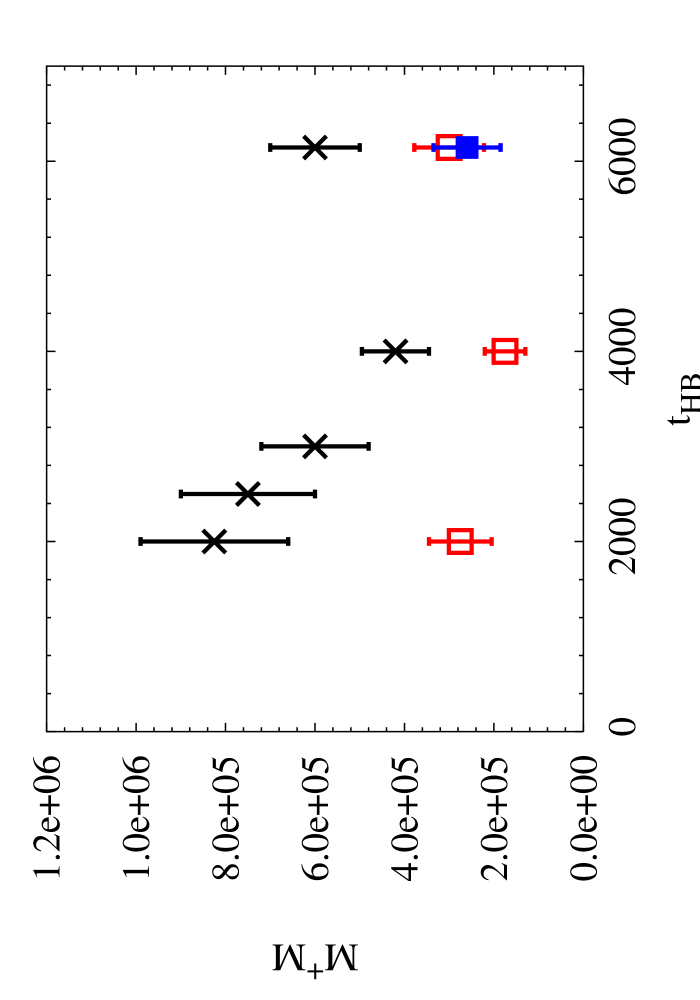
Figure 2: Cost of creating independent configurations with $n_{f}=2$ flavor HYP action, measured in fermionic matrix multiplies. Results are from 10fm⁴ lattices with lattice spacing $a\approx 0.17$fm. Open squares: $n_{b}=8$, $m_{\pi}/m_{\rho}\approx 0.7$, filled square: $n_{b}=12$, $m_{\pi}/m_{\rho}\approx 0.7$, crosses: $n_{b}=12$, $m_{\pi}/m_{\rho}\approx 0.55$ simulations.

The PGSM algorithm is a volume square algorithm. Creating independent configurations on larger volumes will become more and more expensive. However, judging from Figure 2, the computational cost of creating even 100-200fm⁴ configurations is not more than 5-10 times more expensive than molecular dynamics update of thin link staggered fermions.

4 SIMULATION RESULTS WITH HYP FERMIONS

The results summarized in this section are preliminary, obtained on modest size lattices at large lattice spacing with limited computational resources. They are in no way comparable to the extensive data collected with the Asqtad action over the last couple of years, some of it reported at this conference [2, 27]. My goal in this section is to show that the PGSM method is applicable, and at least for standard quantities, nothing unexpected is seen with the HYP action.

Simulations with the HYP action were performed on $8^{3}\times 24$ lattices with $a\approx 0.17$fm lattice spacing with three quark masses corresponding to roughly $m_{\pi}/m_{\rho}=0.7,$ 0.65 and 0.55. To monitor finite size effects and to study the scaling of the algorithm the simulations were repeated on $12^{3}\times 36$ lattices with the two smaller quark mass values. While no autocorrelation time measurement is available on the larger lattices, other factors indicate that the algorithm scales with the square of the volume, maybe even better when comparing the small $8^{3}\times 24$ lattices to the larger volume.

In Figure 1 I have already showed that flavor symmetry restoration with the dynamical HYP action is consistent with the quenched result. Figure 3 shows the scaling of the Goldstone pion mass squared with the quark mass, both measured in units of $r_{0}$. The large finite volume distortion on the smaller volumes is surprising at first, quenched simulations with similar $m_{\pi}/m_{\rho}$ ratios and volumes do not show such effect. However the data is actually consistent with finite volume chiral perturbative calculations [28, 29]. According to these calculations finite volume corrections of the data above are expected to be a few percent on the smaller volume with the largest quark mass and also on the larger volume with the smallest quark mass, larger for the other data points on the smaller volume. Using data with small finite volume corrections we can estimate the renormalization factor $Z_{P/S}$ based on the non-perturbative method of [22]. The value we obtain is consistent with the perturbative prediction in Sect. 2.2

$$Z_{P/s}=0.92(1)\qquad\rm{(non-perturbative)}.$$ (16)

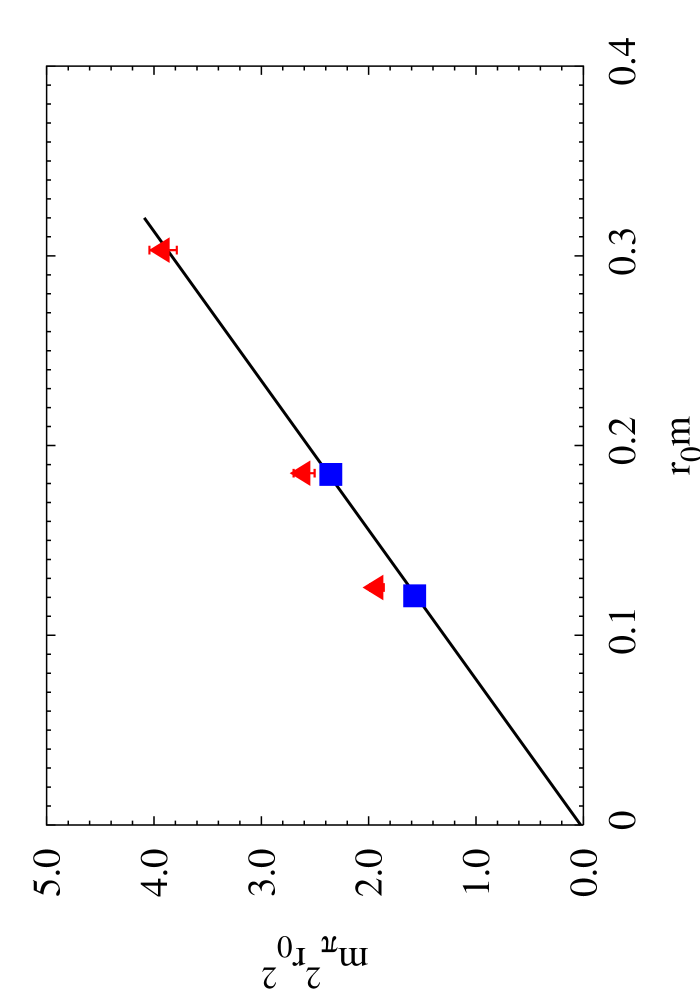
Figure 3: The Goldstone pion mass squared as the function of the quark mass, in units of $r_{0}$. Triangles: $8^{3}\times 24$, squares: $12^{3}\times 36$ lattices, all with $r_{0}\sim 3.0$.

Can we see chiral logarithms in this data? Figure 4 shows the ratio $m^{2}_{\pi}/m_{q}$ as the function of the quark mass, again in units of $r_{0}.$ The data points with small finite volume corrections are consistent with a constant value, at these quark masses there is no obvious sign for chiral logarithms. We can use this data to predict the chiral condensate $\Sigma$ through the GMOR relation. With the renormalization factor obtained above the chiral condensate, translated to $\overline{MS}$ scheme at 2GeV is predicted to be

$$\Sigma_{\overline{MS}}(2GeV)r^{3}_{0}=0.36(4).$$ (17)

This value, though with large errors, seems to be larger than the quenched value $\Sigma^{Quen}_{\overline{MS}}(2GeV)r^{3}_{0}=0.30(4)$ predicted by several groups using a much more sophisticated finite volume method that can be applied only with exactly chiral fermions [30, 22, 31]. The difference between the quenched value and Eq. 17 could be only numerical accuracy, though one would expect a larger condensate from dynamical simulations. New results at smaller lattice spacing and larger volumes can resolve this question in the near future.

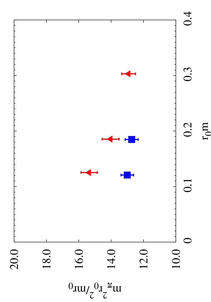
Figure 4: $m^{2}_{\pi}/m$ as the function of the quark mass, in units of $r_{0}$. Notation is the same as in Figure 3.

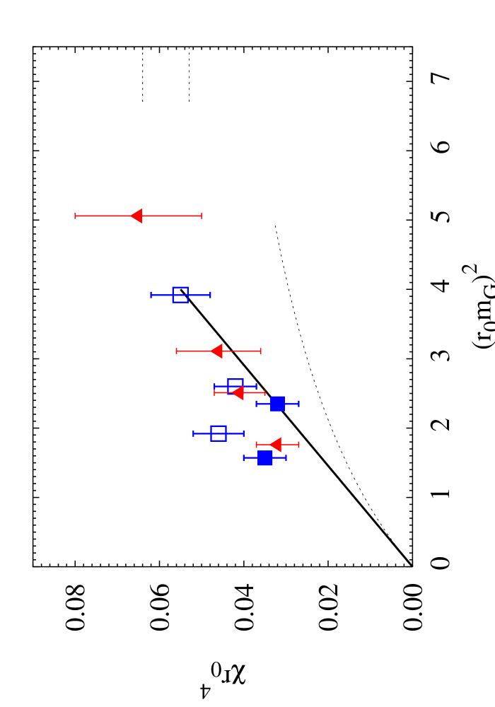
Figure 5: The topological susceptibility as the function of the Goldstone pion mass squared, in units of $r_{0}.$ Triangles: standard thin link staggered fermions at $a\approx 0.10$fm [32]; open squares: HYP action on $8^{3}\times 24$ lattices, $a\approx 0.17$fm; filled squares: HYP action on $12^{3}\times 24$ lattices, $a\approx 0.17$fm. The dashed curve is the prediction from [33], the short lines on the right indicate the quenched value.

I conclude this section with some recent results on the topological susceptibility with HYP fermions. At small quark masses the topological susceptibility is expected to scale linearly with the square of the Goldstone pion mass with a coefficient that is predictable from chiral perturbation theory (solid line in Figure 5). Higher order corrections might push the value even lower (dashed curve in Figure 5) [33]. Numerical simulations have a hard time reproducing this behavior, especially at small quark masses and large lattice spacing, even with improved fermions [32, 23]. In Figure 5 I show results that were obtained with thin link staggered fermions at $a\approx 0.1$fm lattice spacing and with HYP fermions at $a\approx 0.17$fm lattice spacing. The topological charge was measured after 2-3 levels of HYP smearing using an improved topological charge operator [34]. The difference between the smaller and larger volume results with HYP fermions is mainly due to the change of $r_{0}$ and $m_{\pi}$ due to finite volume effects. The topological susceptibility is quite independent of the volume. While even HYP fermions do not reproduce the theoretical expectations, they seem to be consistent with the thin link action results at 70% smaller lattice spacing. It is unlikely that the difference between the numerical results and theoretical expectations are due to the remnant flavor symmetry violations. Even the heaviest of the non-Goldstone pions would predict a smaller topological susceptibility than the measured value at the smallest quark mass. The resolution to this problem might come from exploring the difference of what objects the fermions identify as instantons versus what objects the gluonic charge operators identify as instantons in these simulations.

5 CONCLUSION

Smeared gauge links remove short scale vacuum fluctuations, improving the flavor symmetry of staggered fermion actions. In addition to improved flavor symmetry, smeared fermion actions have improved perturbative properties, like 10-30 times reduced 1-loop matching factors. While these actions are more complicated than thin link ones, with the newly developed partial-global stochastic Metropolis (PGSM) update even SU(3) projected actions can be simulated on fairly large volumes. There are already extensive numerical data with the dynamical Asqtad action using the molecular dynamics based R algorithm. The HYP action has been used in exploratory studies only with the PGSM algorithm.

Many of the properties of the smeared staggered actions should apply to Wilson like fermions as well. Smearing could improve chiral symmetry, and reduce the occurrence of exceptional configurations. Smeared actions also require smaller clover coefficients. In domain wall fermions smearing can reduce the residual chiral symmetry breaking while for overlap fermions smearing increases computational efficiency. These properties are worth exploring in the future.

References

- [1] D. Toussaint, Nucl. Phys. Proc. Suppl. 106 (2002) 111, hep-lat/0110010.
- [2] C. Bernard et al., (2002), hep-lat/0208041.
- [3] A. Hasenfratz and F. Knechtli, Comput. Phys. Commun. 148 (2002) 81, hep-lat/0203010.
- [4] A. Alexandru and A. Hasenfratz, (2002), hep-lat/0207014.
- [5] T. DeGrand, A. Hasenfratz and T.G. Kovacs, Nucl. Phys. B547 (1999) 259, hep-lat/9810061.
- [6] MILC, T. DeGrand, Phys. Rev. D63 (2001) 034503, hep-lat/0007046.
- [7] C. Gattringer, (2002), hep-lat/0208056.
- [8] BGR, C. Gattringer et al., (2002), hep-lat/0209099.
- [9] C.W. Bernard et al., Nucl. Phys. Proc. Suppl. 94 (2001) 346, hep-lat/0011029.
- [10] A. Hasenfratz and F. Knechtli, Phys. Rev. D64 (2001) 034504, hep-lat/0103029.
- [11] A. Hasenfratz and A. Alexandru, Phys. Rev. D65 (2002) 114506, hep-lat/0203026.
- [12] A. Hasenfratz and A. Alexandru, (2002), hep-lat/0209071.
- [13] G.P. Lepage, Phys. Rev. D59 (1999) 074502, hep-lat/9809157.
- [14] MILC, K. Orginos, D. Toussaint and R.L. Sugar, Phys. Rev. D60 (1999) 054503, hep-lat/9903032.
- [15] HPQCD, H.D. Trottier, G.P. Lepage, P.B. Mackenzie, Q. Mason and M.A. Nobes, Nucl. Phys. Proc. Suppl. 106 (2002) 856, hep-lat/0110147.
- [16] A. Hasenfratz, R. Hoffmann and F. Knechtli, (2001), hep-lat/0110168.
- [17] R. Sommer, Nucl. Phys. B411 (1994) 839, hep-lat/9310022.
- [18] W.j. Lee, (2002), hep-lat/0208032.
- [19] M. Golterman, Nucl. Phys. Proc. Suppl. 73 (1999) 906, hep-lat/9809125.
- [20] W.j. Lee and S.R. Sharpe, (2002), hep-lat/0208036.
- [21] W.j. Lee and S.R. Sharpe, (2002), hep-lat/0208018.
- [22] P. Hernandez, K. Jansen, L. Lellouch and H. Wittig, JHEP 07 (2001) 018, hep-lat/0106011.
- [23] MILC, C. Bernard et al., (2002), hep-lat/0209050.
- [24] M. Grady, Phys. Rev. D32 (1985) 1496.
- [25] I. Montvay, Comput. Phys. Commun. 109 (1998) 144, hep-lat/9707005.
- [26] A. Alexandru and A. Hasenfratz, (2002), hep-lat/0209070.
- [27] MILC, C. Bernard et al., (2002), hep-lat/0209079.
- [28] S.R. Sharpe and N. Shoresh, Phys. Rev. D64 (2001) 114510, hep-lat/0108003.
- [29] MILC, C. Bernard, Phys. Rev. D65 (2002) 054031, hep-lat/0111051.
- [30] MILC, T. DeGrand, Phys. Rev. D64 (2001) 117501, hep-lat/0107014.
- [31] P. Hasenfratz, S. Hauswirth, T. Jorg, F. Niedermayer and K. Holland, (2002), hep-lat/0205010.
- [32] A. Hasenfratz, Phys. Rev. D64 (2001) 074503, hep-lat/0104015.
- [33] S. Durr, Nucl. Phys. B611 (2001) 281, hep-lat/0103011.
- [34] T. DeGrand, A. Hasenfratz and T.G. Kovacs, Nucl. Phys. B505 (1997) 417, hep-lat/9705009.