Charmonium at finite temperature in quenched lattice QCD

Abstract

We study charmonium correlators in pseudoscalar and vector channels at finite temperature using lattice QCD simulation in the quenched approximation. Anisotropic lattices are used in order to have sufficient numbers of degrees of freedom in the Euclidean temporal direction. We focus on the low energy structure of the spectral function, corresponding to the ground state in the hadron phase, by applying the smearing technique to enhance the contribution to the correlator from this region. We employ two analysis procedures: the maximum entropy method (MEM) for the extraction of the spectral function without assuming a specific form, to estimate the shape of the spectral function, and the standard $\chi^{2}$ fit analysis using typical forms in accordance with the result of MEM, for a more quantitative evaluation. To verify the applicability of the procedures, we first analyze the smeared correlators as well as the point correlators at zero temperature. We find that by shortening the $t$-interval used for the analysis (a situation inevitable at $T>0$) the reliability of MEM for point correlators is lost, while it subsists for smeared correlators. Then the smeared correlators at $T\simeq 0.9T_{c}$ and $1.1T_{c}$ are analyzed. At $T\simeq 0.9T_{c}$, the spectral function exhibits a strong peak, well approximated by a delta function corresponding to the ground state with almost the same mass as at $T=0$. At $T\simeq 1.1T_{c}$, we find that the strong peak structure still persists at almost the same place as below $T_{c}$, but with a finite width of a few hundred MeV. This result indicates that the correlators possess a nontrivial structure even in the deconfined phase.

I Introduction

The charmonium systems have been payed much attention as a signal of the QCD phase transition. Due to a change of the interquark potential by thermal effects, the $J/\psi$ mass is expected to decrease when approaching the phase transition Has86 . Above $T_{c}$, the screening of the interquark potential may dissolve the charmonium states, and the resulting $J/\psi$ suppression has been regarded as one of the most important signals for detecting the formation of the plasma state MS86 ; Jpsi:exp ; Jpsi:th .

In principle, lattice QCD simulations can provide information on such excitation modes based on a nonperturbative and model independent framework, since the correlation functions in the Euclidean temporal direction measured on a lattice are related to the real time retarded and advanced Green functions by analytic continuation from a single spectral function AGDF59 ; HNS93 . In practice, however, the extraction of reliable information from numerical data for correlators becomes increasingly difficult as the temperature increases. There are two restrictions on the correlators at finite temperature: the numbers of available degrees of freedom, and the physical extent in the temporal direction. The former can be improved by the use of anisotropic lattices, on which the temporal lattice spacings are finer than the spatial ones HNS93 ; TARO01 ; Ume01 . The latter restriction is, however, physically inevitable and may spoil standard procedures applicable at zero temperature.

Recently, there has been technical progress in the direct extraction of the spectral function from lattice data of correlators NAH99 ; SpF_early . The key role is played by the maximum entropy method (MEM), combined with the singular value decomposition for constructing the functional bases in the space of spectral functions. At zero temperature this technique has reproduced spectra consistent with the standard fit analyses NAH99 ; ODS00 ; WK00 ; CPPACS01a ; Fie02 . Application to systems at finite temperature is, however, not straightforward because of the two restrictions mentioned above AMR02 . In particular, shortness of temporal extent, $1/T$, makes it difficult to extract the correct low energy structure of the spectral function. Therefore, one at least needs to verify at $T=0$ that the method produces results which are stable against variation of the $t$-interval. There have already been a number of applications of MEM for finite temperature Bielefeld02a ; Bielefeld02b ; Bielefeld02c ; AHN02 , but as long as such tests are not systematically performed these results may contain uncontrolled uncertainties. In fact, we will show in this paper that MEM applied to point-point correlators at $T=0$ with shortened $t$-interval fails to produce the correct spectral functions. We therefore apply the smearing technique to enhance the contribution of the low energy part to the correlators ODS00 ; TARO01 ; Ume01 . For the smeared correlators at $T=0$, MEM works, at least qualitatively, also with a shorter $t$-interval.

In this paper, charmonium correlators are investigated using lattice QCD simulations in the quenched approximation. We focus on properties of the ground state, more generally the low energy structure of the correlator, rather than the whole spectral function. This paper mainly deals with the following two subjects:

(1) A technical investigation of procedures for extraction of reliable information from the numerical data of correlators in the temporal direction. In addition to MEM, we apply the standard $\chi^{2}$ fit analysis assuming a peak structure for the spectral function ISM02 . The latter approach complements the former, since MEM with small numbers of data points appears not work beyond the level of qualitative estimate for the shape of spectral function.

(2) A study of temperature effects on the correlators near to the deconfining phase transition. Below $T_{c}$, the question is whether the charmonium mass shifts, as expected from the potential model approach Has86 . Above $T_{c}$, previous studies have indicated that nontrivial structures may survive TARO01 ; Ume01 . The possibility of the existence of collective modes in the plasma phase is therefore carefully examined.

We use quenched anisotropic lattices with the renormalized anisotropy $\xi=a_{\sigma}/a_{\tau}=4$ and the spatial lattice cutoff $a_{\sigma}^{-1}\simeq 2$ GeV. The phase transition occurs near $N_{t}=28$, and hence sufficiently many points are available in the vicinity of $T_{c}$. At $T\simeq 0$ we try to determine the conditions for a reliable extraction of the spectral function. We find that for the point correlators, reliability of MEM with less than 24 $t$-points (meaning a physical $t$-range of less than $O(0.5\mbox{fm})\sim 0.7T_{c}$) is not guaranteed with the present level of statistics. Therefore only the smeared correlators are analyzed at finite temperature, $T\simeq 0.9T_{c}$ and 1.1 $T_{c}$.

Here we comment on the smearing technique. Although the correlator of spatially extended operators has no direct relation to the physically observable dilepton production rate, the properties of collective excitations such as mass and width are unchanged and can be probed more efficiently. To the extent that these excitations drive the dilepton rate we can at least say something about their position and shape, if not about their strength. A disadvantage is the possibility of detecting a fake peak, which may be produced by the smearing even in the case of free quarks Bielefeld02a . To distinguish such an artifact from a genuine physical peak we use besides the smearing function based on the wave function obtained at $T=0$ also a narrower one of essentially half-width. We speak thereby of “smeared” and of “half-smeared” correlators (because the energy region enhanced by this narrower smearing function is wider, while the high frequency part of $O(1/a_{\tau})$ is still sufficiently suppressed). Comparing the results of these two types of smeared correlators, one can argue whether the observed peak structure is an artifact of free quarks or physical indication of a collective mode.

This paper is organized as follows. In Sec. II, we recall some fundamental properties of the spectral function. For later uses in the $\chi^{2}$ fit analysis, presumable forms of the spectral function for a collective mode are discussed. Section III reviews anisotropic lattice actions and describes the parameters used in this paper. We also show the spectral function of the correlator of a free quark-antiquark pair, for comparison with the correlators from the Monte Carlo simulation. In Sec. IV our analysis procedures are explained. Section V describes the setup of Monte Carlo simulation. The following three sections show the result of the numerical simulation. In Section VI we analyze the correlators at zero temperature, as a preparation for the more involved situations at finite temperatures. Sections VII and VIII show the results at $T\simeq 0.9T_{c}$ and $1.1T_{c}$, respectively. In each case, we first estimate the presumable form of the spectral function with MEM, and then apply the $\chi^{2}$ fit analysis for a more quantitative evaluation of its structure. Section IX is devoted to our conclusions on the technical and physical implications of the results. Our preliminary results have been reported in Ref. NMUM02 .

II Spectral function

In this section $\beta$ represents the inverse temperature and should not be confused with the coupling of gauge field which appears in later sections. For a finite lattice of temporal extent $N_{\tau}$ we have $\beta=1/T=N_{t}a_{\tau}$. The Euclidean time is represented by $\tau$ in this section to make clear the distinction between the Euclidean and Minkowski formulations. In later sections we use also $t$ as the Euclidean time, because no confusion is expected for the lattice QCD formulated in the Euclidean space.

We consider correlators of the form:

$$C(\tau)=\sum_{\vec{x}}\langle O(\vec{x},\tau)O^{{\dagger}}(0,0)\rangle,$$ (1)

where the operator $O(\vec{x},\tau)$ is a quark bilinear,

$$O(\vec{x},\tau)=\sum_{\vec{y}}\phi(\vec{y})\bar{q}(\vec{x}+\vec{y},\tau)\Gamma q(\vec{x},\tau).$$ (2)

4$\times$4 matrix $\Gamma$ specifies the quantum number, such as, for example, $\Gamma=\gamma_{5}$ for pseudoscalar and $\gamma_{i}$ ($i=1,2,3$) for vector channels. $\phi(\vec{y})$ is a smearing function defining the spatial extension of the bilinear operator. Since the smearing in general violates the gauge invariance of the correlator, one needs to fix the gauge or employ a gauge invariant form of the smearing function. We fix the configurations to the Coulomb gauge, since it is widely used and allows easy implementation of the smearing function. Source and sink operators are always identical in this work.

Point correlators correspond to a ultra local “smearing function” $\phi(\vec{y})=\delta_{\vec{y},0}$ in Eq. (2). For the smeared correlators we use smearing function of the form

$$\phi(\vec{y})=\exp(-a|\vec{y}|^{p}),$$ (3)

where the parameters $a$ and $p$ are determined by fitting the wave function measured in the numerical simulation to the above form. The smearing technique described here was already applied to the problems of the charmonium correlators at $T>0$ Ume01 , as well as to the light meson correlators TARO01 .

For a while let us consider the continuum Euclidean space. The Matsubara Green function is represented in terms of the spectral function as

$$G(\nu_{n},\vec{p})=\int_{-\infty}^{\infty}\frac{d\omega}{2\pi}\frac{\rho(\omega,\vec{p})}{i\nu_{n}-\omega+i\epsilon}.$$ (4)

The spectral function $\rho(\omega,\vec{p})$ is represented as

$$\rho(\omega,\vec{p}) = \frac{1}{2Z(\beta)}\sum_{n,m}(e^{-\beta E_{n}}-e^{-\beta E_{m}})|\langle n|O(0)|m\rangle|^{2}$$ (5)

$$\times(2\pi)^{4}\delta(\omega-E_{m}+E_{n})\delta(\vec{p}-\vec{P}_{m}+\vec{P}_{n}),$$

which is an odd real function due to the bosonic nature of the present correlator and positive for $\omega>0$.

The retarded and advanced Green functions for real time are represented as

$$G^{R}(\nu,\vec{p}) = \int_{-\infty}^{\infty}\frac{d\omega}{2\pi}\frac{\rho(\omega,\vec{p})}{\nu-\omega+i\epsilon}$$ (6)

$$G^{A}(\nu,\vec{p}) = \int_{-\infty}^{\infty}\frac{d\omega}{2\pi}\frac{\rho(\omega,\vec{p})}{\nu-\omega-i\epsilon}$$ (7)

with the same spectral function, $\rho(\omega,\vec{p})$ AGDF59 . The spectral function is then represented as

$$\rho(\nu,\vec{p})=-2\;\mbox{Im}G^{R}(\nu,\vec{p})=2\;\mbox{Im}G^{A}(\nu,\vec{p}).$$ (8)

Strictly speaking, the above integrations do not always converge, and one needs appropriate subtraction terms. On the other hand, the high frequency part of the spectral function is not practically significant in the numerical analysis, because of the strong suppression by $K(\tau,\omega)$, and of the existence of the lattice cutoff. We therefore do not consider these subtractions in this paper. We note that the smearing of the operator in Eq. (2) is performed only in the spatial directions, and therefore the analytic continuation of the Matsubara Green function to the real time Green functions is independent of this operation (but, of course, the spectral function depends on the operators, hence on smearing).

In the following we are only concerned with the correlators projected on the zero momentum states and discard the argument $\vec{p}$. Since the spectral function $\rho(\omega)$ is an odd function in $\omega$, the correlator (1) is represented as

$$C(\tau)=\int_{0}^{\infty}\frac{d\omega}{2\pi}K(\tau,\omega)\rho(\omega).$$ (9)

where

$$K(\tau,\omega)=\frac{e^{-\omega\tau}+e^{-\beta\omega+\omega\tau}}{1-e^{-\beta\omega}}.$$ (10)

In the numerical simulation of lattice QCD one measures the left hand side of Eq. (9). The question is how to solve the inverse problem to obtain $\rho(\omega)$ with limited data for $C(\tau)$. The procedures to extract information about $\rho(\omega)$ are described in Sec. IV.

Now we shall present several ansätze for the spectral function which will be used for later analysis of the lattice data, and discuss their physical implications. A simple representation of a collective mode is the following form of the retarded Green function:

$$G^{R}(\nu)=\frac{R(\nu)}{\nu-\mu+i\gamma(\nu)/2},$$ (11)

where $\mu$ and $\gamma(\nu)$ express the dispersion and the width of the mode. The corresponding spectral function is the well-known Breit-Wigner form. We shall neglect the frequency dependence of the width $\gamma$ for simplicity. Taking the oddness of the bosonic spectral function into account, $\rho(\omega)$ reads

$$\rho(\omega)=\frac{\gamma R(\omega)}{(\omega-m)^{2}+\gamma^{2}/4}-\frac{\gamma R(\omega)}{(\omega+m)^{2}+\gamma^{2}/4}.$$ (12)

If the quantum numbers of the operators used to represent the collective mode are the correct ones, the physical properties associated with the mode, characterized by $\mu$ and $\gamma$, are independent of the particular operator. Therefore the smeared operators can be used to observe these quantities. However, the smearing does change the overlap of the operator with the state, $R(\omega)$. Therefore the effects depending on $R(\omega)$ and those coming only from the peak structure (represented with $\mu$ and $\gamma$) should be distinguished. If the change of $R(\omega)$ is sufficiently gentle over the region of the observed peak, the $\omega$ dependence in $R(\omega)$ is negligible.

Instead of Eq. (12), at zero temperature one often uses the relativistic Breit-Wigner type form:

$$\rho(\omega)=\frac{\mbox{sign}(\omega)\omega^{2}m\gamma(4R/m)}{(\omega^{2}-m^{2})^{2}+m^{2}\gamma^{2}}.$$ (13)

This form shows a similar behavior to Eq. (12) around the peak position. However, the behavior far from the peak is different. In particular (12) and (13) give different contribution to the integral (9) near vanishing $\omega$: In the vicinity of $\omega=0$, Eq. (12) behaves linearly in $\omega$, while Eq. (13) behaves linearly in $\omega^{2}$. Since $K(\tau,\omega)$ behaves as $(2-\beta\omega)/\beta\omega$, Eq. (12) gives a $t$-independent contribution to the integral (9) AMR02 . We note that there is no indication of linear behavior in $\omega$ in the small $\omega$ region of the spectral functions obtained from our numerical data with MEM, as shown in Sec. VII and VIII. Therefore, in the $\chi^{2}$ fit analysis, we use the form of Eq. (13) as ansatz for the spectral function to which the lattice data are fitted. While the use of Eq. (13) is valid at zero temperature, it should only be taken as a representative form of peak structure at $T>0$, and hence the parameters $m$ and $\gamma$ do not have a strict sense but represent only a convenient parameterization of the peak.

In the limit of $\gamma\rightarrow 0$, both Eqs. (12) and (13) tend towards a delta function form,

$$\rho(\omega)=2\pi R\left[\delta(\omega-m)-\delta(\omega+m)\right].$$ (14)

This form corresponds to the standard exponential fit of correlators used in the hadron spectroscopy at zero temperature.

III Anisotropic lattice QCD

III.1 Anisotropic lattice actions

For analysis of the correlators in the temporal direction at $T>0$ the fine temporal resolution is very important to extract meaningful information TARO01 ; Ume01 ; ISM02 . Anisotropic lattices have become a powerful tool to achieve sufficiently high temporal cutoff while keeping total computational size modest. In the following, we summarize the anisotropic lattice actions employed in this work. The parameters we use are described in the next subsection.

For the gauge field, we adopt the standard Wilson plaquette action Kar82 ,

$$S_{G} = \beta\gamma_{G}\sum_{x}\sum_{i=1}^{3}\left[1-\frac{1}{3}\mbox{ReTr}U_{i4}(x)\right]$$ (15)

$$+\frac{\beta}{\gamma_{G}}\sum_{x}\sum_{i<j=1}^{3}\left[1-\frac{1}{3}\mbox{ReTr}U_{ij}(x)\right],$$

where $U_{\mu\nu}$ is a product of link variables along a plaquette in the $\mu$-$\nu$ plane. Here the parameters $\beta$ and $\gamma_{G}$ are bare coupling and bare anisotropy, respectively.

For the quark field we use the $O(a)$ improved Wilson-type action Ume01 ; Aniso01a ; Aniso01b :

$$S_{q}=\sum_{x,y}\bar{q}(x)K(x,y)q(y),$$ (16)

$$K(x,y) = \delta_{xy}$$ (17)

$$-\kappa_{\tau}\left[(1\!-\!\gamma_{4})U_{4}(x)\delta_{x+\hat{4},y}+(1\!+\!\gamma_{4})U_{4}(x-\hat{4})\delta_{x-\hat{4},y}\right]$$

$$-\kappa_{\sigma}\sum_{i=1}^{3}\left[(r\!-\!\gamma_{i})U_{i}(x)\delta_{x+\hat{i},y}+(r\!+\!\gamma_{i})U_{i}(x\!-\!\hat{i})\delta_{x-\hat{i},y}\right]$$

$$-\kappa_{\sigma}c_{E}\sum_{i=1}^{3}\sigma_{4i}F_{4i}(x)\delta_{x,y}$$

$$-\kappa_{\sigma}c_{B}\sum_{i>j=1}^{3}\sigma_{ij}F_{ij}(x)\delta_{x,y}.$$

where $\kappa_{\sigma}$ and $\kappa_{\tau}$ are the spatial and temporal hopping parameters, respectively, $r$ is the spatial Wilson parameter, and $c_{E}$, $c_{B}$ are the clover coefficients for the $O(a)$ improvement. We set $r=1/\xi$ and $c_{E}$, $c_{B}$ to the tadpole-improved tree-level values, and vary the two parameters $\kappa_{\sigma}$ and $\kappa_{\tau}$ to change the quark mass and the fermionic anisotropy. The tadpole improvement LM93 is performed by rescaling the link variables as $U_{i}(x)\rightarrow U_{i}(x)/u_{\sigma}$ and $U_{4}(x)\rightarrow U_{4}(x)/u_{\tau}$, respectively, with the corresponding mean-field values of the spatial and temporal link variables, $u_{\sigma}$ and $u_{\tau}$. Then $c_{E}$ and $c_{B}$ with the choice $r=1/\xi$ read as

$$c_{E}=1/u_{\sigma}u_{\tau}^{2},\hskip 14.22636ptc_{B}=1/u_{\sigma}^{3}.$$ (18)

Instead of $(\kappa_{\sigma},\kappa_{\tau})$, it is convenient to use the parameters

$$\gamma_{F} \equiv u_{\tau}\kappa_{\tau}/u_{\sigma}\kappa_{\sigma},$$ (19)

$$\frac{1}{\kappa} \equiv \frac{1}{u_{\sigma}\kappa_{\sigma}}-2(\gamma_{F}+3r-4)=2(m_{0}\gamma_{F}+4),$$ (20)

where $m_{0}$ is the bare quark mass in temporal lattice units. $\kappa$ plays the same role as on isotropic lattices, and controls the bare quark mass. $\gamma_{F}$ is the bare fermionic anisotropy.

The lattice quark field $q(x)$ in the action (17) is related to the dimensionful field $\psi(x)$ as

$$\psi(x)=a_{\sigma}^{-3/2}Z_{q}(\beta,\kappa){\cal K}(\kappa)q(x),$$ (21)

where we assume $m_{Q}\ll a_{\tau}^{-1}$. ${\cal K}(\kappa)$ is so-called KLM normalization factor KLM ,

$${\cal K}(\kappa) = [2u_{\tau}\kappa_{\tau}(1+m_{0})]^{1/2}$$ (22)

$$= \left[\frac{1+2\kappa(\gamma_{F}-4)}{1+2\kappa(\gamma_{F}+3r-4)}\right]^{1/2}.$$

We consider the tadpole-improved tree-level matching of the fields in continuum and lattice theories, and hence $Z_{q}$ is set to unity.

III.2 Parameters

We here describe the parameters used in this paper. First, we discuss the calibration of gauge and quark fields. In an interacting theory, the renormalized anisotropy $\xi=a_{\sigma}/a_{\tau}$ generally differs from the bare anisotropy parameters $\gamma_{G}$ and $\gamma_{F}$. Therefore one needs to tune the latter such that

$$\xi_{G}(\gamma_{G},\gamma_{F})=\xi_{F}(\gamma_{G},\gamma_{F})=\xi$$ (23)

holds, where $\xi_{G}$ and $\xi_{F}$ are the observed anisotropies defined through the gauge and fermionic observables, respectively. In quenched simulations, one can calibrate the gauge and fermion fields separately, first the former, and then the latter.

For the calibration of the gauge field, we refer to an elaborated work by Klassen Kla98 which uses Wilson loops in the spatial-spatial and spatial-temporal planes and is performed at 1% accuracy level. Making use of his relation of $\gamma_{G}$ to $\beta$ and $\xi$, we choose $\beta=6.10$ and $\gamma_{G}=3.2108$ corresponding to the renormalized anisotropy $\xi=4$. These values were also adopted in Ref. Aniso01b , and correspond to the spatial lattice cutoff $a_{\sigma}^{-1}=2.030(13)$ GeV set by the hadronic radius $r_{0}$ Som94 .

For the quark field, we use the result of Ref. Aniso01b in which the calibration was performed on the same lattice as this work using the meson dispersion relation in a quark mass region including the charm quark mass. Accordingly, we adopt $\kappa=0.112$ and $\gamma_{F}=4.00$, namely $m_{q}=0.121$, as the values corresponding to the charm quark mass. (In Ref. Aniso02a it was argued that the value of $\gamma_{F}$ tuned for the massless quark is also applicable to the charm quark mass. For historical reason, however, we use the result of the mass dependent tuning in Ref. Aniso01b . The difference is actually small and does not cause any significant effect.)

As smearing function we use the result for the wave function in the Coulomb gauge at $T=0$. For the vector channel the fit to Eq. (3) yields $a=0.2275(9)$ and $p=1.258(5)$. These values are used for both the pseudoscalar and vector correlators.

In addition, we also use a narrower smearing function with $a=0.45$ and the same $p$. The correlators smeared with this function are called half-smeared correlators, since the smearing function has about twice the slope as the main one and hence a smaller smearing effect is expected: the low energy part of the correlator is only partially enhanced, while the high energy part of $O(1/a_{\tau})$ is sufficiently reduced. This intermediate smearing function plays an important role at $T>T_{c}$ in examining whether the observed peak structure of the spectral function for the smeared correlator is an artifact of smearing or a genuine physical effect (Sec. VIII).

III.3 Free quark case

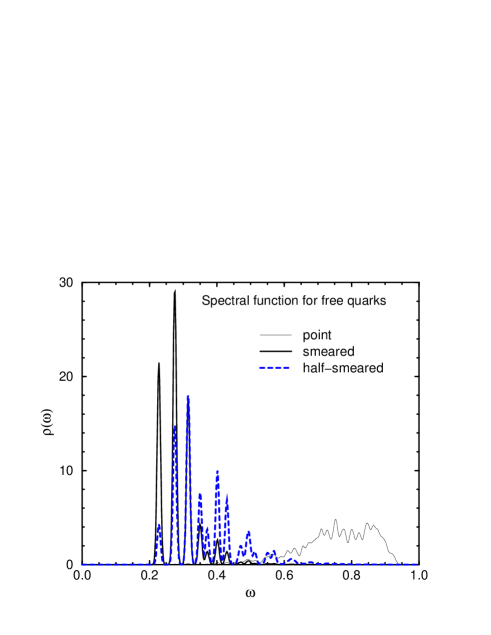
Figure 1: The spectral functions for the pseudoscalar correlators composed of free quarks at $T=0$.

Since in the perturbative plasma regime we expect free quarks and gluons it is important to compare the result of Monte Carlo simulation with the case of free quarks on the lattice. The spectral function of the correlator (1) in the case of free quarks is obtained from the expression (5). In the case of vanishing total momentum, for positive frequency,

$$\rho(\omega) = \frac{\pi}{Z}\sum_{\vec{p}}[1-e^{-N_{t}2E(\vec{p})}]\tilde{\phi}(\vec{p})^{2}$$ (24)

$$\times\sum_{j,k=1,2}\left[\frac{\bar{v}_{j}(-p)\Gamma u_{k}(p)}{2E(p)}\right]^{2}\delta\left(\omega-2E(\vec{p})\right)$$

where $u_{j}(p)$ and $v_{j}(p)$ are the quark and antiquark spinors with $j$-th spin, and $\tilde{\phi}(\vec{p})$ is the Fourier transform of $\phi(\vec{y})$. The summation in $\vec{p}$ is taken over all modes on the finite lattice of the same size as in Monte Carlo simulation, $20^{3}$. With the present lattice quark action, the energy of free quark, $E(\vec{p})$, satisfies the dispersion relation Ume01 ; Aniso01a

$$\cosh E(\vec{p})=1+\frac{\vec{\bar{p}}^{2}+\left[m_{0}+\frac{r}{2\gamma_{F}}\vec{\hat{p}}^{2}\right]^{2}}{2\left[1+m_{0}+\frac{r}{2\gamma_{F}}\vec{\hat{p}}^{2}\right]},$$ (25)

where $\bar{p}_{i}=(1/\gamma_{F})\sin p_{i}$ and $\hat{p}_{i}=2\sin(p_{i}/2)$. We set the bare quark anisotropy $\gamma_{F}=\xi=4$ and the bare quark mass $m_{0}=0.121$ such that the free quark has the same value as in the Monte Carlo simulation.

Figure 1 shows the spectral functions of point, smeared, and half-smeared correlators composed of free quarks in PS channel. The integral of these functions are normalized to unity. Since on the finite lattice the spectral function is a sum of delta functions, we represent each contribution at momentum $\vec{p}$ with a Gaussian of width 0.005. As clearly shown in the figure, the smearing of the operator strongly enhances the low energy part of the spectral function, as compared to the point correlator. In the (fully) smeared correlator, several low momentum states over the range of $\omega$ about 0.1 dominate the correlator. From this correlator, therefore, an analysis with poor energy resolution in $\omega$ might produce a peak with full width of order of 0.1 instead of a sum of distinct peaks corresponding to individual momentum states. As we will see in Sec. IV.4, the $\chi^{2}$ fit analysis with the single Breit-Wigner type ansatz applied to the smeared correlator composed of free quarks produces a much narrower peak with the width of about 0.027 centered at $\omega\simeq 0.275$. This is of the same order of magnitude as the width extracted from the correlators in Monte Carlo simulation at $T\simeq 1.1T_{c}$. Therefore this occasion must be examined carefully.

It is for this purpose that the half-smeared correlator is introduced. As shown in Fig. 1, a slightly higher and wider frequency region contributes dominantly to the half-smeared correlator than to the smeared one. If the correlator is approximated by a single peak, the peak will be centered at larger energy and have wider width as compared to those of the smeared correlator. This behavior is verified in Sec. IV by applying the $\chi^{2}$ fit analysis to the correlators composed of free quarks. Therefore, comparing the results for spectral functions for the smeared and half-smeared correlators can help judging whether the peak observed from the simulation data is a genuine excitation mode or an artifact brought by the smearing.

IV Analysis procedure

IV.1 Strategy of analysis

One of the goals of this work is to investigate techniques to extract the relevant information of the spectral function from the correlators with limited numbers of the degrees of freedom. We treat an inverse problem represented as

$$C(t)=\int_{0}^{\infty}d\omega K(t,\omega)A(\omega),$$ (26)

where $C(t)$ is the given lattice result for the correlator, and the spectral function $A(\omega)$ is what we need to obtain. Hereafter we shall denote the spectral function reconstructed from the lattice data $A(\omega)$ instead of $\rho(\omega)$ ($\times(2\pi)^{-1}$). Unless stated otherwise, the variables are in temporal lattice units in the following. The kernel $K(t,\omega)$ is given as

$$K(t,\omega)=\frac{e^{-\omega t}+e^{-\omega(N_{t}-t)}}{1-e^{-N_{t}\omega}}.$$ (27)

This is the continuum type kernel, and an alternative form of the kernel which explicitly incorporate the lattice structure was also applied in the literatures NAH99 ; Bielefeld02a . We have seen no significant difference in applying the two kernels, therefore we shall not further discuss this point. In practice, the above integration over the frequency $\omega$ is replaced by a summation with sufficiently fine discretization $\Delta\omega$ and a cut off at some maximum value $\omega_{max}$.

As already mentioned, one of the main analysis procedures is the maximum entropy method (MEM) NAH99 . Before applying it to finite temperature problems, one should verify its applicability under the condition which one encounters at $T>0$. For this we test how the result changes when varying the number of data points used in analysis for the correlators at $T=0$. The condition to be satisfied is that the ground state peak – which we know to exist at $T=0$ – is correctly reproduced, at least at a qualitative level. We stress that without such verification, the result of MEM may contain uncontrolled artifacts at finite temperature. Concerning quantitative questions, we find that with reduced number of data points, MEM hardly gives a result beyond the qualitative level, for example for the width of a peak.

Another technique in our hand is the standard $\chi^{2}$ fit assuming a certain ansatz for the spectral function. This method has been applied to a problem of glueballs at finite temperature ISM02 . A disadvantage of this approach is that one needs to assume a form of the spectral function, which introduces a bias. For this purpose, the result of MEM can be a good guide. Once a specific ansatz is used, the $\chi^{2}$ fit gives much more reliable results than MEM for the parameters, both in statistical as well as systematic sense.

Therefore MEM and the $\chi^{2}$ fit are complementary to each other at this stage of computational power, and in combination provide a more reliable way to analyze the structure of spectral functions than taken independently. We thus propose a two-step procedure: we first apply MEM to the correlators, for a rough estimate of the shape of spectral function. Once a presumable form is known, we then examine this form using $\chi^{2}$ fit, and estimate the values of parameters such as the mass and width of a peak structure.

IV.2 Maximum entropy method

Our MEM analysis basically follows Ref. NAH99 , which reviews in detail the maximum entropy method applied to data of lattice QCD simulation. Here we briefly summarize just several formulae necessary for the later description of our analysis.

To obtain $A(\omega)$ from $C(t)$ by solving the inverse problem Eq. (26), the maximum entropy method maximizes a functional

$$Q(A;\alpha)=\alpha S[A]-L[A].$$ (28)

$L[A]$ is the likelihood function,

$$L[A]=\frac{1}{2}\sum_{t_{1},t_{2}}[C(t_{i})-C_{A}(t_{i})]V(t_{i},t_{j})^{-1}[C(t_{j})-C_{A}(t_{j})],$$ (29)

where $C_{A}(t)$ is the resulting correlator (26) for the trial $A(\omega)$, and $V(t_{i},t_{j})$ is the covariance matrix of the data

$$V(t_{i},t_{j})=\frac{1}{N(N\!-\!1)}\sum_{k=1}^{N}\left[C_{k}(t_{i})-C(t_{i})\right]\left[C_{k}(t_{j})-C(t_{j})\right]$$ (30)

with $C_{k}(t)$ the $k$-th sample of the correlator. The standard $\chi^{2}$ fit minimizes this functional $L$. The Shannon-Jaynes entropy $S[A]$ is defined as

$$S[A]=\int_{0}^{\infty}d\omega\left[A(\omega)-m(\omega)-A(\omega)\log\left(\frac{A(\omega)}{m(\omega)}\right)\right].$$ (31)

The function $m(\omega)$ is called the default model, and should be given as a plausible form of $A(\omega)$. The parameter $\alpha$ can be integrated out at the last stage of calculation. Following Ref. NAH99 , we use a form

$$m(\omega)=m_{DM}\omega^{2}.$$ (32)

In the case of point correlators, a natural choice of $m_{DM}$ is determined according to the asymptotic behavior of the meson correlators at large $\omega$ in perturbation theory. Although such an asymptotic behavior is not observed in practical simulation because of the finite lattice cutoff, this form has been successfully applied to problems at zero temperature NAH99 ; CPPACS01a . For the smeared correlators, the situation is more subtle, since the high frequency part of the correlator is suppressed by the smearing function. We therefore adopt a practical choice: we normalize the smeared correlator so as to produce the same overlap with the ground state as the point correlator. Then the same normalization is also applied to the correlators at finite temperatures, and we observe how the result changes with the change of $m_{DM}$.

In the maximization step of $Q(A;\alpha)$ the singular value decomposition of the kernel $K(t,\omega)$ is used. Then the spectral function is represented as a linear combination of the eigenfunctions of $K(t,\omega)$. The number of degrees of freedom of $A(\omega)$ is accordingly reduced to the number of data points of the correlator. Although the coefficients of the linear combination for $A(\omega)$ can in principle be determined uniquely from the data without introducing an entropy term, the small eigenvalues of $K(t,\omega)$, $\theta_{i}$, lead for the spectral function to a singular behavior; hence truncation at some $i$ is practically required SpF_early . In MEM, the addition of the entropy term stabilizes the problem and guarantees an unique solution for the coefficients of the eigenfunctions NAH99 . In our analysis, we use only the basis functions for which $\theta_{i}>10^{-12}\times\theta_{1}$ holds, where $\theta_{i}$ is $i$-th largest singular value. This restriction has no significant effect on the result.

IV.3 $\chi^{2}$ fit with ansatz for the spectral function

The standard $\chi^{2}$ fit method minimizes the likelihood function $L$, Eq. (29), with an assumed form for the spectral function. A most simple form for fit function is the delta function:

$$A_{pole}(\omega;r,m)=r\delta(\omega-m).$$ (33)

This form is referred to as pole ansatz in the following. At $T=0$, a sum of several pole terms should describe well the correlators. For the correlators below $T_{c}$, where narrow thermal widths are expected, the multi-pole form is also convenient to test this assumption.

As noted in Sec. II, to describe a peak structure with finite width we adopt the relativistic Breit-Wigner form (referred to as BW form),

$$A_{BW}(\omega;r,m,\gamma)=\frac{\omega^{2}rm\gamma}{(\omega^{2}-m^{2})^{2}+m^{2}\gamma^{2}}.$$ (34)

This is the same form as Eq. (13), with slightly modified notation for convenience. This ansatz neglects the $\omega$ dependence of $r$, and hence is valid only for the case that the width of the peak, $\gamma$, is sufficiently small compared with the change of the smearing function in the region of interest.

Combining these two forms, we fit the numerical data of correlators to the following ansätze:

2-pole form: this form is suitable for description of correlators at $T=0$. It is also expected to be a good representation of correlators at $T<T_{c}$;

$$A(\omega)=A_{pole}(\omega;r_{0},m_{0})+A_{pole}(\omega;r_{1},m_{1}).$$ (35)

1-BW form: if the contribution from the high frequency part of the spectral function is negligible, a collective excitation at low energy is expected to be well represented by a single Breit-Wigner type ansatz:

$$A(\omega)=A_{BW}(\omega;r_{0},m_{0},\gamma_{0}).$$ (36)

This form is also a good representation for the spectral function of the smeared correlator composed of free quarks.

BW+pole form: although the lowest peak is well represented with the Breit-Wigner type function, there may exist contribution from high frequency region. Since the smearing of operator suppress such contribution, remaining effects of this region may be represented as a single pole-like term. This is the reason that we fit the data to the form

$$A(\omega)=A_{BW}(\omega;r_{0},m_{0},\gamma_{0})+A_{pole}(\omega;r_{1},m_{1}).$$ (37)

This is the most general ansatz for $\chi^{2}$ fit in this paper.

These ansätze form are the basis for the analysis of the lowest peak structure, which corresponds to the ground state at $T<T_{c}$. The structure in the high frequency region is out of the scope of this paper.

IV.4 Analysis of correlators composed of free quarks

Figure 2: The result of MEM analysis for the spectral function from the smeared PS correlator composed of free quarks at $T=0$.

Figure 3: The result of $\chi^{2}$ fit analysis for the spectral functions from the PS correlators composed of free quarks at $N_{t}=26$.

To learn how to distinguish physical features of the correlators from artifacts due to the smearing we apply MEM and the $\chi^{2}$ fit analyses to the correlators composed of free quarks on our lattice, which were discussed in Sec. III.3.

For the MEM analysis, the fluctuations of the correlators are given by hand in the same manner as the mock data analyses in Refs. NAH99 ; CPPACS01a . The deviations of the correlators are less than those of the data from the Monte Carlo simulation. Figure 2 shows the result of MEM applied to the smeared correlator in pseudoscalar channel composed of free quarks at $T=0$. The upper bound of $t$ region used for the analysis, $t_{max}$, is varied to observe how the result of MEM depends on the $t$-region used. With decreasing $t_{max}$, the resolution of the spectral function becomes worse, and for $t_{max}\leq 16$ the spectral function extracted with MEM displays just one peak. Therefore for the circumstances specific at $T>0$ MEM does not have sufficient resolution to distinguish individual states if they are closer than about $0.05a_{\tau}^{-1}$. If the correlator is composed of almost free quarks, the width extracted with MEM may be of order of 0.05–0.1 in temporal lattice units.

We also apply the $\chi^{2}$ fit analysis to the correlators composed of free quarks. In this case the errors of the same size as in Monte Carlo simulation are just put on the correlators without fluctuating them. Figure 3 shows the result of the $\chi^{2}$ fit of the correlators composed of free quarks at $N_{t}=26$ using the 1-BW ansatz. The $t_{min}$ dependence of mass and width (with fixed $t_{max}=13$) indicates that the single BW ansatz describes rather well the correlators. As is observed in Figure 3, if the correlator is composed of free quarks, the $\chi^{2}$ fit gives sizable difference in mass and width parameters for the smeared and half-smeared correlators. This dependence is in agreement with the fact that the propagator should only show the two free quark cut and no particle-like excitations and indicates that by testing the dependence of the result on the smearing function we can distinguish physical effects from artifacts due to smearing.

V Setup of numerical simulation

V.1 Lattice setup

The zero temperature lattice used in this paper is the third one of Ref. Aniso01b : a quenched lattice of size $20^{3}\times 160$, generated with the standard plaquette action with $(\beta,\gamma_{G})=(6.10,3.2108)$. These coupling and bare anisotropy correspond to the renormalized anisotropy $\xi=a_{\sigma}/a_{\tau}=4$ within 1% accuracy Kla98 , and the spatial lattice cutoff $a_{\sigma}^{-1}=2.030(13)$ GeV set by the hadronic radius $r_{0}$ Som94 . At $T=0$, 500 configurations are generated with the pseudo-heat-bath update algorithm, each separated by 2000 sweeps after 20000 sweeps for thermalization. The mean-field values are defined as the average values of link variables in the Landau gauge, and obtained as $u_{\sigma}=0.8059(1)$ and $u_{\tau}=0.9901$.

To determine the critical temperature, we measure the Polyakov loop susceptibility at $N_{t}=27$, 28, and 29 at $\beta=6.10$, and in addition, at several values of $\beta$ (with corresponding values of $\gamma_{G}$) around $\beta=6.10$ at fixed $N_{t}=28$. At $\beta=6.05$ the lattice scale set by $r_{0}$ is $a_{\sigma}^{-1}=1.892(10)$ GeV, which together with $a_{\sigma}^{-1}$ at $\beta=6.10$ determine the scales at the other values of $\beta$ by linear interpolation. The susceptibility peaks at about $\beta=6.10$ and $N_{t}=28$. The critical temperature is obtained as $T_{c}\simeq 290$ MeV with 10 MeV of roughly estimated uncertainty.

The charmonium correlators at $T>0$ are measured for two values of temporal lattice extent, $N_{t}=32$ and $26$. Corresponding temperatures are 0.88$T_{c}$ for $N_{t}=32$, and 1.08$T_{c}$ for $N_{t}=26$. For brevity, these temperatures are hereafter referred to as 0.9$T_{c}$ and 1.1$T_{c}$, respectively. Thus the temperatures treated in this paper are in the vicinity of the transition. At each of these two $N_{t}$’s, we generate 1000 configurations each separated by 500 pseudo-heat-bath sweeps after 20000 sweeps for thermalization.

At $N_{t}=26$, we find that the configurations almost stay in a single Polyakov loop sector during the whole updating history. Transitions to other sectors occurred only once after more than 470k sweeps. In Ref. TARO01 it was reported that the light mesonic correlators behave differently on configurations in different sectors. We regard quenched lattices as approximations to lattices with dynamical quarks, on which $\mathbf{Z}_{3}$ center symmetry is explicitly broken and Polyakov loop prefers to stay on the real axis. Therefore we transform all the configurations to the the real sector of the Polyakov loop.

V.2 Charmonium correlators

As mentioned in Sec. III.2, we use $(\kappa,\gamma_{F})=(0.112,4.00)$, which correspond to $m_{Q}\simeq 0.98$ GeV, roughly the charm quark mass. The statistical errors for the results are estimated with the jackknife method with appropriate binning.

In the next section, we start our analysis at $T=0$ with the examination of the point correlators. On each configuration, we calculate the point correlators four times with four different source points: $t=0$ and 80 at spatial site $\vec{x}=(0,0,0)$ and $t=40$ and 160 with $\vec{x}=(10,10,10)$. Then these correlators are averaged with appropriate shifts in $t$-direction. At $T=0$ the standard $\chi^{2}$ fit of data to a multipole form works well. To fix the general picture we anticipate on the analysis of the next sections and list in Table 1 the result of two-pole fits of the point correlators in PS and V channels. The fit ranges $[t_{min},t_{max}]$ are determined by varying $t_{min}$ with fixed $t_{max}=80$ and observing the stability of the fit parameters. The results of the ground state masses are very close to the experimentally observed charmonium masses. On the other hand, the hyperfine splitting is with about 74 MeV smaller than the experimental value, $m_{J/\psi}-m_{\eta_{c}}\simeq 117$ MeV. This is a well-known feature of the quenched lattice simulations and is considered mainly due to quenching, although lattice artifacts in the charmonium system can also play an important role TARO02 .

Table 1: The spectrum at zero temperature determined from the point and the smeared correlators. The masses in PS and V channels are determined with the two-pole fit.

Correlator	State	$m_{PS}$	$m_{V}$
Point	ground	0.36835(37)	0.37748(49)
	first exc.	0.449(31)	0.463(42)
	fit range	$45$–$80$	$50$–$80$
Smeared	ground	0.36856(9)	0.37769(12)
	first exc.	0.500(22)	0.479(23)
	fit range	$17$–$80$	$15$–$80$

The smeared correlators are the main target of this paper for reasons we already explained. The smearing parameters are described in Sec. III.2. The result of a fit to 2-pole form is also shown in Table 1. It is well-known that the correlators with smeared sink are quite noisy. To reduce the noise, we measure sixteen correlators with different source points on each configuration, and average them. We change the spatial center of the smearing function, as well as the time slice, to reduce the correlation as much as possible. In contrast to a naive expectation, we find this procedure efficient. In fact, at $T=0$, the statistical errors are reduced by a factor of about 0.3 in the region $t=8$–16, which is the most important region for the present analyses, in both the PS and V channels. This reduction of errors corresponds to an increase in statistics of about 10 times. Almost the same amount of reduction of errors is observed at $N_{t}=32$. At $N_{t}=26$, the errors are reduced by factors of 0.40–0.45 in the range $t=8$–13. This way of reducing statistical errors will be advantageous in the case of dynamical simulations.

For the present kind of analysis, whether the analysis is efficient or not may significantly depends on the statistics. In the temporal region $t=8$–16, the statistical errors of point correlators at $T=0$ are about 0.12–0.18% and 0.08–0.15% for PS and V channels, respectively. In the same region, the smeared correlators have statistical errors of 0.14–0.17% and 0.15–0.20%. Therefore at $T=0$ the errors are of the same order for the point and smeared correlators. At finite temperature, with 1000 configurations, the statistical errors are of roughly the same size as at $T=0$. We also note that the correlation between the correlators at neighboring time slices is stronger for the point correlators than for the smeared ones.

Figure 4: The effective masses for the smeared correlators in PS and V channels at three temperatures.

To obtain an impression of the physics to be expected at various temperatures we show in Figure 4 the effective mass plot for the smeared correlators, with $m_{eff}(t)$ defined through

$$\frac{C(t)}{C(t+1)}=\frac{\cosh\left[m_{eff}(t)(N_{t}/2-t)\right]}{\cosh\left[m_{eff}(t)(N_{t}/2-t-1)\right]}.$$ (38)

If the correlator is dominated by a single (stable) state, $m_{eff}(t)$ shows a plateau. In Fig. 4, the effective masses at $T=0$ show plateaus beyond $t\simeq 16$. The effective masses at $N_{t}=32$ ($T\simeq 0.9T_{c}$) show almost the same behaviors as at $T=0$. This implies that the charmonium states are almost unchanged at this temperature, compared to those at $T=0$. In contrast, $m_{eff}(t)$’s at $N_{t}=26$ ($T\simeq 1.1T_{c}$) show quite different behavior: they decrease rapidly compared to those at $T<T_{c}$, and in the large $t$ region ($t\geq 10$) the pseudoscalar and vector channels are almost degenerate. Therefore a qualitatively different behavior of the spectral function is expected below and above $T_{c}$. These features are consistent with observations in earlier work Ume01 .

VI Analysis at zero temperature

VI.1 Result of MEM for point correlators

We start with MEM analysis of the point correlators at zero temperature.

First we discuss the default model function. Following previous applications of MEM to lattice data NAH99 ; CPPACS01a , we adopt as $m_{DM}$ in Eq. (32) the asymptotic values of correlators in the perturbative QCD,

$$\frac{1}{\omega^{2}}A^{cont}(\omega\gg\Lambda_{QCD})=\frac{r_{1}}{4\pi}\left(1+r_{2}\frac{\alpha_{s}}{\pi}\right),$$ (39)

where $r_{1}=3/2$ and $r_{2}=11/3$ for PS channel, and $r_{1}=1$ and $r_{2}=1$ for V channel. As value of the strong coupling constant $\alpha_{s}$, we use $\alpha_{s}=0.2$ at 8 GeV from Ref. PDG00 as a typical value at the temporal cutoff of the present lattice. The matching of the lattice theory with the continuum theory is performed through the tadpole-improved tree-level, and hence the renormalization of the quark field is represented only by the KLM normalization factor (22). These settings give for the parameter of the default model function $m_{DM}=4.1$ for PS channel, and 2.4 for V channel. If MEM works as a method to extract the spectral function without assuming a specific form, the result should not be sensitive to the choice of this parameter. In addition, the observed asymptotic behavior of the spectral function from lattice data around the cutoff is actually different from that of Eq. (39). We therefore observe the dependence of the result on the value of $m_{DM}$ by changing $m_{DM}$ by factors of $10$ and $0.1$, to verify the insensitivity of the result to $m_{DM}$.

The further setting of MEM is as follows. In all cases, the correlator at $t=0$ is not used for the analysis. The minimum of $t$ used depends on the type of analysis, in most cases $t_{min}=1$ is adopted. The frequency $\omega$ is discretized with $\Delta\omega=0.002$, in the region $[\omega_{min},\omega_{max}]=[0.001,4.0]$. The dependence of the result on the parameters for $\omega$ is sufficiently small around the adopted values.

Figure 5: The result of MEM analysis of the point correlator in PS channel at $T=0$. The figure shows the $t_{max}$ dependence of the resultant spectral function.

Figure 6: The result of MEM analysis of the point correlator in PS channel at $T=0$. This figure shows the $t_{sep}$ dependence of the result of the spectral function with fixed $t_{max}=48$.

We first examine how the restriction of degrees of freedom of the correlator affects the reconstructed spectral function. Three parameters $t_{min}$, $t_{max}$ and $t_{sep}$ are introduced, that is MEM is applied for the correlators at times $t_{min}\leq t\leq t_{max}$ in every $t_{sep}$ time slices. We examine two types of restrictions of the numbers of degrees of freedom:

(I).

$t_{max}$ is varied as 48, 24, 16, and 12, with fixed $t_{min}=1$ and $t_{sep}=1$. The corresponding numbers of data points are the same as $t_{max}$.

(II).

$t_{sep}$ is varied as 1, 2, 4, and 8, with fixed $t_{max}=48$. $t_{min}$ is varied accordingly as $t_{min}=t_{sep}$. Correspondingly, the numbers of data points are 48, 24, 12, and 6, respectively.

From the point of view of the basis functions of the singular value decomposition in the spectral function space, case (I) reduces the number of basis functions while keeping the functions unchanged. On the other hand, case (II) dilate the basis functions by a factor of $t_{sep}$ simultaneously reducing their number. Reliability of the result at finite temperature requires the obtained spectral function to be stable under the type (I) restriction. Although larger values for $t_{max}$ are possible, $t_{max}=48$ is sufficiently large and has appropriate physical range ($t_{max}a_{\tau}\simeq 1.2$ fm) for the present purpose.

The result is shown in Figs. 5 and 6 for the pseudoscalar channel. For the vector correlator a similar result is obtained. In the case of $t_{max}=48$ and $t_{sep}=1$, i.e. without restriction, the reconstruction of the spectral functions seems successful, and their fundamental features appear to be the same as in previous works NAH99 ; CPPACS01a . The peak positions of the ground and first excited states are consistent with the result of $\chi^{2}$ fit summarized in Table 1. Here we do not discuss the higher excited states because of uncertainties not only in MEM but also in the $\chi^{2}$ fit analysis.

Figure 5 displays the result under restriction conditions (I). Decreasing $t_{max}$, the spectral function becomes increasingly different from that with $t_{max}=48$. For $t_{max}\leq 24$, the first excited state peak does not appear at the correct place, and for $t_{max}\leq 16$ even the ground state peak is located at an incorrect place and has broad width. These lowest peaks for different $t_{max}$’s are all significant in the sense of the error analysis of MEM NAH99 . Therefore $t_{max}\leq 16$ is not acceptable for extracting reliable information of the ground state from the point correlators. Since at finite temperature we are restricted to $t_{max}\leq 16$ because of short temporal extent this is the reason why we abandon using the point correlators and apply the smearing technique.

Figure 6 shows the result with restriction condition (II). In this case, the reconstructed spectral functions are rather stable, while the sharpness of peaks is lost by increasing $t_{sep}$. Even with 6 degrees of freedom (as a linear combination of 6 functions), the reconstructed spectral function at least exhibits the ground state peak at the correct position. To summarize, if one has a temporal region of the correlator of the order of 1 fm, the spectral function can be rather nicely reconstructed even with less than 10 degrees of freedom.

From these observation, we conclude that with $O(10)$ degrees of freedom the crucial condition is determined by the region of $t$ where the correlators are measured. $t_{max}a_{\tau}$ of the order of 1 fm seems necessary for a reliable extraction of the spectral function from the point correlator. Increasing the number of degrees of freedom above $10$ with fixed physical range of $[t_{mim},t_{max}]$ improves the situation only slightly.

Now we consider the effect of the statistics. We apply the same analysis of the case (I) restriction to the correlators averaged over first 100 configurations. The observed features of $t_{max}$ dependence are essentially the same as with 500 configurations. Therefore at the present level of statistics (order of several hundreds), increasing statistics does not seem to improve drastically the situation of the $t_{max}$ dependence. We also compare the correlators averaged over 100 configurations randomly selected from the total of 500 configurations. A comparison of the results with $t_{max}=48$ from five such correlators shows that the first excited state does not always appear at the same place as with 500 configurations, but deviates in a range of $\omega=0.44$–0.52. Thus with less statistics only the ground state peak can be trusted even with $t_{max}=48$. These observations indicate the required statistics for each situation.

Finally we briefly discuss the dependence on the default model. We compare the results obtained with $m_{DM}$ in Eq. (32) multiplied by 10 and 0.1 with otherwise fixed parameters, $t_{max}=48$ and $t_{sep}=1$. These results of the spectral function display the peaks at the same places as with original $m_{DM}$, while increasing $m_{DM}$ the peaks become sharper. Although present analysis is quite simple, we conclude that the default model dependence of the result of MEM is not severe, at least for a rough estimate of the shape of the spectral function.

The most important conclusion in the analysis of the point correlator is that we need the order of 1 fm for the range of $t$ where the correlators are measured, for reliable extraction of the spectral function from the correlator with present level of statistics. This requirement cannot be fulfilled at finite temperature, and a brute force application of MEM to the point correlators at $T>0$ would produce an unreliable result. This result warns us against physical significance of the results in Refs. Bielefeld02a ; Bielefeld02b ; Bielefeld02c ; AHN02 . This difficulty may originate in that the point correlator at short distance contains the contribution from wide range of frequency up to the lattice cutoff. We therefore give up to analyze further the point correlators, and concentrate our attention on the smeared correlators.

VI.2 Result of MEM for smeared correlators

Figure 7: The spectral functions at $N_{t}=160$ determined with MEM. The top and bottom panels show the $t_{max}$ dependences of obtained spectral functions in PS and V channels, respectively.

Figure 8: The default model dependence of the extracted spectral function with MEM from the smeared correlators in PS channel. The figure shows the result of MEM with three values of $m_{DM}$, the parameter of the default model function Eq. (32).

We now turn to MEM analysis of the smeared correlators. Since the smearing technique reduces the high frequency part, there is no a priori choice for the form of the default model. As described in Sec. IV.2, we use the same default model function as for the point correlator, with the normalization of the smeared correlator which gives the same overlap with the ground state as the point correlator. The default model dependence is examined in the same manner as for the point correlators. Other parameters are the same as for the point correlator, except that $\omega_{max}=2.0$ is adopted, since the high frequency region is sufficiently suppressed.

First we examine the dependence of the result on the numbers of degrees of freedom, using the same restriction conditions as for the point correlators. Since the smearing technique enhances the low energy part, we only consider whether the ground state peak is correctly reproduced or not. The result for the restriction condition (I) is displayed in Fig. 7. In the both cases of PS and V channels the place of the ground state peak is stable with decreasing $t_{max}$, although the width is gradually broadened. Since the ground state peak evidently has no physical width at $T=0$, this fictitious width is a systematic uncertainty of MEM due to the insufficient number of basis functions in the spectral function space. Therefore, in particular at finite temperature, an estimate of the physical width requires a careful analysis combined with other procedures. The instability of the first excited state peak under changing $t_{max}$ is explained by the smallness of the contribution to the correlators from energies above the ground state. In fact, the two-pole fit analysis indicates that the overlap of the first excited state with the smeared correlator is about 7% (6%) of that of the ground state for the PS (V) channel. Thus the instability of the excited state peaks has no significance for the following analysis. We conclude that for the smeared correlators, MEM with $t_{max}\simeq 12$ would work for a rough estimate of the structure of the spectral function in the low energy part, such as examination of whether strong ground state peak exist, while a quantitative evaluation of width, for example, is difficult. In the case of the restriction condition (II), a similar tendency as for the point correlators is observed: the position of the ground state peak is stable with increasing $t_{sep}$, while the sharpness of the peak is gradually lost.

The $m_{DM}$ dependence of the result is examined in two cases of $t_{max}$, $t_{max}=48$ and $12$, by using rescaling factors 10 and 0.1. In the case of $t_{max}=48$, the ground state peak is strong, and changing $m_{DM}$ does not cause a large effect other than the decrease of the peak height with slight increase of the width when decreasing $m_{DM}$. Fig. 8 shows the case of $t_{max}=12$ for the PS channel. Although the peak shape is broadened with decreasing $m_{DM}$, the essential features of the result are stable. A similar result is observed for the V channel.

Let us summarize the MEM analysis of the smeared correlators at $T=0$. In contrast to the case of the point correlators, MEM with restricted numbers of degrees of freedom works up to $t_{max}=12$, i.e. $t_{max}a_{\tau}\simeq 0.3$ fm, at least for a rough estimate of the shape of the spectral function in the low energy part. For this purpose, systematic uncertainties in the default model parameter do not appear significant. This is an encouraging result for an application of MEM to finite temperature as a precedent analysis to the $\chi^{2}$ fit.

VI.3 Result of $\chi^{2}$ fit analysis

Figure 9: The result of the $\chi^{2}$ fit analysis at $N_{t}=160$. The top and bottom panels show the results for mass and width of the ground state peak, respectively.

The results with 2-pole ansatz have been given in Table 1. For completeness, we also apply the $\chi^{2}$ fits to the smeared correlators with forms other than the 2-pole fit. The result is shown in Fig. 9. As fit range $[t_{min},t_{max}]$ we fix $t_{max}=13$, considering the severest case at $T>0$, and observe the $t_{min}$ dependence of the result. The top and bottom panels of Fig. 9 show the results of mass and width of the ground state peak, respectively.

As is expected, the 2-pole form describes well the correlators, and the other two fit forms are consistent with the 2-pole fit. In the cases of 1-BW and BW+pole fits the $t_{min}$ dependences of the widths are significant. In the bottom panel the results for the width decreases as $t_{min}$ increases, and seem to approach zero. Therefore no indication of a finite width is found at $T=0$, as it should be.

VII Analysis at $T<T_{c}$

Now the two analysis procedures are applied to the correlators at $T\simeq 0.9T_{c}$ ($N_{t}=32$). In this and the next sections we no longer discuss the point correlators and focus only on the smeared ones.

VII.1 Result of MEM analysis

Figure 10: Spectral functions at $N_{t}=32$ determined with MEM.

We begin with the MEM analysis, in accordance with our strategy. The parameters concerning MEM are almost the same as for the smeared correlators at $T=0$. The range of $t$ is fixed to $t_{min}=1$, $t_{sep}=1$, and $t_{max}=16$.

The result is displayed in Fig. 10 for three values of $m_{DM}$. For the reasons already mentioned we focus on the ground state peak and do not discuss in detail the high frequency part of the spectral function. As apparent in the figure a ground state peak appears in both the PS and V channels. Although with decreasing $m_{DM}$ the widths of the ground state peaks increase, the positions of the peaks are stable and almost the same as at $T=0$. In the present case, since there is no intrinsically advisable value for $m_{DM}$ beyond an order estimate, this ambiguity of the width of the peak should be considered as an uncertainty of MEM applied to the smeared correlators. We also perform the same analysis with less statistics, 500 configurations, to see how this result depends on the statistics. The result is essentially the same, and thus statistically stable.

These results support the assumption that the mesonic ground states are persistent up to this temperature, with almost the same masses as at $T=0$. The width of the ground state peaks is small while finite, although it strongly depends on the value of $m_{DM}$. Whether the width is physically finite or not should therefore be examined with the $\chi^{2}$ fit analysis.

VII.2 Result of $\chi^{2}$ fit analysis

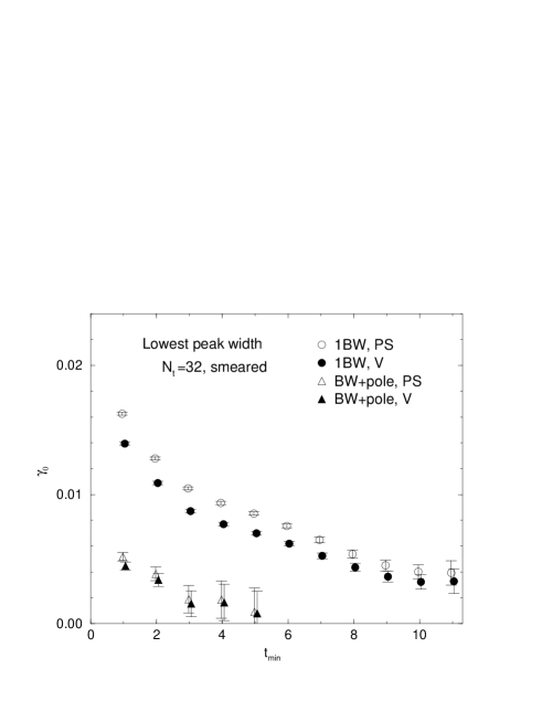
Figure 11: The result of $\chi^{2}$ fit analysis at $N_{t}=32$. The top and bottom panels show the results of the mass and width parameters for the ground state peak, respectively.

According to the result of MEM we can assume that the spectral function of the smeared correlator at this temperature has a peak structure at almost the same mass as at $T=0$ and with small width. Therefore it is expected that the $\chi^{2}$ fits with the three types of fit forms, 2-pole, 1-BW, and BW+pole forms can clarify the low energy structure of the spectral function.

The results are summarized in Fig. 11. The top panel displays the dependence of the mass parameters for the ground state peak on the lower bound of the fit range, $t_{min}$. The upper bound is fixed to $t_{max}=16$. It is apparent that the fit to the 2-pole form exhibits stable results both for the PS and V channels beyond $t_{min}=3$. The result of fit to 1-BW form exhibits no plateau, indicating that this form does not explain the whole structure of the correlators. However, the values seem to approach to the corresponding results of the 2-pole fits. The result of fit to the BW+pole form is consistent with those of 2-pole fit at $t_{min}\leq 2$.

The bottom panel of Fig. 11 shows the result for the width parameter. In the case of the fit to the 1-BW form the value of width gradually decreases with increasing $t_{min}$. This behavior is consistent with a vanishing width. The fit to BW+pole form also indicate that the width is consistent with zero. Therefore, there is no indication of a finite width for the spectral function at this temperature.

All the results of fits to the three forms indicate that the ground state peak is well described by a strong peak with vanishing width, i.e. a pole-like structure, and the associated mass is almost the same as at zero temperature.

VIII Analysis at $T>T_{c}$

VIII.1 Result of MEM analysis

Figure 12: The spectral function at $N_{t}=26$ determined with MEM (smeared correlators).

Figure 13: The results of MEM for the spectral function of the half-smeared correlators at $N_{t}=26$.

In this section, we analyze the correlators at $T\simeq 1.1T_{c}$ ($N_{t}=26$).

The setup of MEM analysis is the same as at $T\simeq 0.9T_{c}$, except for $t_{max}=13$. Figure 12 shows the result. In both the PS and V channels there appear strong peak structures around $\omega\simeq 0.4$. This peak, hereafter called “the ground state peak” for simplicity, appears at almost the same position as at $T\simeq 0.9$ but with larger width. Although, as a common tendency, the peak becomes sharper as the default model parameter $m_{DM}$ increases, the position of the peak is unchanged. It is also verified that the result is essentially the same with less statistics, namely 500 configurations. Therefore it is presumable that the spectral function still has a peak structure at almost the same position as below $T_{c}$.

This result should be compared with the case where the correlators are composed of free quarks, considered in Sec. III.3. In the latter case, as shown in Sec. IV.4, MEM with the present number of degrees of freedom may produce the same feature of the spectral function but with a lower peak position. The above result therefore does not exclude the possibility that the correlators are composed of two weakly interacting quarks with rather large effective mass.

To judge between almost free quarks and genuine bound-state-like structure we analyze the half-smeared correlator. We repeat the same analysis as applied to the smeared correlators for the half-smeared correlators and verify that MEM works up to $t_{max}=12$ on almost the same level as for the smeared ones. As discussed in Sec. IV.4, if the correlator is composed of two almost free quarks the extracted spectral function should exhibit now a wider peak at a higher position. Figure 13 shows the result of MEM analysis for the half-smeared correlators. The analysis is performed in the same manner as for the smeared correlators. Comparing with the result for the smeared correlator, the peak position for the half-smeared one is almost unshifted, while the width of the peak tends to broaden slightly. The latter effect , however, can also be easily explained as an effect of default model uncertainty. This result contradicts therefore the assumption that the peak structure is an artifact of the smearing. Hence the MEM analysis supports a bound-state-like structure at this temperature.

VIII.2 Result of $\chi^{2}$ fit analysis

Figure 14: The result of $\chi^{2}$ fit analysis for the smeared correlators at $N_{t}=26$.

Figure 15: The result of $\chi^{2}$ fit analysis for the half-smeared correlators at $N_{t}=26$.

Figure 16: The spectral functions obtained with $\chi^{2}$ fit analysis at $N_{t}=26$. For the correlators composed of free quarks only the result of BW fit is displayed, while a BW+pole fit is used for the correlators measured in the simulation.

According to the result of MEM, it is reasonable to assume that the spectral function at this temperature also have a peak structure, similarly to the $T<T_{c}$ case. Therefore the three forms for the $\chi^{2}$ fit analysis are still reasonable assumptions to investigate the low energy structures of the correlators.

Figure 14 shows the result of the $\chi^{2}$ fit analysis for the smeared correlators. The top panel shows the $t_{min}$ dependence of the mass parameters. In contrast to the case below $T_{c}$, the masses from 2-pole fit no longer approach those of the other two fit forms but fall monotonously. The masses from 1-BW and BW+pole fits exhibit consistent behaviors, indicating that these fits represent better the correlators. Actually the values of $\chi^{2}/N_{DF}$ are consistently fluctuating around unity at $t_{min}>8$ for 1-BW fit, and in the whole range of $t_{min}$ for BW+pole fit. In the BW+pole fit, the mass parameters for the second peaks take values around 0.9 and 1.0 for PS and V channels, respectively, which is roughly consistent with the result of MEM. The consistency of 1-BW and BW+pole fits also holds for the width parameters, as displayed in the bottom panel of Figure 14. These results indicate therefore that the widths associated with the ground state peaks are finite for both the correlators in PS and V channels.

We now analyze the half-smeared correlators to examine whether this observation of peak structure is an artifact of the smearing. The analysis is performed in the same manner as for the (fully) smeared correlators. The result is displayed in Figure 15. The mass parameters for the half-smeared correlators (top panel) show a similar tendency as for the smeared correlators, although the result of 1-BW and BW+pole fits approach slightly larger values than those of smeared correlators. The shifts of the masses are at most 5% and can be explained with the frequency dependence of the overlap $R(\omega)$ in Eq. (13). A similar tendency is also found for the width parameters in the bottom panel of Fig. 15, which appear even more consistent with those of smeared correlators than the mass parameters. Therefore we find no significant shift of the peak position or broadening of the peak width, such as expected for the case with almost free quarks discussed in Sec. III.3.

Figure 16 illustratively compares these spectral functions extracted with the $\chi^{2}$ fits from four kinds of correlators: the smeared and half-smeared correlators, numerically measured and composed of free quarks. The results of the numerical simulation are of the BW+pole fit with $t_{min}=4$. For the free quark case the results of 1-BW fit with $t_{min}=8$ is displayed. We note that the normalizations of the spectral functions are not significant in the present analysis. In both the PS and V channels the spectral functions for the numerically observed correlators strongly peak near $\omega=0.4$ with small widths. The effect of the smearing seems not significant. In contrast, the spectral functions for the correlators composed of free quarks are strongly dependent on the applied smearing. Both a sizable shift of mass and a broadening of width are observed in this case. It is difficult to exclude completely the possibility that the correlators are composed of almost free quarks with rather large effective mass and nontrivial dispersion relation. However, it is quite suggestive that a nontrivial structure indicating the existence of bound-state-like structure in the low energy region of spectral function subsists at this value of $T$.

Summarizing the results of MEM and $\chi^{2}$ fit analysis we conclude that the charmonium correlators in PS and V channels at $T\simeq 1.1T_{c}$ possess a nontrivial peak structure in the low energy region. As representative values of $m_{0}$ and $\gamma_{0}$, we quote the results of the BW+pole fit analysis with $t_{min}=4$ for the smeared correlators:

$$\mbox{PS}: m_{0}=3.06(2)\mbox{ GeV},\ \ \gamma_{0}=0.12(3)\mbox{ GeV},$$ (40)

$$\mbox{V}: m_{0}=3.13(2)\mbox{ GeV},\ \ \gamma_{0}=0.21(2)\mbox{ GeV}.$$ (41)

The quoted errors in $m_{0}$ and $\gamma_{0}$ are only the statistical ones and do not include the error in $a_{\tau}^{-1}$. As obvious from the discussions in this sections, these results should contain systematic uncertainties of the order of 5% due to the analysis procedures, apart from other uncertainties such as finite lattice artifacts and quenching effects. Compared with the result at $T\simeq 0.9T_{c}$, the widths at $T\simeq 1.1T_{c}$ is sizable, indicating a genuine temperature effect in the deconfined phase. On the other hand, the masses are almost unchanged. This result is contradictory to the absence of bound states argued from the potential model approach MS86 ; Potential_model .

IX Conclusion

The main goals of this paper were (1) to elucidate the technical problems in extraction of the spectral function from lattice data of $t$-correlators, and (2) to investigate the temperature effect on the spectral function near the deconfining phase transition. In the following, we summarize and discuss the results obtained in this paper.

As techniques to extract the information on the spectral function we examined maximum entropy method (MEM) and the standard $\chi^{2}$ fit assuming suitable forms of the spectral function. It is essential to check the reliability of the applied methods to the systems in question. Our condition for reliability at finite temperature is that the methods reproduce the correct form of the spectral function at $T=0$ when the $t$-interval is restricted to the one forced on us at $T>0$. We examined MEM by applying it to the point and smeared correlators. We find that MEM does not meet this requirement for the former, while it does for the latter. This is understandable, since the smearing enhances the low energy part of the spectral function, which is what we are interested in, while a much wide energy region contributes to the point correlators. We note that whether MEM correctly works or not depends primarily on the extension of the physical $t$-region. In particular, for the point correlators a region of $t$ of $O(1\mbox{fm})$ is necessary. For the smeared correlator, this condition is much relaxed. Therefore only the smeared correlators were analyzed at finite temperatures.

Since MEM is ambiguous concerning the quantitative detail of the spectral function, the latter should be also analyzed with other procedures. As such a procedure, the $\chi^{2}$ fit is a reasonable candidate, since MEM already gives a hint for a suitable ansatz for the spectral function. With several assumed forms and examining the fit range dependence of the resultant values for the parameters, this procedure gives us more quantitative information on the properties of spectral function. We emphasize that MEM and $\chi^{2}$ fit analysis as used here are complementary to each other. This two-step approach actually worked for analyses of the correlators at finite temperature, as well as at $T=0$.

Now we discuss the physical implications of our results below and above the critical temperature. We remind that our numerical simulation was performed without dynamical quark effects.

Below the deconfining temperature, at $T\simeq 0.9T_{c}$, the reconstructed spectral function has a strong peak corresponding to the ground state, with almost the same mass as at $T=0$ and narrow width consistent with zero. In contrast to the potential model analysis Has86 , the charmonium mass is not changed up to this temperature. Similar tendencies have been reported in previous lattice QCD calculations for the mesonic channels TARO01 ; Ume01 , while sizable reduction of mass has been observed for glueballs ISM02 . Considering the rather quantitative success of the potential model approach for the charmonium systems at $T=0$ Cornel , it is important to explain this discrepancy.

At $T\simeq 1.1T_{c}$ we observed an indication that the spectral functions still has strong peaks at almost the same positions as $T<T_{c}$, and with widths of about 0.12 and 0.21 GeV for PS and V channels, respectively. This result presumably indicates the existence of quasi-stable bound-state-like structures persistent up to this temperature. The possibility of observing correlators composed of almost free quarks (but of large effective masses) is, however, not completely excluded. Finally, also above $T_{c}$ the observations are not in accord with the expectation from the potential model approach Potential_model . This result implies that the plasma phase has a nontrivial structure at least near the critical temperature.

For a more definite understanding of hadronic correlators at $T>0$ more studies containing dynamical simulations are necessary, as well as calculations in wider range of temperatures. The techniques adopted in this paper should be applicable to these situations. It is also important to repeat the same sort of analysis in the light hadron sectors, for which a nontrivial structure of correlators above $T_{c}$ was also reported TARO01 .

References

- (1) T. Hashimoto, O. Miyamura, K. Hirose and T. Kanki, Phys. Rev. Lett. 57, 2123 (1986).
- (2) T. Matsui and H. Satz, Phys. Lett. B 178, 416 (1986).
- (3) NA50 Collaboration, M. C. Abreu et al., Phys. Lett. B 477, 28 (2000).
- (4) For a review, H. Satz, Nucl. Phys. B (Proc. Suppl.) 94, 204 (2001).
- (5) A.A. Abrikosov, L.P.Gor’kov, and Dzyaloshinskii, Sov. Phys. JETP 36(9), 636 (1959); E.S. Fradkin, Sov. Phys. JETP 36(9), 912 (1959).
- (6) T. Hashimoto, A. Nakamura and I. O. Stamatescu, Nucl. Phys. B400, 267 (1993); Nucl. Phys. B406, 325 (1993).
- (7) QCD-TARO Collaboration, Ph. de Forcrand et al., Phys. Rev. D 63, 054501 (2001).
- (8) T. Umeda, R. Katayama, O. Miyamura and H. Matsufuru, Int. J. Mod. Phys. A 16, 2215 (2001).
- (9) Y. Nakahara, M. Asakawa and T. Hatsuda, Phys. Rev. D 60, 091503 (1999); M. Asakawa, T. Hatsuda and Y. Nakahara, Prog. Part. Nucl. Phys. 46, 459 (2001).
- (10) For pioneering works, QCD-TARO Collaboration, Ph. de Forcrand et al., Nucl. Phys. B (Proc. Suppl.) 63, 460 (1998); E. G. Klepfish, C. E. Creffield, E. R. Pike, ibid., 655 (1998).
- (11) I. Wetzorke and F. Karsch, hep-lat/0008008.
- (12) M. Oevers, C. Davies and J. Shigemitsu, Nucl. Phys. B (Proc. Suppl.) 94, 423 (2001).
- (13) CP-PACS Collaboration, T. Yamazaki et al., Phys. Rev. D 65, 014501 (2002).
- (14) H. R. Fiebig, Phys. Rev. D 65, 094512 (2002); H. R. Fiebig, LHP collaboration, Nucl. Phys. B (Proc. Suppl.) 106, 344 (2002).
- (15) Difficulty in extracting transport coefficients from lattice data has been pointed out in: G. Aarts and J. M. Martinez Resco, JHEP 0204, 053 (2002); hep-lat/0209033.
- (16) F. Karsch, E. Laermann, P. Petreczky, S. Stickan and I. Wetzorke, Phys. Lett. B530, 147 (2002); I. Wetzorke et al., Nucl. Phys. B (Proc. Suppl.) 106, 510 (2002).
- (17) P. Petreczky, F. Karsch, E. Laermann, S. Stickan and I. Wetzorke, Nucl. Phys. B (Proc. Suppl.) 106, 513 (2002).
- (18) S. Datta, F. Karsch, P. Petreczky and I. Wetzorke, hep-lat/0208012.
- (19) M. Asakawa, T. Hatsuda and Y. Nakahara, hep-lat/0208059.
- (20) N. Ishii, H. Suganuma and H. Matsufuru, Phys. Rev. D 66, 014507 (2002); hep-lat/0206020, to appear in Phys. Rev. D.
- (21) K. Nomura, O. Miyamura, T. Umeda and H. Matsufuru, hep-lat/0209139.
- (22) F. Karsch, Nucl. Phys. B205, 285 (1982).
- (23) J. Harada, A. S. Kronfeld, H. Matsufuru, N. Nakajima and T. Onogi, Phys. Rev. D 64, 074501 (2001).
- (24) H. Matsufuru, T. Onogi and T. Umeda, Phys. Rev. D 64, 114503 (2001).
- (25) G. P. Lepage and P. B. Mackenzie, Phys. Rev. D 48, 2250 (1993).
- (26) G.P.Lepage, Nucl. Phys. B (Proc. Suppl.) 26, 45 (1992); P. B. Mackenzie, ibid. 30, 35 (1993); A. S. Kronkeld, ibid. 30, 445 (1993).
- (27) T. R. Klassen, Nucl. Phys. B533, 557 (1998).
- (28) R. Sommer, Nucl. Phys. B411, 839 (1994).
- (29) J. Harada, H. Matsufuru, T. Onogi and A. Sugita, Phys. Rev. D 66, 014509 (2002).
- (30) QCD-TARO Collaboration, S. Choe et al., Nucl. Phys. B (Proc.Suppl.) 106, 361 (2002).
- (31) Particle Data Group Collaboration, D. E. Groom et al., Eur. Phys. J. C 15 (2000) 1.
- (32) F. Karsch, M. T. Mehr and H. Satz, Z. Phys. C 37, 617 (1988).
- (33) E. Eichten, K. Gottfried, T. Kinoshita, K. D. Lane and T. M. Yan, Phys. Rev. D 17, 3090 (1978); 21, 313(E) (1980); 21, 203 (1980).