Novel Approach to Super Yang-Mills Theory on Lattice
- Exact fermionic symmetry and “Ichimatsu” pattern -

Abstract:

We present a lattice theory with an exact fermionic symmetry, which mixes the link and the fermionic variables. The staggered fermionic variables may be reconstructed into a Majorana fermion in the continuum limit. The gauge action has a novel structure. Though it is the ordinary plaquette action, two different couplings are assigned in the “Ichimatsu pattern” or the checkered pattern. In the naive continuum limit, the fermionic symmetry survives as a continuum (or an $O(a^{0})$) symmetry. The transformation of the fermion is proportional to the field strength multiplied by the difference of the two gauge couplings in this limit. This work is an extension of our recently proposed cell model toward the realization of supersymmetric Yang-Mills theory on lattice.

1 Introduction

The importance to formulate the super Yang-Mills theory (SYM) on lattice cannot be overemphasized[1]. Most of previous approaches[2]-[4] to the problem are based on the idea of Curci-Veneziano[5]. According to them, theories do not have any fermionic symmetry at a finite lattice constant and the supersymmetry shows up only in the continuum limit. In the absence of an exact symmetry, one must assume a supersymmetric fixed point and investigate the Ward-Takahashi identity for SUSY[2], [7].

In our previous paper[8], we introduced the lattice gauge model with an exact fermionic symmetry. The model will be called the cell model in the present paper. It has a Grassmann variable on each site and plaquettes distributed in the Ichimatsu pattern or the checkered pattern. Assuming the form of the preSUSY transformation for the fermionic and link variables, we derived the relations among the transformation parameters and coefficients in the action. We showed that the relations may be solved by independent variables. Therefore, we concluded that the cell model has the exact fermionic symmetry for a finite lattice spacing.

In order to realize SYM on lattice, there remain several important questions to be resolved. First of all, we would like to recover the spinor structure in the fermionic sector. Second, the role of the peculiar pattern of plaquette distribution must be clearly explained. Third, we would like to see the relation between the continuum SUSY and the exact fermionic symmetry. In the present paper, we would like to address some of the questions listed above.

The peculiar pattern of the plaquettes showed up in the construction of the cell model[8]. However it was not clear whether this pattern is necessary or not for having the fermionic symmetry. Actually, in the present paper, we will show the presence of other two models with an exact fermionic symmetry. Our new models differ from the cell model only in the gauge sector. In our first new model, we exchange the allowed and discarded plaquettes in the cell model. This complimentary pattern, when realized in three dimension, looks like a set of connected pipes (cf. Fig.2). So the model will be called the pipe model. Repeating the similar procedure to our previous paper[8], we show the presence of the preSUSY in sect. 3. The gauge action of the other model is the weighted sum of those of the cell and pipe models. So we call it the mixed model.

There has been a question of a proper continuum limit posed for the cell model: ie, when we switch off the fermion variables, the plaquettes are completely dissolved. In other words, the perturbative picture is not present in the cell model and we are forced to study it in a nonperturbative way. As for the pipe model, we do not encounter the difficulty described above, even when we remove the fermion variables. However, we can show that the pipe model without fermions does not have an appropriate continuum limit[9]. Therefore it is natural to consider the cell and pipe mixed model to overcome this difficulty.

In defining the mixed model, we assign different coupling constant $\beta_{c}$ or ${\beta_{p}}$ to each set of plaquettes. When we consider the preSUSY transformation in the mixed system, we have twice as many parameters associated with the plaquettes compared to the cell model. So it is not so obvious whether we may keep the fermionic symmetry or not. In the present paper, we answer to this question affirmatively.

We will present a naive continuum limit of the preSUSY transformation for the fermionic variable. There, we observe a very important result. The transformation is proportional to the field strength, a good sign toward the continuum SUSY. It is also proportional to the difference of the two coupling constants $\beta_{c}$ and ${\beta_{p}}$. Therefore, if we are to find the expected SUSY algebra in the continuum limit, it would be present only when the two couplings are different.

In relation to the spinor structure, we show that our staggered fermion action produces the Majorana fermion in the continuum limit. So we may say that our mixed theory is the system of the ordinary gauge (but with two different coupling constants) plus the staggered Majorana fermions. However, the complete realization of spinor structure still remains as an unresolved question. Further discussion on this and related points will be found in the last section.

This paper is organized as follows. In the next section, we introduce the cell, pipe and mixed models and derive the conditions for the preSUSY invariance. The conditions obtained here are solved in sect. 3. In sect. 4 we present a brief summary of our discussion of the Majorana staggered fermion given in appendix C. The naive continuum limit of the fermion transformation is to be studied in sect. 5. There we also explain some properties of our models as proper lattice models. The last section is devoted to a summary and discussion. Four appendices are added. Appendix A is more detailed discussion in support for sect. 3. Appendix B is on the reality properties of various quantities. It is explained how our fermion action is related to continuum Majorana fermions in appendix C. In the last appendix, we show, under some conditions, the uniqueness of the models discussed in this paper.

2 The cell + pipe mixed system and its fermionic symmetry

2.1 The cell and pipe models

In our previous paper, we presented the multi-cell model as connected hypercubes. Contrary to the ordinary lattice theory, not all the possible plaquettes are included in the action. In two dimensional model, the allowed and discarded plaquettes form the checkered or the Ichimatsu pattern. Even in an arbitrary space dimension, the cell model carries the same pattern on any two dimensional surfaces (cf. Figs. 1 and 2).

Figure 1: The Ichimatsu pattern and its relation to the cell and pipe models

Here we show that, using the Ichimatsu pattern, we may construct another model, called the pipe model. It differs from the cell model only in the gauge sector. The gauge action includes the set of plaquettes which are complimentary to the cell model.

In order to explain the new model, we take the three dimensional case shown in Figs. 1 and 2 for convenience. Consider the Ichimatsu patterns given in Fig. 1(a). It is easy to see that the cell model is obtained based on the shaded pattern. Take the shaded pattern on the $x_{1}x_{2}$ plane and put the same pattern on every two dimensional surfaces parallel to it; repeat the same for the $x_{2}x_{3}$ and $x_{3}x_{1}$ planes; then, we obtain the cell model in Fig. 1(b). It is also easy to understand that, doing the same for the unshaded one, we obtain the model shown in Fig. 1(c). The figure looks like a connected pipe-like object (see Fig. 1(c)). So let us call this model the pipe model. By construction, allowed plaquettes for the pipe model form a complimentary set to that of the cell model. In Fig. 2, we show how the cell and pipe models look like.

Starting from Fig. 1(a), we obtained the cell and pipe models. Of course, Fig. 1(a) is not the only way to put the Ichimatsu patterns on the three planes; we could have started from the pattern with shaded and unshaded plaquettes exchanged on the $x_{1}x_{2}$ plane, for example. However, later in sect. 5, we will find that the pattern in Fig. 1(a) is uniquely figured out once we require some properties like the rotational invariance.

Though explained for the three dimensional case, clearly the pipe model can be defined for any dimension. Its plaquettes are arranged in the complimentary pattern to that for the cell model.

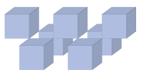
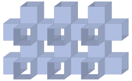
Figure 2: The cell and pipe models.

Figure 3: The shaded plaquettes are for the cell model, $\delta=+1$ and the unshaded ones for the pipe model, $\delta=-1$. Arrows correspond to those in eq. (1) or the most rhs of eq. (2). This figure is for the case of $n_{\mu}=n_{\nu}={\rm even}$.

Now let us find the gauge action for the cell and pipe models. In Fig. 3, we see how the four plaquettes are arranged around the site $n$ on a $\mu-\nu$ plane ($\mu<\nu$). There are always two plaquettes for each model. We introduce the notation $U^{\delta,\epsilon}_{n,\mu\nu}$ to represent each open plaquette. The index $\delta$ is to distinguish the cell ($\delta=+1$) and pipe ($\delta=-1$) models. The other index $\epsilon=\pm 1$ specifies one of the two plaquettes. In concrete, $U^{\delta,\epsilon}_{n,\mu\nu}$ is defined as

$$U^{\delta,\epsilon}_{n,\mu\nu} \equiv U_{n,\epsilon(-)^{n_{\mu}}\mu}U_{n+\epsilon(-)^{n_{\mu}}{\hat{\mu}},\delta\epsilon(-)^{n_{\nu}}\nu}$$ (1)

$$\times~{}U_{n+\delta\epsilon(-)^{n_{\nu}}{\hat{\nu}},\epsilon(-)^{n_{\mu}}\mu}^{\dagger}U_{n,\delta\epsilon(-)^{n_{\nu}}\nu}^{\dagger}.$$

The arrows on Fig. 3 correspond to the directions of the link variables arranged in eq. (1), for the case of $n_{\mu}=n_{\nu}={\rm even}$.

The gauge action may be written as

$$S_{g}^{\delta} = -\frac{\beta_{\delta}}{2}\sum_{n}\sum_{0<\mu<\nu}\sum_{\epsilon=\pm 1}{\rm tr}U^{\delta,\epsilon}_{n,\mu\nu}$$ (2)

$$= -\frac{\beta_{\delta}}{2}\sum_{n}\sum_{0<\mu<\nu}\sum_{\epsilon=\pm 1}{\rm tr}\begin{picture}(88.0,28.0) \put(0.0,0.0){} \put(15.0,-12.0){\vector(1,0){15.0}} \put(40.0,-12.0){\vector(0,1){20.0}} \put(10.0,-7.0){\hbox{}\hbox{ }} \put(15.0,-12.0){\hbox{}\hbox{ }} \put(5.0,-17.0){\makebox(5.0,5.0)[]{\footnotesize$n$}} \put(23.0,-23.0){\makebox(8.0,6.0)[]{\footnotesize$\epsilon(-)^{n_{\mu}}\mu$}} \put(60.0,-2.0){\makebox(8.0,6.0)[]{\footnotesize$\delta\epsilon(-)^{n_{\nu}}\nu$}} \end{picture},$$

where $\beta_{\delta=+1}=\beta_{c}$ and $\beta_{\delta=-1}=\beta_{p}$. Here, for later convenience, we introduced a graphical representation of the open plaquette. By writing $\delta$ in $S^{\delta}_{g}$ explicitly, we mean that the action is for the cell or pipe model. Later we will introduce the cell and pipe mixed model. But here we consider two models separately.

We introduce non-abelian Grassmann variables $\xi\equiv\xi^{a}T^{a}$ to represent a staggered Majorana fermion[10], [11]:

$$S_{f} = \frac{1}{2}\sum_{n}\sum_{\pm\rho}b_{\pm\rho}(n){\rm~{}tr}\,\Bigl{[}\xi_{n}U_{n,\pm\rho}\xi_{n\pm{\hat{\rho}}}U_{n\pm{\hat{\rho}},\mp\rho}\Bigr{]}$$ (3)

$$= \frac{1}{2}\sum_{n}\sum_{\pm\rho}b_{\pm\rho}(n){\rm~{}tr}\,\left[\begin{picture}(60.0,15.0) \put(15.0,-3.0){\@hline} \put(15.0,3.0){\@hline} \put(15.0,3.0){\vector(1,0){20.0}} \put(45.0,-3.0){\vector(-1,0){20.0}} \put(15.0,-3.0){\hbox{}\hbox{ }} \put(15.0,3.0){\hbox{}\hbox{ }} \put(45.0,0.0){\hbox{}\hbox{ }} \put(13.0,8.0){\makebox(5.0,5.0)[]{\footnotesize$n$}} \put(30.0,7.0){\makebox(5.0,5.0)[]{\footnotesize$\pm\rho$}} \end{picture}\right].$$

We use this fermion action for both models. So it does not carry the index $\delta$. In order to have a non-vanishing action, it must hold that $b_{-\rho}(n)=-b_{\rho}(n-{\hat{\rho}})$. Later in sect. 4 we find the expression for $b_{\rho}(n)$ which gives a Majorana fermion in the continuum limit. The expression satisfies this non-vanishing condition. In the figure on the second line of eq. (3), the blobs represent the fermions located at the two sites, while the lines connecting them are link variables. Since the Grassmann variables are present, it is important to keep the order of the variables. So we make the following rule: when we need to recover the equation from a figure, we write down variables following arrows in the figure.

In sect. 4 and appendix C, we will explain how the action (3) is related to the continuum Majorana fermion.

Now we would like to consider a fermionic transformation (the preSUSY transformation) which mixes the link and the fermion variables. We assume the form of the transformation, hoping to realize the ordinary SUSY in a continuum limit. The continuum SUSY transformation of a fermion field is proportional to the field strength. So we take our fermion transformation as follows,

$$\delta\xi_{n}=\sum_{0<\mu<\nu}\sum_{\epsilon=\pm 1}C_{n,\mu\nu}^{\delta,\epsilon}\left(U_{n,\mu\nu}^{\delta,\epsilon}-U_{n,\mu\nu}^{\delta,\epsilon\dagger}\right)$$ (4)

or

$$\delta\left(\begin{picture}(10.0,9.0)\put(5.0,3.0){\hbox{}\hbox{ }} \put(2.0,-8.0){\footnotesize$n$} \end{picture}\right) = \sum_{0<\mu<\nu}\sum_{\epsilon=\pm 1}\left[\begin{picture}(95.0,28.0) \put(0.0,0.0){} \put(33.0,-12.0){\vector(1,0){0.0}} \put(45.0,6.0){\vector(0,1){0.0}} \put(15.0,-6.0){\hbox{}\hbox{ }} \put(15.0,-12.0){\hbox{ }} \put(15.0,-12.0){\makebox(0.0,0.0)[]{$\times$}} \put(28.0,-23.0){\makebox(8.0,6.0)[]{\footnotesize$\epsilon(-)^{n_{\mu}}\mu$}} \put(65.0,-2.0){\makebox(8.0,6.0)[]{\footnotesize$\delta\epsilon(-)^{n_{\nu}}\nu$}} \end{picture}-\begin{picture}(95.0,28.0) \put(0.0,0.0){} \put(70.0,18.0){\vector(1,0){0.0}} \put(50.0,8.0){\vector(0,1){0.0}} \put(50.0,-12.0){\hbox{ }} \put(56.0,-12.0){\hbox{}\hbox{ }} \put(50.0,-12.0){\makebox(0.0,0.0)[]{\bf$\times$}} \put(61.0,23.0){\makebox(8.0,6.0)[]{\footnotesize$\epsilon(-)^{n_{\mu}}\mu$}} \put(22.0,-2.0){\makebox(8.0,6.0)[]{\footnotesize$\delta\epsilon(-)^{n_{\nu}}\nu$}} \end{picture}\right].$$ (5)

The Grassmann transformation parameters are denoted as $C_{n,\mu\nu}^{\delta,\epsilon}$. In the figure they are represented by the crossed circles. In order to distinguish between the cell and pipe models, this $C$-parameter carries the index $\delta$. Later we also use the notation $C_{n,\mu\nu}^{(\epsilon)}$ for $\delta=+1$ and $\bar{C}_{n,\mu\nu}^{(\epsilon)}$ for $\delta=-1$.

The action is to be invariant under the preSUSY transformations of both of the link and fermion variables. So, once eq. (4) is given, the form of the link variable transformation is naturally determined. By introducing Grassmann odd transformation parameters $A$ and $B$, it may be written as

$$\delta U_{n,\mu}=(A\cdot\zeta)_{n,\mu}U_{n,\mu}+U_{n,\mu}(B\cdot\zeta)_{n+{\hat{\mu}},-\mu}$$ (6)

where

$$(A\cdot\zeta)_{n,\mu}\equiv\sum_{\pm\rho}A_{n,\mu}^{\pm\rho}\zeta_{n}^{\pm\rho},~{}~{}~{}~{}~{}(B\cdot\zeta)_{n+{\hat{\mu}},-\mu}\equiv\sum_{\pm\rho}B_{n+{\hat{\mu}},-\mu}^{\pm\rho}\zeta_{n+{\hat{\mu}}}^{\pm\rho},$$ (7)

and

$$\zeta_{n}^{\pm\rho}\equiv U_{n,\pm\rho}\xi_{n\pm{\hat{\rho}}}U_{n,\pm\rho}^{\dagger}.$$ (8)

Eq. (6) implies

$$\delta U_{n,\mu}^{\dagger}=-U_{n,\mu}^{\dagger}\delta U_{n,\mu}U_{n,\mu}^{\dagger}=-(B\cdot\xi)_{n+{\hat{\mu}},-\mu}U_{n,\mu}^{\dagger}-U_{n,\mu}^{\dagger}(A\cdot\xi)_{n,\mu}.$$ (9)

By introducing the notation $U_{n+{\hat{\mu}},-\mu}\equiv U_{n,\mu}^{\dagger}$, we may write eqs. (6) and (9) in a single equation,

$$\delta U_{n,\sigma\mu}=(\alpha\cdot\zeta)_{n,\sigma\mu}U_{n,\sigma\mu}-U_{n,\sigma\mu}({\alpha}\cdot\zeta)_{n+\sigma{\hat{\mu}},-\sigma\mu}$$ (10)

where $\alpha$ are related to $A$ or $B$ in eqs. (6) and (9) as

$$\alpha_{n,\mu}^{\pm\rho}=A_{n,\mu}^{\pm\rho},~{}~{}~{}~{}~{}\alpha_{n,-\mu}^{\pm\rho}=-B_{n,-\mu}^{\pm\rho}.$$

We have three comments. 1) In writing (10) or originally eq. (7), we made a minor change of notation from our previous paper[8]: the minus sign of $-\mu$ of $\alpha_{n+{\hat{\mu}},-\mu}^{\pm\rho}$ indicates the $\alpha$-parameter is located at the end point of the transformed link variable $U_{n,\mu}$. 2) The relation $\delta U^{\dagger}=-U^{\dagger}\delta UU^{\dagger}$ is obtained from the unitarity of the link variable. The result must be the same as $(\delta U)^{\dagger}$. Therefore the quantity $(\alpha\cdot\zeta)$ must be pure imaginary. Then, each term in (10) may be regarded as an infinitesimal form of an unitary transformation acted from the left or the right. This fact is important for the invariance of the path integral measure[8]. 3) Though eq. (10) may look like a gauge transformation, it is not so. In the next section we solve conditions on the parameters for the action invariance. Then we clearly understand that the solution, expressed in terms of independent parameters, does not contain the gauge transformation.

For later convenience, we introduce a graphical representation of eq. (10) as

$$\delta\Bigl{(}\begin{picture}(60.0,30.0)\put(10.0,3.0){ \put(0.0,0.0){\vector(1,0){20.0}} \put(0.0,0.0){\@hline} \put(0.0,0.0){\hbox{}\hbox{ }} \put(30.0,0.0){\hbox{}\hbox{ }} \put(-5.0,-12.0){\footnotesize$n$} \put(15.0,10.0){\footnotesize$\sigma\mu$} \put(20.0,-12.0){\footnotesize$n+\sigma{\hat{\mu}}$} } \end{picture}\Bigr{)}=\sum_{\rho,\sigma^{\prime}}\Big{[}\begin{picture}(60.0,35.0)\put(5.0,3.0){ \put(0.0,10.0){\footnotesize$\sigma^{\prime}\rho$} \put(16.0,-15.0){\footnotesize$n$} \put(30.0,-15.0){\footnotesize$\sigma\mu$} \put(18.0,-3.0){\hbox{ }} \put(21.0,22.0){\hbox{}\hbox{ }} \put(18.0,0.0){\vector(0,1){12.0}} \put(18.0,0.0){\@vline} \put(24.0,22.0){\vector(0,-1){18.0}} \put(24.0,22.0){\@vline} \put(24.0,-3.0){\vector(1,0){18.0}} \put(24.0,-3.0){\@hline} \put(50.0,-3.0){\hbox{}\hbox{ }} } \end{picture}-\begin{picture}(60.0,35.0)\put(5.0,3.0){ \put(12.0,10.0){\footnotesize$\sigma^{\prime}\rho$} \put(2.0,-13.0){\footnotesize$n$} \put(14.0,-15.0){\footnotesize$\sigma\mu$} \put(30.0,-3.0){\hbox{ }} \put(33.0,22.0){\hbox{}\hbox{ }} \put(36.0,-3.0){\hbox{}\hbox{ }} \put(30.0,0.0){\vector(0,1){12.0}} \put(30.0,0.0){\@vline} \put(36.0,22.0){\vector(0,-1){18.0}} \put(36.0,22.0){\@vline} \put(4.0,-3.0){\vector(1,0){18.0}} \put(4.0,-3.0){\@hline} \put(4.0,-3.0){\hbox{}\hbox{ }} } \end{picture}\Bigr{]}.$$ (11)

The circles are for the $\alpha$-parameters.

As is easily realized, the variation of the action under the preSUSY contains terms cubic and linear in the fermion variables. For the action to be invariant, these two set of terms should vanish separately.

The change of the fermion action (3) when link variables are transformed, denoted as $\delta_{U}S_{f}$, consists of fermion cubed terms. A term may be represented by the following figure,

$${\rm~{}tr}\,\left[~{}~{}~{}\begin{picture}(60.0,28.0) \put(0.0,0.0){} \put(14.0,-13.0){\@vline} \put(14.0,-13.0){\vector(0,1){20.0}} \put(20.0,-13.0){\@hline} \put(20.0,-7.0){\vector(1,0){15.0}} \put(14.0,-13.0){\hbox{}\hbox{ }} \put(17.0,17.0){\hbox{}\hbox{ }} \put(44.0,-10.0){\hbox{}\hbox{ }} \put(20.0,-13.0){\hbox{}\hbox{ }} \put(5.0,-20.0){\footnotesize$n$} \put(30.0,0.0){\footnotesize$\sigma\mu$} \put(-5.0,3.0){\footnotesize$\sigma^{\prime}\rho$} \put(0.0,24.0){\footnotesize$n+\sigma^{\prime}{\hat{\rho}}$} \put(28.0,-22.0){\footnotesize$n+\sigma{\hat{\mu}}$} \end{picture}\right].$$ (12)

Here $\sigma$ and $\sigma^{\prime}$ are sign factors. This figure may be generated in two different ways, by the transformation of the link variable $U_{n,\sigma\mu}$ or $U_{n+\sigma^{\prime}\rho,-\sigma^{\prime}\rho}$. Taking care of the sign factor due to the Grassmann nature of the $\alpha$-parameter, we obtain

$$0 = -b_{\sigma\mu}(n)\alpha_{n,\sigma\mu}^{\sigma^{\prime}\rho}+b_{-\sigma^{\prime}\rho}(n+\sigma^{\prime}\rho)\alpha_{n,\sigma^{\prime}\rho}^{\sigma\mu}$$ (13)

$$= -b_{\sigma\mu}(n)\alpha_{n,\sigma\mu}^{\sigma^{\prime}\rho}-b_{\sigma^{\prime}\rho}(n)\alpha_{n,\sigma^{\prime}\rho}^{\sigma\mu}.$$

Note that eq. (13) should hold both for cell and pipe models, independently of $\delta$.

In a similar manner, we may study the cancellation of fermion linear terms, $\delta_{U}S_{g}^{\delta}+\delta_{\xi}S_{f}=0$,

$$0 = \sum_{n,0<\mu<\nu}\sum_{\rho,\epsilon,\sigma}\Biggl{(}-\frac{1}{2}b_{\sigma\rho}(n)\hskip 8.5359pt\begin{picture}(50.0,50.0) \put(0.0,-20.0){ \put(0.0,0.0){} \put(0.0,0.0){} \put(57.0,33.0){\hbox{}\hbox{ }} \put(30.0,36.0){\vector(1,0){16.0}} \put(30.0,27.0){\vector(0,-1){14.0}} \put(30.0,36.0){\hbox{}\hbox{ }} \put(24.0,30.0){\hbox{}\hbox{ }} \put(20.0,36.0){\small$n$} \put(40.0,45.0){\footnotesize$\sigma\rho$} \put(52.0,10.0){\makebox(8.0,6.0)[]{\footnotesize$\epsilon(-)^{n_{\mu}}\mu$}} \put(20.0,-15.0){\makebox(8.0,6.0)[]{\footnotesize$\delta\epsilon(-)^{n_{\nu}}\nu$}} \put(30.0,30.0){\hbox{ }} \put(30.0,30.0){\makebox(0.0,0.0)[]{$\times$}} } \end{picture}$$ (14)

$$-\frac{1}{2}\beta_{\delta}\biggl{(}\hskip 28.45274pt\begin{picture}(50.0,50.0) \put(0.0,0.0){ \put(0.0,0.0){} \put(0.0,0.0){} \put(-3.0,-24.0){\hbox{}\hbox{ }} \put(-6.0,-3.0){\vector(0,-1){14.0}} \put(0.0,0.0){\vector(1,0){16.0}} \put(-6.0,0.0){\hbox{ }} \put(0.0,6.0){\hbox{}\hbox{ }} \put(-10.0,8.0){\footnotesize$n$} \put(-25.0,-20.0){\footnotesize$\sigma\rho$} \put(20.0,-18.0){\makebox(8.0,6.0)[]{\footnotesize$\epsilon(-)^{n_{\mu}}\mu$}} \put(50.0,15.0){\makebox(8.0,6.0)[]{\footnotesize$\delta\epsilon(-)^{n_{\nu}}\nu$}} } \end{picture}\hskip 28.45274pt-\hskip 62.59596pt\begin{picture}(50.0,50.0) \put(0.0,0.0){ \put(0.0,0.0){} \put(0.0,0.0){} \put(-24.0,3.0){\hbox{}\hbox{ }} \put(-3.0,6.0){\vector(-1,0){14.0}} \put(6.0,0.0){\vector(1,0){16.0}} \put(0.0,6.0){\hbox{ }} \put(0.0,0.0){\hbox{}\hbox{ }} \put(6.0,0.0){\hbox{}\hbox{ }} \put(-6.0,-10.0){\footnotesize$n$} \put(-18.0,10.0){\footnotesize$\sigma\rho$} \put(25.0,-15.0){\makebox(8.0,6.0)[]{\footnotesize$\epsilon(-)^{n_{\mu}}\mu$}} \put(50.0,15.0){\makebox(8.0,6.0)[]{\footnotesize$\delta\epsilon(-)^{n_{\nu}}\nu$}} } \end{picture}\hskip 42.67912pt\biggr{)}\Biggr{)}.$$

From eq. (14), we may extract a relation between the transformation parameters. In doing that, remember to follow the arrows in writing down equations from figures. Finally we obtain the relation,

$$\frac{1}{2}b_{\pm\rho}(n)C_{n,\mu\nu}^{\delta,\epsilon}-\frac{\beta_{\delta}}{2}\Bigl{(}\alpha^{\pm\rho}_{n,\epsilon(-)^{n_{\mu}}\mu}-\alpha^{\pm\rho}_{n,\delta\epsilon(-)^{n_{\nu}}\nu}\Bigr{)}=0.$$ (15)

The first term of eq. (15) is from the transformation of $\xi_{n}$ in $S_{f}$. The other two terms are from $\delta_{U}S_{g}^{\delta}$ : the second (third) term is obtained by transforming the link variable $U_{n,\epsilon(-)^{n_{\mu}}\mu}$ ( $U_{n,\delta\epsilon(-)^{n_{\nu}}\nu}$ ). Note that, contrary to eq. (13), eq. (15) is $\delta$-dependent. It is also important to remember that $\pm\rho$ can take any direction, independently $\mu$ and $\nu$.

2.2 Invariance of the cell + pipe mixed system

Up to now, we have studied the cell or pipe model separately. Here we would like to introduce their mixed system and derive the conditions for its preSUSY invariance.

The actions for the cell and pipe models differ in the allowed plaquettes, while the fermion action is independent of $\delta$. As for the preSUSY transformation, the model dependence appears only in eq. (4). These observations are made explicit in the following equations,

$$S=S_{f}+S_{g}^{cell}+S_{g}^{pipe},~{}~{}~{}\delta=\delta_{U}+\delta_{\xi}^{cell}+\delta_{\xi}^{pipe}.$$ (16)

Here the model dependence is written explicitly, rather than indicating it by the sign factor $\delta$. The gauge action consists of two parts, each of them is multiplied by the overall coefficient $\beta_{\delta}$. When two $\beta$ coincide, $\beta_{+1}=\beta_{-1}$ the gauge action is an ordinary plaquette action.

In the transformation of the action

$$\delta S=\delta_{U}S_{f}+\delta_{U}S_{g}^{cell}+\delta_{U}S_{g}^{pipe}+\delta_{\xi}^{cell}S_{f}+\delta_{\xi}^{pipe}S_{f}=0,$$ (17)

three different types of diagrams vanish independently:

$$\delta_{U}S_{f} = 0,$$

$$\delta_{U}S_{g}^{cell} + \delta_{\xi}^{cell}S_{f}=0,$$ (18)

$$\delta_{U}S_{g}^{pipe} + \delta_{\xi}^{pipe}S_{f}=0.$$

Only the first equation contains fermion cubic terms. In the other two equations, different set of plaquettes appear. So it vanishes independently.

Therefore for the invariance of the action, the transformation parameters must satisfy eqs. (13) and (15). In particular, the latter must hold both for $\delta=\pm 1$. These conditions will be solved in the next section.

A comment is in order for the number of transformation parameters in the case of the mixed model. $\delta_{U}$ is the same both for the cell or pipe model. So even for the mixed model, we have the same number of $\alpha$-parameters. The $\delta$ dependence shows up in the fermion transformation. The number of $C$-parameters is doubled for the mixed model, accordingly. Though we solved eqs. (13) and (15) for the cell model, it is not so obvious that we could do the same for the mixed model. This will be discussed in the following section.

3 Solving conditions for the invariance

We obtained the conditions for the action invariance (13) and (15) listed below:

$$b_{\sigma\mu}(n)\alpha_{n,\sigma\mu}^{\sigma^{\prime}\rho} + b_{\sigma^{\prime}\rho}(n)\alpha_{n,\sigma^{\prime}\rho}^{\sigma\mu}=0,$$ (19)

$$b_{\sigma\rho}(n)C_{n,\mu\nu}^{\delta,\epsilon} - {\beta_{\delta}}\Bigl{(}\alpha^{\sigma\rho}_{n,\epsilon(-)^{n_{\mu}}\mu}-\alpha^{\sigma\rho}_{n,\delta\epsilon(-)^{n_{\nu}}\nu}\Bigr{)}=0~{}~{}~{}~{}~{}(\mu<\nu).$$ (20)

The restriction $\mu<\nu$ is due to the definition of $C_{n,\mu\nu}^{\delta,\epsilon}$. Because of this, we need some care in writing equations. In this section, when we have a similar restriction, we write it explicitly as eq. (20) to avoid confusion.

The first equation tells us that $b_{\sigma\mu}(n)\alpha_{n,\sigma\mu}^{\sigma^{\prime}\rho}$ is antisymmetric under the exchange of $\sigma\mu\leftrightarrow\sigma^{\prime}\rho$. From the relation, we may obtain, eg, $\alpha_{n,\sigma\mu}^{\sigma\mu}=0$ or $\alpha_{n,\mu}^{-\mu}-\alpha_{n,-\mu}^{\mu}=0$. By solving eq. (20) for one of the $\alpha$’s, we find that the lower index of the $\alpha$’s can be changed by adding the $C$-parameter.

For the cell model, we solved eqs. (19) and (20) with $\delta=+1$ and find $(2D-1)$ independent parameters at each site[8]. At this moment it is not clear whether we can do the same for the pipe model or the mixed model. For the pipe model, we consider (19) and (20) with $\delta=-1$, while for the mixed model we must solve three conditions, (19) and (20) with $\delta=\pm 1$, corresponding to three equations given in (18). Thus one may consider that we solve different sets of equations for the pipe and mixed models. However we actually can show that effectively the same set of equations are to be solved for both of the mixed and the pipe models. We first explain this observation.

Consider the conditions for pipe model. Eqs. (19) and (20) hold at each site independently. So let us study the conditions at the origin $n=0$ for simplicity. This makes us easy to understand the following discussion without being too much bothered by various sign factors. In appendix A, we will solve the conditions at a generic site. As for $b_{\mu}(n)$, we use the expression to be given in the next section, which produces a Majorana fermion in the continuum limit. At the origin, it takes the values as $b_{\pm\mu}(n=0)=\pm 1$. Thus eqs. (19) and (20) for $\delta=-1$ are written as

$$\sigma\alpha_{~{}~{}\sigma\mu}^{{\sigma}^{\prime}\rho} + {\sigma}^{\prime}\alpha_{~{}~{}{\sigma}^{\prime}\rho}^{\sigma\mu}=0,$$ (21)

$$\bar{C}_{\mu\nu}^{(\epsilon)} - \sigma{\beta_{p}}\Bigl{(}\alpha_{~{}~{}\epsilon\mu}^{\sigma\rho}-\alpha_{~{}-\epsilon\nu}^{\sigma\rho}\Bigr{)}=0~{}~{}~{}~{}(\mu~{}<~{}\nu).$$ (22)

Here we dropped the site index and used the notations $\bar{C}$ and ${\beta_{p}}$ to represent the quantities for $\delta=-1$.

It is easy to derive

$$\bar{C}^{(\epsilon)}_{\lambda\mu}+\bar{C}^{(-\epsilon)}_{\mu\nu}=\sigma{\beta_{p}}\Bigl{(}\alpha_{~{}\epsilon\lambda}^{\sigma\rho}-\alpha_{~{}\epsilon\nu}^{\sigma\rho}\Bigr{)}~{}~{}~{}~{}~{}(\lambda<\mu<\nu).$$ (23)

Though the lhs depends on $\epsilon$, $\mu$, $\nu$ and $\lambda$, the rhs does not depend on the index $\mu$. On top of that, the combination on the rhs of eq. (23) appears in eq. (20) written for $\delta=+1$ and $n=0$,

$$C_{\lambda\nu}^{(\epsilon)}\equiv\sigma{\beta_{c}}\Bigl{(}\alpha_{~{}\epsilon\lambda}^{\sigma\rho}-\alpha_{~{}\epsilon\nu}^{\sigma\rho}\Bigr{)}~{}~{}~{}~{}~{}~{}~{}~{}~{}(\lambda<\nu).$$ (24)

Thus, for the pipe model, we solve three relations (21), (22) and (24); the last relation is regarded as the definitions of $C_{\lambda\nu}^{(\epsilon)}$ and $\beta_{c}$. This is the same set of equations to be solved for the mixed model. Therefore, by solving these three relations, we can consider the pipe and mixed models at once.

Note that $C$ in eq. (24) enjoys the property $C_{\lambda\mu}^{(\epsilon)}+C_{\mu\nu}^{(\epsilon)}-C_{\lambda\nu}^{(\epsilon)}=0~{}~{}~{}~{}~{}(\lambda~{}<~{}\mu~{}<~{}\nu)$ which may be solved as[8]

$$C_{\mu\nu}^{(\epsilon)}=C_{1\nu}^{(\epsilon)}-C_{1\mu}^{(\epsilon)}~{}~{}~{}~{}~{}~{}~{}~{}~{}(1<\mu<\nu).$$ (25)

From eq. (21), we learn that diagonal elements of the $\alpha$-parameter vanish. Using this fact, we may derive the relations between $\alpha$-parameters and $C$-parameters from eqs. (22) and (24),

$$C_{\mu\nu}^{(\epsilon)} = \epsilon{\beta_{c}}\alpha_{~{}\epsilon\mu}^{\epsilon\nu}=-\epsilon{\beta_{c}}\alpha_{~{}\epsilon\nu}^{\epsilon\mu}~{}~{}~{}~{}~{}~{}~{}~{}~{}~{}~{}~{}(\mu<\nu),$$ (26)

$${\bar{C}}_{\mu\nu}^{(\epsilon)} = -\epsilon{\beta_{p}}\alpha_{~{}\epsilon\mu}^{-\epsilon\nu}=-\epsilon{\beta_{p}}\alpha_{~{}-\epsilon\nu}^{\epsilon\mu}~{}~{}~{}~{}~{}~{}~{}~{}~{}(\mu<\nu).$$ (27)

For example, eq. (27) is obtained from eq. (22) by taking $\sigma\rho=-\epsilon\nu$ or $\epsilon\mu$.

As transformation parameters, $C_{\mu\nu}^{(\epsilon)}$ and ${\bar{C}}_{\mu\nu}^{(\epsilon)}$ are associated with the plaquettes for the cell and pipe models, respectively. Through eqs. (26) and (27), we may relate these $\alpha$-parameters to the cell and pipe plaquettes. Note that eq. (22) contains another type of $\alpha$-parameters, $\alpha_{~{}\mu}^{-\mu}=\alpha_{~{}-\mu}^{\mu}$, which do not appear in eqs. (26) and (27). Thus there are three types of $\alpha$-parameters.

Next we show that all the parameters may be written in terms of $\alpha_{1}^{-1}$ and ${C}^{(\epsilon)}_{1\mu}$ (or $\bar{C}^{(\epsilon)}_{1\mu}$).

By using eqs. (25) and (26), the $\alpha$-parameters associated with the cell model may be written as

$$\alpha_{~{}\epsilon\mu}^{\epsilon\nu}=-\alpha_{~{}\epsilon\nu}^{\epsilon\mu}=\frac{\epsilon}{\beta_{c}}\Bigl{(}C^{(\epsilon)}_{1\nu}-C^{(\epsilon)}_{1\mu}\Bigr{)}~{}~{}~{}~{}~{}~{}~{}~{}~{}~{}~{}~{}(\mu<\nu).$$ (28)

Next consider the $\alpha$-parameters associated with the pipe model, $\alpha_{~{}\epsilon\mu}^{-\epsilon\nu}=\alpha_{~{}-\epsilon\nu}^{\epsilon\mu}$. Let us write the relation to shift the lower index of an $\alpha$-parameter, which is obtained from (24) by the replacements, $\lambda\rightarrow 1$ and $\nu\rightarrow\mu$,

$$\alpha_{~{}\epsilon\mu}^{\sigma\rho}=\alpha_{~{}\epsilon 1}^{\sigma\rho}-\frac{\sigma}{\beta_{c}}C^{(\epsilon)}_{1\mu}~{}~{}~{}~{}~{}~{}~{}~{}(\mu>1).$$ (29)

Using eqs. (21) and (29), we find that

$$\alpha_{~{}\epsilon\mu}^{-\epsilon\nu} = \alpha_{~{}\epsilon 1}^{-\epsilon\nu}+\frac{\epsilon}{\beta_{c}}C^{(\epsilon)}_{1\mu}=\alpha^{\epsilon 1}_{~{}-\epsilon\nu}+\frac{\epsilon}{\beta_{c}}C^{(\epsilon)}_{1\mu}=\alpha^{~{}\epsilon 1}_{-\epsilon 1}+\frac{\epsilon}{\beta_{c}}\Bigl{(}C^{(\epsilon)}_{1\mu}-C^{(-\epsilon)}_{1\nu}\Bigr{)}$$ (30)

$$= \alpha_{~{}1}^{-1}+\frac{\epsilon}{\beta_{c}}\Bigl{(}C^{(\epsilon)}_{1\mu}-C^{(-\epsilon)}_{1\nu}\Bigr{)}~{}~{}~{}~{}~{}~{}~{}~{}~{}~{}~{}~{}~{}~{}(1<\mu,\nu,~{}~{}~{}\mu\neq\nu).$$

It would be instructive to explain the above calculation. In the first equality, we shifted the lower index of $\alpha$ by using eq. (29) with $\sigma\rightarrow-\epsilon$ and $\rho\rightarrow\nu$. In the second equality, we exchanged the upper and lower indices by using eqs. (21). We again shifted the (new) lower index in the next expression.

Eq. (30) with (27) gives us the expression of ${\bar{C}}_{\mu\nu}^{(\epsilon)}$ in terms of $\alpha_{1}^{-1}$ and ${C}^{(\epsilon)}_{1\mu}$,

$$\bar{C}_{\mu\nu}^{(\epsilon)}=-\epsilon\beta_{p}\alpha_{~{}1}^{-1}-\frac{\beta_{p}}{\beta_{c}}\Bigl{(}C^{(\epsilon)}_{1\mu}-C^{(-\epsilon)}_{1\nu}\Bigr{)}~{}~{}~{}~{}~{}~{}~{}(\mu<\nu).$$ (31)

We obtain the expression for $\alpha_{-\mu}^{\mu}$ as follows,

$$\alpha_{-\mu}^{\mu} = \alpha_{~{}\epsilon\mu}^{-\epsilon\mu}=\alpha_{~{}~{}\epsilon 1}^{-\epsilon\mu}+\frac{\epsilon}{\beta_{c}}C^{(\epsilon)}_{1\mu}=\alpha_{-\epsilon 1}^{\epsilon 1}-\frac{\epsilon}{\beta_{c}}\Bigl{(}C^{(-\epsilon)}_{1\mu}-C^{(\epsilon)}_{1\mu}\Bigr{)}$$ (32)

$$= \alpha_{~{}-1}^{1}+\frac{1}{\beta_{c}}\Bigl{(}C^{(+)}_{1\mu}-C^{(-)}_{1\mu}\Bigr{)}~{}~{}~{}~{}~{}~{}~{}~{}(\mu>1).$$

Here, in the first equality, use was made of eq. (29) with $\sigma\rightarrow-\epsilon$ and $\rho\rightarrow\mu$.

In summary, we have derived expressions of all the parameters by independent ones, given in eqs. (25), (28), (30), (31) and (32). It is easy to confirm the validity of our results by substituting them back to eqs. (21), and (22) and (24).

Studying relations on the parameters at the origin, we have shown explicitly that all the parameters can be expressed with $\alpha_{~{}~{}1}^{-1}$ and ${C}^{(\epsilon)}_{1\mu}~{}~{}(\mu>1)$. However, it must be obvious that our discussion may be applicable to other sites, that is to be done in appendix A. There, we find 2D-1 independent parameters at each site, $\alpha_{n,1}^{-1}$ and ${C}^{(\epsilon)}_{n,1\mu}~{}~{}(\mu>1)$, the same number as the cell model. Of course, we may choose a different set of independent parameters. In particular, we can take $\bar{C}_{n,1\mu}^{(\epsilon)}$ instead of ${C}_{n,1\mu}^{(\epsilon)}$ (cf. eq. (69)). Leaving the details to appendix A, we quote the expressions of parameters in terms of independent parameters,

$$C_{n,\mu\nu}^{(\epsilon)} = C_{n,1\nu}^{(\epsilon)}-C_{n,1\mu}^{(\epsilon)}=\frac{\beta_{c}}{\beta_{p}}\Bigl{(}\bar{C}_{n,1\nu}^{(-\epsilon)}-\bar{C}_{n,1\mu}^{(-\epsilon)}\Bigr{)}~{}~{}~{}~{}~{}(\mu<\nu),$$ (33)

$$\bar{C}_{n,\mu\nu}^{(\epsilon)} = \frac{\beta_{p}}{\beta_{c}}\Bigl{(}{C}_{n,1\nu}^{(-\epsilon)}-{C}_{n,1\mu}^{(\epsilon)}\Bigr{)}-\epsilon{\beta_{p}}(-)^{n_{1}}\alpha_{n,1}^{-1}$$ (34)

$$= \bar{C}_{n,1\nu}^{(\epsilon)}-\bar{C}_{n,1\mu}^{(-\epsilon)}+\epsilon{\beta_{p}}(-)^{n_{1}}\alpha_{n,1}^{-1}~{}~{}~{}~{}~{}(\mu<\nu).$$

The $\alpha$-parameters may be written as

$$\alpha_{n,\delta\epsilon(-)^{n_{\nu}}\nu}^{\epsilon(-)^{n_{\mu}}\mu}=-\frac{\epsilon(-)^{n_{\mu}}}{\beta_{\delta}}b_{\mu}(n)C_{n,\mu\nu}^{\delta,\epsilon}~{}~{}~{}~{}~{}(\mu<\nu),$$ (35)

$$\alpha_{n,\nu}^{-\nu}=(-)^{n_{\nu}+n_{1}}b_{\nu}(n)\alpha_{n,1}^{-1}+\frac{\epsilon(-)^{n_{\nu}}}{\beta_{c}}b_{\nu}(n)\Bigl{(}C_{n,1\nu}^{(\epsilon)}-C_{n,1\nu}^{(-\epsilon)}\Bigr{)}$$

$$~{}~{}~{}~{}~{}=-(-)^{n_{\nu}+n_{1}}b_{\nu}(n)\alpha_{n,1}^{-1}-\frac{\epsilon(-)^{n_{\nu}}}{\beta_{p}}b_{\nu}(n)\Bigl{(}\bar{C}_{n,1\nu}^{(\epsilon)}-\bar{C}_{n,1\nu}^{(-\epsilon)}\Bigr{)}~{}~{}~{}(\nu>1)$$ (36)

where $\beta_{c}\equiv\beta_{\delta=+1}$.

We conclude that above equations solve the conditions for any model, ie, the cell, the pipe and even the mixed model.

4 The Majorana staggered fermion

Here we consider the reconstruction problem and show that our fermion action in eq. (3) produces a Majorana fermion in a naive continuum limit. We briefly summarize our results and describe the details in appendix C.

We consider the following action,

$$S_{f}=\sum_{n}\eta_{\mu}(n)\xi_{n}\xi_{n+\hat{\mu}}.$$ (37)

The coefficient $b_{\mu}(n)$ in eq. (3) is chosen to be $\eta_{\mu}(n)\equiv(-)^{n_{1}+\cdots n_{\mu-1}}$. As explained in appendix C, this coefficient $\eta_{\mu}(n)$ is naturally obtained when we start from the naively discretized Majorana fermion. The fermion variable $\xi_{n}$ satisfies the reality condition

$$\xi_{n}^{\dagger}=(-)^{|n|}\xi_{n}$$ (38)

so that the action in eq. (37) is real. The condition given in eq. (38) is also discussed in appendix C.

For the reconstruction, we make the identification $\xi_{r}(N)\equiv\xi_{2N+r}$, where $2N$ is the reference coordinate of a hypercube and $r$ is the relative coordinate in the hypercube. In rewriting the action (37), we obtain

$$S_{f} = \frac{1}{2}\sum_{n}\eta_{\mu}(n)\xi_{n}(\xi_{n+\hat{\mu}}-\xi_{n-\hat{\mu}})$$ (39)

$$= \frac{1}{2}\sum_{N,r,\mu>0}\eta_{\mu}(r)\xi_{r}(N){\hat{\partial}}_{\mu}\Bigl{[}\xi_{r+\hat{\mu}}(N)+\xi_{r-\hat{\mu}}(N)\Bigr{]}+\cdots.$$

The higher order terms in the naive continuum limit are denoted by dots. The difference ${\hat{\partial}}_{\mu}$ is defined as

$${\hat{\partial}}_{\mu}\xi_{r^{\prime}}(N) \equiv \frac{1}{2}\Bigl{(}\xi_{r^{\prime}}(N+{\hat{\mu}})-\xi_{r^{\prime}}(N-{\hat{\mu}})\Bigr{)}.$$

Note that, in the reconstruction of the Dirac fermion, we have ${\bar{\xi}}_{r}(N)$ instead of ${\xi}_{r}(N)$ in the second line of eq. (39). In that case, we reach the ordinary action

$$S_{\rm Dirac} = \sum_{N,\mu>0}{\bar{\hat{\psi}}}_{i\alpha}(N)\gamma_{\alpha\beta}{\hat{\partial}}_{\mu}{\hat{\psi}}_{\beta i}(N)+\cdots,$$ (40)

by using the relations,

$$\xi_{r}(N) = \frac{1}{{\cal N}_{0}}{\rm tr}\Bigl{[}V_{r}^{\dagger}{\hat{\psi}}(N)\Bigr{]},$$

$${\bar{\xi}}_{r}(N) = \frac{1}{{\cal N}_{0}}{\rm tr}\Bigl{[}{\bar{\hat{\psi}}}(N)V_{r}\Bigr{]},$$ (41)

and the completeness of $V_{r}\equiv\gamma_{1}^{r_{1}}\gamma_{2}^{r_{2}}\cdots\gamma_{D}^{r_{D}}$. ${{\cal N}_{0}}$ is a normalization coefficient. In eq. (40), the spinor and flavor indices are written as $\alpha$ and $i$, respectively.

In the Majorana staggered fermion case, $\xi_{r}(N)$ must represent two expressions on the rhs of eq. (41). This condition may be realized as the Majorana condition for ${\hat{\psi}}$

$${\hat{\psi}}=C{\bar{\hat{\psi}}}^{T}C^{-1}.$$ (42)

Note that $C^{-1}$ acts on the “flavor” index. From Ref. [12], we find the dimensions to realize the Majorana condition (42): $D=1,2,8~{}~{}({\rm mod}~{}8)$ for Majorana fermions; $D=4,5,6~{}~{}({\rm mod}~{}8)$ for Usp Majorana fermions. The (pseudo-)Majorana fermions in $D=3,7,11$ are not realized this way.

The reality of $\xi_{n}$ is translated into the condition on ${\hat{\psi}}$,

$${\bar{\hat{\psi}}}=\gamma_{D+1}^{\dagger}{\hat{\psi}}^{\dagger}\gamma_{D+1},$$ (43)

where $\gamma_{D+1}$ is a hermitian matrix

$$\gamma_{D+1}\equiv i^{D/2}\gamma_{1}\cdots\gamma_{D}.$$ (44)

Since $\gamma_{D+1}$ can be used as eq. (43) only in the even dimensional spaces, the dimensions listed in the last paragraph must be restricted accordingly. The odd dimensional spaces must be considered separately; the subject will not be discussed in the present paper.

5 On the continuum limit

When we introduced our preSUSY transformation, we first assumed the form of the fermion transformation given in eq. (4). The form was chosen with the expectation that it would produce the continuum SUSY transformation, $\delta\psi\sim\gamma_{\mu\nu}F_{\mu\nu}\epsilon$. Without fully studying the spinor structure, it is not clear whether this is achieved or not. However, as a step toward it, we would like to see its form in the naive continuum limit. This is to be discussed in the next subsection.

The pattern we put the plaquettes may look peculiar. Since we expect an appropriate continuum limit, we confirm, in the second subsection, that our models satisfy reasonable requirements for such a limit. That is, we show that our models have translational and rotational invariances, and satisfy the condition of the reflection positivity[13].

5.1 Continuum limit of the fermion transformation

Here we will show that eq. (4) becomes

$$\delta\xi_{n}\sim\Bigl{(}1-\frac{\beta_{p}}{\beta_{c}}\Bigr{)}2ia^{D/2}g\sum_{0<\mu<\nu}(-)^{n_{\mu}+n_{\nu}}\Bigl{(}C_{n,\mu\nu}^{(+)}+C_{n,\mu\nu}^{(-)}\Bigr{)}F_{n,\mu\nu}$$ (45)

in the naive continuum limit. On the rhs, there follows the terms of the higher order in $a$. So, on the dimensional ground, we would like to keep the rhs of (45), the term with the field strength. If the rhs vanishes, the transformation is higher order in $a$ and vanishes in the continuum limit. Therefore two couplings $\beta_{c}$ and ${\beta_{p}}$ must be different. This implies the importance of the Ichimatsu pattern.

Now we derive eq. (45). A plaquette is related to the field strength as

$$U_{n,\mu\nu}^{\delta,\epsilon}\sim 1+i~{}a^{D/2}gF_{n,\mu\nu}^{\delta,\epsilon}.$$ (46)

Since the direction of the plaquettes are defined as indicated in eq. (2) or Fig. 3, we easily find the relation of the field strength $F_{n,\mu\nu}^{\delta,\epsilon}$ to the ordinary $F_{n,\mu\nu}$ as

$$F_{n,\mu\nu}^{\delta,\epsilon}=\delta(-)^{n_{\mu}+n_{\nu}}F_{n,\mu\nu}.$$ (47)

Using (46) and (47) on the rhs of eq. (4), we find

$$\delta\xi_{n} \sim 2ia^{D/2}g\sum_{\epsilon,\delta}\sum_{0<\mu<\nu}C_{n,\mu\nu}^{\delta,\epsilon}\delta(-)^{n_{\mu}+n_{\nu}}F_{n,\mu\nu}$$

$$= 2ia^{D/2}g\sum_{0<\mu<\nu}(-)^{n_{\mu}+n_{\nu}}\Bigl{(}C_{n,\mu\nu}^{(+)}+C_{n,\mu\nu}^{(-)}-\bar{C}_{n,\mu\nu}^{(+)}-\bar{C}_{n,\mu\nu}^{(-)}\Bigr{)}F_{n,\mu\nu}.$$

Now, note that the relation,

$$\bar{C}_{n,\mu\nu}^{(+)}+\bar{C}_{n,\mu\nu}^{(-)}=\frac{\beta_{p}}{\beta_{c}}\Bigl{(}C_{n,\mu\nu}^{(+)}+C_{n,\mu\nu}^{(-)}\Bigr{)},$$

may be obtained from eq. (34). Thus we have the transformation (45).

Before closing this subsection, it would be worth pointing out that the gauge coupling $g$ is related to $\beta_{c}$ and $\beta_{p}$ as

$$\frac{1}{g^{2}}=\beta_{c}+\beta_{p}.$$ (48)

In the naive continuum limit, the link field may be written as $U_{n,\mu}={\exp}(i~{}a^{\frac{D-2}{2}}~{}g~{}A_{n,\mu})$. Accordingly, the action becomes the sum of terms such as, $a^{D}\beta_{c}g^{2}F^{2}_{\mu\nu}+a^{D}\beta_{p}g^{2}F^{2}_{\mu\nu}$. Thus the relation (48) follows.

5.2 Requirements for a proper continuum theory

Let us see that the cell, pipe and mixed models have some properties so that we may expect an appropriate continuum theory: they are translational and rotational invariant, and they have positive definite transfer matrices. By construction, the three models are translational invariant under the finite translation by $2a$. The Ichimatsu pattern is invariant under the rotation by $\pi/2$ around the center of any plaquette. Our three models have this invariance on any two dimensional plane. That is the rotational invariance of these models.

Osterwalder and Seiler[13] gave a sufficient condition for a model, defined on the Euclidean lattice, to have the positive definite transfer matrix. Let us see that our models satisfy this condition as well. Take any coordinate axis, say $x_{D}$, and regard it as an imaginary time axis. We consider the reflection along this $x_{D}$-axis, denoted as $\theta$,

$$\theta n=\theta(n_{1},n_{2}\cdots,n_{D})=(n_{1},n_{2}\cdots,-n_{D}),$$ (49)

where $(n_{1},n_{2}\cdots,n_{D})$ is the coordinate of a site $n$. In this subsection we assume that $n_{i}$ is a half-integer so that all the sites are reflected under the above action.

Suppose we may define the action of $\theta$ on the fields so that the action $S$ may be written as

$$S=f+\theta f+\sum_{i}(\theta g_{i})g_{i},$$ (50)

for some $f$ and $g$. Then, the transfer matrix is positive definite[13]. So it is important to find out that we can define appropriate transformation of the fields under (49).

As for the link variables, we take the temporal gauge. So it holds that

$$U_{n,D}=\theta U_{n,D}=1.$$ (51)

The reflection acts on the “space”-like link variables as

$$\theta U_{n,k}=U^{\dagger}_{\theta n,k}$$ (52)

where $k=1\sim D-1$. The action of the reflection on the fermion is

$$\theta\xi_{n}=\eta_{D}(n)\xi_{\theta n}.$$ (53)

Following the arguments in [13], the condition (50) on the action may be easily shown.

It may be said that the cell, pipe and the mixed models are natural set of models having three properties: translational and rotational invariances, and the reflection positivity. However it is not trivial that these are the only models having these properties. In appendix D, we consider this point under the restricted situation: we assume the Ichimatsu pattern on every two dimensional surface of the lattice. Under this restriction, we show that our three models are the only models having the three properties.

6 Summary and Discussion

In order to overcome an unnatural feature of the cell model, we introduced the cell-pipe mixed model. The mixed model may be treated perturbatively, contrary to the cell model. Furthermore we showed that the exact fermionic symmetry is present in the mixed model as well. We also have seen that the fermionic sector may be reconstructed as a Majorana fermion in a naive continuum limit. Therefore we may conclude that the staggered Majorana fermion plus the mixed gauge system has the exact fermionic symmetry.

We still have not figured out how the preSUSY could be related to the continuum SUSY. In sect. 5, we looked at the naive continuum limit of the fermion preSUSY transformation. There we observed how the output could contain the field strength. Most importantly, we noticed that the term with the field strength survive in a naive continuum limit only when ${\beta_{p}}/\beta_{c}\neq 1$. This observation in sect. 5 is the only result we have in relation to the continuum SUSY. It is quite interesting that the connection of our preSUSY and the SUSY shows up based on the particular pattern of plaquettes. In other words, we may keep this fermionic symmetry in the continuum limit only when we have the Ichimatsu pattern. For the ordinary lattice ($\beta_{c}=\beta_{p}$), the rhs of eq. (45) vanishes and the transformation will become the higher order in $O(a)$. This observation could be of vital importance.

So, if the fermionic symmetry is really related to the expected SUSY, the continuum limit are to be studied with the cell and pipe mixed model. In particular, we have to approach to the limit keeping the condition ${\beta_{p}}/\beta_{c}\neq 1$. Therefore we would like to see how the theory with ${\beta_{p}}/\beta_{c}\neq 1$ is related to the ordinary one with ${\beta_{p}}/\beta_{c}=1$. In the forthcoming paper[9], we study the $(\beta_{p},\beta_{c})$ phase structure for the pure gauge system.

There are other questions to be resolved. Among others, the recovery of the spinor structure and the doubling problem are crucially important and most difficult. In our formulation, the doubling problem could show up as unbalanced degrees of freedom between the fermion and the gauge field. The situation suggests the higher $N$ SUSY in the continuum theory. Otherwise we have to consider some way to remove unwanted doublers. To understand this point, it would be necessary to reconstruct the spinor structure including that of the transformation parameters.

Acknowledgment
This work is supported in part by the Grants-in-Aid for Scientific Research No. 12640258, 12640259, 13135209, 12640256, 12440060 and 13135205 from the Japan Society for the Promotion of Science.

Appendix A Invariance under infinitesimal transformation

In sect. 3, we solved eqs. (19) and (20) for the site $n=0$. In this appendix, we extend our results there to a generic site $n$.

As in sect. 3 we consider the pipe model and solve the conditions eqs. (19) and (20) for $\delta=-1$. The same logical steps will be taken here as sect. 3.

Rewriting eq. (20) for $\delta=-1$ in the following form

$${\bar{C}_{n,\mu\nu}^{(\epsilon)}}=\frac{\beta_{p}}{b_{\sigma\rho}(n)}\Bigl{(}\alpha^{\sigma\rho}_{n,\epsilon(-)^{n_{\mu}}\mu}-\alpha^{\sigma\rho}_{n,-\epsilon(-)^{n_{\nu}}\nu}\Bigr{)}~{}~{}~{}~{}~{}~{}~{}~{}(\mu<\nu),$$ (54)

we easily find the relation for $\lambda<\mu<\nu$

$${\bar{C}^{(\epsilon)}}_{n,\lambda\mu}+{\bar{C}^{(-\epsilon)}}_{n,\mu\nu}=\frac{\beta_{p}}{b_{\sigma\rho}(n)}\Bigl{(}\alpha^{\sigma\rho}_{n,\epsilon(-)^{n_{\lambda}}\lambda}-\alpha^{\sigma\rho}_{n,\epsilon(-)^{n_{\nu}}\nu}\Bigr{)}\equiv\frac{\beta_{p}}{\beta_{c}}C_{n,\lambda\nu}^{(\epsilon)},$$

Here we have defined the quantity for $\lambda<\nu$

$$C_{n,\lambda\nu}^{(\epsilon)}\equiv\frac{\beta_{c}}{b_{\sigma\rho}(n)}\Bigl{(}\alpha^{\sigma\rho}_{n,\epsilon(-)^{n_{\lambda}}\lambda}-\alpha^{\sigma\rho}_{n,\epsilon(-)^{n_{\nu}}\nu}\Bigr{)}.$$ (55)

There holds the relation, $C^{(\epsilon)}_{n,\lambda\mu}+C^{(\epsilon)}_{n,\mu\nu}-C^{(\epsilon)}_{n,\lambda\nu}=0$ ($\lambda<\mu<\nu$), which may be solved as

$$C^{(\epsilon)}_{n,\mu\nu}=C^{(\epsilon)}_{n,1\nu}-C^{(\epsilon)}_{n,1\mu}~{}~{}~{}~{}~{}~{}~{}~{}(1<\mu<\nu).$$ (56)

This is the first equality of eq. (33).

Eq. (55) is nothing but (20) for $\delta=+1$. Therefore we solve three conditions eqs. (19) and (20) for $\delta=\pm 1$ in the following discussion.

From the symmetry property (19), the diagonal elements of $\alpha$ vanish. Thus we obtain for $\mu<\nu$,

$${\bar{C}_{n,\mu\nu}^{(\epsilon)}} = \frac{\beta_{p}}{b_{\sigma\rho}(n)}\alpha^{\sigma\rho}_{n,\epsilon(-)^{n_{\mu}}\mu}\Bigm{|}_{\sigma\rho=-\epsilon(-)^{n_{\nu}}\nu}=-\frac{\beta_{p}}{b_{\sigma\rho}(n)}\alpha^{\sigma\rho}_{n,-\epsilon(-)^{n_{\nu}}\nu}\Bigm{|}_{\sigma\rho=\epsilon(-)^{n_{\mu}}\mu},$$ (57)

$${{C}_{n,\mu\nu}^{(\epsilon)}} = \frac{\beta_{c}}{b_{\sigma\rho}(n)}\alpha^{\sigma\rho}_{n,\epsilon(-)^{n_{\mu}}\mu}\Bigm{|}_{\sigma\rho=\epsilon(-)^{n_{\nu}}\nu}=-\frac{\beta_{c}}{b_{\sigma\rho}(n)}\alpha^{\sigma\rho}_{n,\epsilon(-)^{n_{\nu}}\nu}\Bigm{|}_{\sigma\rho=\epsilon(-)^{n_{\mu}}\mu},$$ (58)

from eqs. (54) and (55). Using the relation

$$b_{\sigma\nu}(n)=\sigma b_{\nu}(n)~{}~{}~{}~{}~{}~{}(\sigma=\pm 1),$$ (59)

which holds for $b_{\mu}(n)=\eta_{\mu}(n)$, we may further rewrite eqs. (57) and (58). For example, we find

$$\alpha^{-\epsilon(-)^{n_{\nu}}\nu}_{n,\epsilon(-)^{n_{\mu}}\mu}=-\frac{\epsilon}{\beta_{p}}(-)^{n_{\nu}}b_{\nu}(n)\bar{C}_{n,\mu\nu}^{(\epsilon)}~{}~{}~{}~{}~{}(\mu~{}<~{}\nu).$$ (60)

Eqs. (57) and (58) are equivalent to eq. (35).

Let us show that all the parameters may be written in terms of $2D-1$ of them, ie, $\alpha_{n,1}^{-1}$ and ${C}^{(\epsilon)}_{n,1\mu}~{}~{}(\mu>1)$. Later we also show that ${C}^{(\epsilon)}_{n,1\mu}$ can be replaced by $\bar{C}^{(\epsilon)}_{n,1\mu}$.

As explained for the $n=0$ case in sect. 3, there are three kinds of $\alpha$-parameters, $\alpha_{n,\mu}^{-\mu}$, and those associated with the cell and pipe models via the relations in eqs. (58) and (57), respectively.

Using eqs. (56), (58) and (59), the $\alpha$-parameter for the cell model is expressed as

$$\epsilon(-)^{n_{\nu}}\frac{\beta_{c}}{b_{\nu}(n)}\alpha^{\epsilon(-)^{n_{\nu}}\nu}_{n,\epsilon(-)^{n_{\mu}}\mu}=-\epsilon(-)^{n_{\mu}}\frac{\beta_{c}}{b_{\mu}(n)}\alpha^{\epsilon(-)^{n_{\mu}}\mu}_{n,\epsilon(-)^{n_{\nu}}\nu}$$

$$~{}~{}~{}~{}~{}~{}~{}~{}~{}~{}=C^{(\epsilon)}_{n,1\nu}-C^{(\epsilon)}_{n,1\mu}~{}~{}~{}~{}~{}~{}~{}~{}~{}~{}~{}~{}~{}~{}~{}(1<\mu<\nu).$$ (61)

Now consider the $\alpha$-parameter for the pipe model. Rewriting eq. (55), we obtain the relation

$$\frac{1}{b_{\sigma\rho}(n)}\alpha_{n,\epsilon(-)^{n_{\mu}}\mu}^{\sigma\rho}=\frac{1}{b_{\sigma\rho}(n)}\alpha_{n,\epsilon(-)^{n_{1}}1}^{\sigma\rho}-\frac{1}{\beta_{c}}C_{n,1\mu}^{(\epsilon)}$$ (62)

which shifts the lower index. Using eqs. (19) and (62), we find

$$\frac{1}{b_{\sigma\rho}(n)}~{}\alpha^{\sigma\rho}_{n,\epsilon(-)^{n_{\mu}}\mu}\Bigm{|}_{\sigma\rho=-\epsilon(-)^{n_{\nu}}\nu}=-\frac{1}{b_{\sigma\rho}(n)}~{}\alpha^{\sigma\rho}_{n,-\epsilon(-)^{n_{\nu}}\nu}\Bigm{|}_{\sigma\rho=\epsilon(-)^{n_{\mu}}\mu}$$

$$~{}~{}~{}~{}~{}~{}~{}~{}~{}~{}=\frac{1}{b_{\sigma\rho}(n)}~{}\alpha^{\sigma\rho}_{n,\epsilon(-)^{n_{1}}1}\Bigm{|}_{\sigma\rho=-\epsilon(-)^{n_{\nu}}\nu}-\frac{1}{\beta_{c}}C_{n,1\mu}^{(\epsilon)}$$

$$~{}~{}~{}~{}~{}~{}~{}~{}~{}~{}=-\frac{1}{b_{\epsilon(-)^{n_{1}}1}(n)}~{}\alpha^{\epsilon(-)^{n_{1}}1}_{n,-\epsilon(-)^{n_{\nu}}\nu}-\frac{1}{\beta_{c}}C_{n,1\mu}^{(\epsilon)}$$

$$~{}~{}~{}~{}~{}~{}~{}~{}~{}~{}=-\frac{1}{b_{\epsilon(-)^{n_{1}}1}(n)}~{}\alpha^{\epsilon(-)^{n_{1}}1}_{n,-\epsilon(-)^{n_{1}}1}+\frac{1}{\beta_{c}}\Bigl{(}C_{n,1\nu}^{(-\epsilon)}-C_{n,1\mu}^{(\epsilon)}\Bigr{)}$$

$$~{}~{}~{}~{}~{}~{}~{}~{}~{}~{}=-\epsilon(-)^{n_{1}}\alpha^{-1}_{n,1}+\frac{1}{\beta_{c}}\Bigl{(}C_{n,1\nu}^{(-\epsilon)}-C_{n,1\mu}^{(\epsilon)}\Bigr{)}~{}~{}~{}~{}~{}~{}~{}~{}(1<\mu,\nu,~{}~{}~{}\mu\neq\nu).$$ (63)

Let us consider $\alpha_{n,\mu}^{-\mu}$. Again, using eqs. (19) and (62), we obtain

$$-\frac{\epsilon(-)^{n_{\mu}}}{b_{\mu}(n)}\alpha_{n,\mu}^{-\mu} = \frac{1}{b_{\sigma\rho}(n)}\alpha^{\sigma\rho}_{n,\epsilon(-)^{n_{\mu}}\mu}\Bigm{|}_{\sigma\rho=-\epsilon(-)^{n_{\mu}}\mu}$$ (64)

$$= \frac{1}{b_{\sigma\rho}(n)}\alpha^{\sigma\rho}_{n,\epsilon(-)^{n_{1}}1}\Bigm{|}_{\sigma\rho=-\epsilon(-)^{n_{\mu}}\mu}-\frac{1}{\beta_{c}}C_{n,1\mu}^{(\epsilon)}$$

$$= -\frac{1}{b_{\epsilon(-)^{n_{1}}1}(n)}\alpha^{\epsilon(-)^{n_{1}}1}_{n,-\epsilon(-)^{n_{\mu}}\mu}-\frac{1}{\beta_{c}}C_{n,1\mu}^{(\epsilon)}$$

$$= -\frac{1}{b_{\epsilon(-)^{n_{1}}1}(n)}\alpha^{\epsilon(-)^{n_{1}}1}_{n,-\epsilon(-)^{n_{1}}1}+\frac{1}{\beta_{c}}\Bigl{(}C_{n,1\mu}^{(-\epsilon)}-C_{n,1\mu}^{(\epsilon)}\Bigr{)}$$

$$= -\epsilon(-)^{n_{1}}\alpha^{-1}_{n,1}+\frac{1}{\beta_{c}}\Bigl{(}C_{n,1\mu}^{(-\epsilon)}-C_{n,1\mu}^{(\epsilon)}\Bigr{)}.$$

This gives the first line of eq. (36). Note that eqs. (63) and (64) can be summarized by a single equation,

$$\frac{(-)^{n_{\nu}}}{b_{\nu}(n)}~{}\alpha^{-\epsilon(-)^{n_{\nu}}\nu}_{n,\epsilon(-)^{n_{\mu}}\mu}=\frac{(-)^{n_{\mu}}}{b_{\mu}(n)}~{}\alpha^{\epsilon(-)^{n_{\mu}}\mu}_{n,-\epsilon(-)^{n_{\nu}}\nu}=(-)^{n_{1}}\alpha^{-1}_{n,1}+\frac{\epsilon}{\beta_{c}}\Bigl{(}C_{n,1\mu}^{(\epsilon)}-C_{n,1\nu}^{(-\epsilon)}\Bigr{)},$$ (65)

which is valid for $\mu,\nu>1$.

Using eqs. (60) and (65), we find that

$$\frac{1}{\beta_{p}}\bar{C}_{n,\mu\nu}^{(\epsilon)}=-\epsilon(-)^{n_{1}}\alpha_{n,1}^{-1}-\frac{1}{\beta_{c}}\Bigl{(}C_{n,1\mu}^{(\epsilon)}-C_{n,1\nu}^{(-\epsilon)}\Bigr{)},$$ (66)

the first equality of eq. (34). Eq. (66) completes our derivation. All the parameters are written in terms of $\alpha_{n,1}^{-1}$ and ${C}^{(\epsilon)}_{n,1\mu}$ by eqs. (56), (61), (65) and (66).

Finally, we derive the relation between ${C}^{(\epsilon)}_{n,1\mu}$ and $\bar{C}^{(\epsilon)}_{n,1\mu}$. The relation allows us to take $\bar{C}^{(\epsilon)}_{n,1\mu}$ and $\alpha^{-1}_{n,1}$ as independent variables.

We find the relation

$$C_{n,1\nu}^{(-\epsilon)}=\frac{\beta_{c}}{b_{\epsilon(-)^{n_{1}}1}(n)}\Bigl{(}\alpha_{n,1}^{-1}-\alpha_{n,-\epsilon(-)^{n_{\nu}}\nu}^{\epsilon(-)^{n_{1}}1}\Bigr{)}$$ (67)

by making the replacements in eq. (55) as $\lambda\rightarrow 1$, $\epsilon\rightarrow-\epsilon$ and $\sigma\rho\rightarrow\epsilon(-)^{n_{1}}1$. Rewriting (56) for $\mu=1$ with the use of eq. (57), we find that

$$\frac{1}{\beta_{p}}\bar{C}^{(\epsilon)}_{n,1\nu}=\frac{1}{b_{\sigma\rho}(n)}\alpha^{\sigma\rho}_{n,\epsilon(-)^{n_{1}}1}\Bigm{|}_{\sigma\rho=-\epsilon(-)^{n_{\nu}}\nu}=-\frac{1}{b_{\sigma\rho}(n)}\alpha_{n,-\epsilon(-)^{n_{\nu}}\nu}^{\sigma\rho}\Bigm{|}_{\sigma\rho=\epsilon(-)^{n_{1}}1}$$ (68)

Removing $\alpha_{n,-\epsilon(-)^{n_{\nu}}\nu}^{\epsilon(-)^{n_{1}}1}$ from eqs. (67) and (68), we obtain

$$C_{n,1\nu}^{(-\epsilon)}=\epsilon(-)^{n_{1}}\beta_{c}\alpha_{n,1}^{-1}+\frac{\beta_{c}}{\beta_{p}}\bar{C}_{n,1\nu}^{(\epsilon)}.$$ (69)

The expressions of parameters in terms of $\bar{C}^{(\epsilon)}_{n,1\mu}$ and $\alpha^{-1}_{n,1}$ at the end of sect. 3 can be derived by using eq. (69).

Appendix B Reality of various coefficients

Here we study the reality properties of various coefficients. In [8], we noticed that the combination $(\alpha\cdot\zeta)_{n,\sigma\mu}$ must be pure imaginary for the measure invariance. From the definition, the condition may be written as

$$(\alpha\cdot\zeta)_{n,\sigma\mu}^{\dagger}=U_{n,\sigma^{\prime}\rho}\xi_{n+\sigma^{\prime}\rho}^{\dagger}U_{n,\sigma^{\prime}\rho}^{\dagger}(\alpha_{n,\sigma\mu}^{\sigma^{\prime}\rho})^{*}$$ (70)

$$= -(\alpha\cdot\zeta)_{n,\sigma\mu}=-\alpha_{n,\sigma\mu}^{\sigma^{\prime}\rho}U_{n,\sigma^{\prime}\rho}\xi_{n+\sigma^{\prime}\rho}U_{n,\sigma^{\prime}\rho}^{\dagger}.$$

Using eq. (38), we find the relation,

$$(\alpha_{n,\sigma\mu}^{\sigma^{\prime}\rho})^{*}=(-)^{|n|+1}~{}\alpha_{n,\sigma\mu}^{\sigma^{\prime}\rho}.$$ (71)

The consistency of eqs. (4) and (38) implies that

$$(C_{n,\mu\nu}^{\delta,\epsilon})^{*}=(-)^{|n|}C_{n,\mu\nu}^{\delta,\epsilon}.$$ (72)

As for the link variable, it is easy to confirm that the notation $U_{n+{\hat{\mu}},-\mu}\equiv U_{n,\mu}^{\dagger}$ is consistent with eq. (10), when $(\alpha\cdot\zeta)_{n,\sigma\mu}$ is pure imaginary.

Appendix C The Majorana staggered fermion

In the first two subsections we describe how our fermion is related to Majorana fermions naively discretized on lattice. In the last subsection, we discuss the reconstruction problem, ie, how we could obtain the Majorana fermion at the naive continuum limit.

C.1 The Majorana staggered fermion

First take a free Dirac fermion action naively discretized on the lattice,

$$\sum_{n,\mu}\bar{\psi}_{n}\gamma_{\mu}\left(\frac{\psi_{n+\hat{\mu}}-\psi_{n-\hat{\mu}}}{2}\right).$$ (73)

As for the $\gamma_{\mu}$, we follow Kugo’s notation[14][12]. In particular, $\gamma_{\mu}$ are hermitian and thus unitary in the Euclidean space.

We impose the Majorana condition on $\psi$ as

$$\psi_{n}=\psi_{n}^{c}\equiv C{\bar{\psi}}_{n}^{T}.$$ (74)

The charge conjugation matrix $C$ has the properties

$$C^{-1}\gamma_{\mu}C=\eta^{\prime}\gamma_{\mu}^{T},~{}~{}~{}~{}~{}C^{T}=\varepsilon^{\prime}C.$$ (75)

with sign factors $\eta^{\prime}$ and $\varepsilon^{\prime}$. In Ref. [12] one finds the table relating the space dimension to the allowed values for these factors. When the fermion carries the flavor indices, we may impose other Majorana conditions. That possibility is not discussed in this paper.

Following the standard procedure[15], we rewrite the action in terms of the new variables $\omega_{n}$ defined as

$$\psi_{n}\equiv V_{n}\omega_{n}\ ,\ \ \omega_{n}=\left(\begin{array}[]{c}\xi_{n}^{(1)}\\ \xi_{n}^{(2)}\\ \vdots\end{array}\right)$$ (79)

where

$$V_{n}\equiv\gamma_{1}^{n_{1}}\gamma_{2}^{n_{2}}\cdots\gamma_{d}^{n_{d}}.$$ (80)

The fermion action is now expressed as

$$\sum_{n,\mu}\bar{\psi}_{n}\gamma_{\mu}\left(\frac{\psi_{n+\hat{\mu}}-\psi_{n-\hat{\mu}}}{2}\right) = \frac{\varepsilon^{\prime}}{2}\sum_{n,\mu>0}(\eta^{\prime})^{|n|}\eta_{\mu}(n)\Bigl{[}\omega_{n}^{T}C^{-1}(\omega_{n+{\hat{\mu}}}-\omega_{n-{\hat{\mu}}})\Bigr{]}$$ (81)

$$= \frac{1}{2}(\varepsilon^{\prime}+\eta^{\prime})\sum_{n,\mu>0}(\eta^{\prime})^{|n|}\eta_{\mu}(n)~{}\omega_{n}^{T}C^{-1}\omega_{n+{\hat{\mu}}}.$$

In the second equality, the use has been made of the relation

$${\omega_{n}}^{T}C^{-1}\omega_{n+\hat{\mu}}=-{\omega_{n+\hat{\mu}}}^{T}(C^{-1})^{T}\omega_{n} \longrightarrow -{\omega_{n}}^{T}(C^{-1})^{T}\omega_{n-\hat{\mu}}.$$

$$\scriptstyle{n+\hat{\mu}\rightarrow n}$$

From eq. (81), it is easy to see that the lattice Majorana fermion is allowed if

$$\varepsilon^{\prime}\eta^{\prime}=+1.$$ (82)

Following the standard procedure for the staggered Dirac fermion, we would like to reduce the number of degrees of freedom on a site. Suppose we have only one independent component in $\omega_{n}$, ie,

$$\omega_{n}=\xi_{n}u_{0}$$ (83)

with $u_{0}$ as a constant spinor. Then we have

$${\omega_{n}}^{T}C^{-1}\omega_{n+\hat{\mu}}=\xi_{n}\xi_{n+\hat{\mu}}\Bigl{(}{u_{0}}^{T}C^{-1}u_{0}\Bigr{)}~{}~{}\propto~{}~{}\left\{\begin{array}[]{cc}=0&~{}~{}~{}(\varepsilon^{\prime}=-1)\\ \neq 0&~{}~{}~{}(\varepsilon^{\prime}=+1)\end{array}\right.$$ (86)

owing to the property of the charge conjugation matrix. Therefore we may conclude that the expression (83) is allowed only for the case of $\varepsilon^{\prime}=+1$ (and $\eta^{\prime}=+1$). In this case, the action (81) becomes the fermion action (3), up to an irrelevant normalization coefficient,

$$S_{\rm naive}=\Bigl{(}{u_{0}}^{T}C^{-1}u_{0}\Bigr{)}\sum_{n,\mu}\eta_{\mu}(n)\xi_{n}\xi_{n+{\hat{\mu}}}.$$ (87)

We can derive the reality condition on $\xi_{n}$,

$$\xi_{n}^{\dagger}=\frac{(u_{0}^{T}C^{-1}u_{0})}{(u_{0}^{\dagger}\gamma_{D+1}u_{0})}(-\eta^{\prime})^{|n|}\xi_{n},$$ (88)

from the Majorana condition (74) and the definition of ${\bar{\psi}}$

$${\bar{\psi}}\equiv\psi^{\dagger}\gamma_{D+1}.$$ (89)

Though $\eta^{\prime}=1$, we leave eq. (88) as it is to remember where the sign factor comes from.

The matrix $\gamma_{D+1}$, given in eq. (44), is available only for even dimensional space. So the definition (89) of ${\bar{\psi}}$ is valid for that case. The odd dimensional cases require separate consideration, that will not be discussed in this paper.

From the way $\xi_{n}$ and $u_{0}$ appeared in eq. (83), clearly we have the freedom to multiply a phase factor and its inverse to $\xi_{n}$ and $u_{0}$ simultaneously, In particular, we may make positive the coefficient of the action (87) or the numerator of eq. (88). Therefore the fermion action and the reality condition on the fermionic variable can be chosen as

$$S_{\rm naive}=\sum_{n,\mu}\eta_{\mu}(n)\xi_{n}\xi_{n+{\hat{\mu}}},$$ (90)

and

$$\xi_{n}^{\dagger}=(-\eta^{\prime})^{|n|}\xi_{n}.$$ (91)

The denominator of eq. (88), ${(u_{0}^{\dagger}\gamma_{D+1}u_{0})}$, is obviously real. Therefore the coefficient on the rhs of eq. (88) is either $+1$ or $-1$. In writing eqs. (90) and (91), we ignored this possible sign factor.

This is how we reached the fermion action and the reality condition used in this paper.

In the next subsection, we consider the reconstruction problem starting from the action (90). Soon we realize that the reduction from eq. (73) and the reconstruction from eq. (90) give rise different conditions on the sign factors $\varepsilon^{\prime}$ and $\eta^{\prime}$. This is no surprise, since we reduced the number of degrees of freedom as (83) in the middle of the reduction process. In considering the proper continuum limit, the reconstruction problem and its results are far more important than the reduction.

C.2 Reconstruction problem for the free Majorana fermion

In this subsection we reconstruct the (free) Majorana fermion on the lattice with the spacing $2a$. We start from the action (3)

$$S_{f}=\sum_{n,\mu}\eta_{\mu}(n){\rm tr}(\xi_{n}\xi_{n+{\hat{\mu}}})=\frac{1}{2}\sum_{n,\mu>0}\eta_{\mu}(n){\rm tr}(\xi_{n}\xi_{n+{\hat{\mu}}}-\xi_{n}\xi_{n-{\hat{\mu}}}).$$ (92)

The action (92) is real with the reality condition assigned on the fermion $\xi_{n}^{\dagger}=(-)^{|n|}\xi_{n}$ (see appendix B). Note that the coefficient in the fermion action is taken as $b_{\mu}(n)=\eta_{\mu}(n)$.

We understand that the degrees of freedom are distributed in a hypercube attached to the reference point $2N=2\times(N_{1},N_{2},\cdots N_{D})$, where $N_{\mu}$ are the integers. So let us write the site coordinates as

$$n_{\mu}\equiv 2N_{\mu}+r_{\mu}.$$ (93)

Here $r_{\mu}$, being the relative coordinate, takes the values of $0$ or $1$. Since $\eta_{\mu}(n)=\eta_{\mu}(r)$, the fermion action may be rewritten as

$$S_{f}=\frac{1}{2}\sum_{N,r}\sum_{\mu>0}\eta_{\mu}(r){\rm tr}\Bigl{(}\xi_{2N+r}\Bigl{[}\xi_{{2N+r+{\hat{\mu}}}}-\xi_{2N+r-{\hat{\mu}}}\Bigr{]}\Bigr{)}.$$ (94)

Collecting the $2^{D}$-fields in the hypercube with the reference coordinate $2N$, we define

$$\xi_{r}(N)\equiv\xi_{2N+r}.$$ (95)

It is easy to find the following relations

$$\xi_{{2N+r+{\hat{\mu}}}} = \sum_{r^{\prime}}\Bigl{[}\delta_{r+{\hat{\mu}},r^{\prime}}\xi_{r^{\prime}}(N)+\delta_{r-{\hat{\mu}},r^{\prime}}\xi_{r^{\prime}}(N+{\hat{\mu}})\Bigr{]},$$

$$\xi_{{2N+r-{\hat{\mu}}}} = \sum_{r^{\prime}}\Bigl{[}\delta_{r-{\hat{\mu}},r^{\prime}}\xi_{r^{\prime}}(N)+\delta_{r+{\hat{\mu}},r^{\prime}}\xi_{r^{\prime}}(N-{\hat{\mu}})\Bigr{]}.$$ (96)

So we have

$$\xi_{{2N+r+{\hat{\mu}}}}-\xi_{2N+r-{\hat{\mu}}}\equiv\sum_{r^{\prime}}\Bigl{[}\delta_{r+{\hat{\mu}},r^{\prime}}{\hat{\partial}}_{\mu}^{L}\xi_{r^{\prime}}(N)+\delta_{r-{\hat{\mu}},r^{\prime}}{\hat{\partial}}_{\mu}^{R}\xi_{r^{\prime}}(N)\Bigr{]}$$ (97)

where we have introduced derivatives with respect to the lattice spacing $2a$,

$${\hat{\partial}}_{\mu}^{L}\xi_{r^{\prime}}(N)\equiv\xi_{r^{\prime}}(N)-\xi_{r^{\prime}}(N-{\hat{\mu}}),~{}~{}~{}~{}~{}{\hat{\partial}}_{\mu}^{R}\xi_{r^{\prime}}(N)\equiv\xi_{r^{\prime}}(N+{\hat{\mu}})-\xi_{r^{\prime}}(N).$$ (98)

Substituting eq. (97) into eq. (3), we obtain

$$S_{f}=\frac{1}{2}\sum_{N,r,r^{\prime}}\sum_{\mu>0}\Bigl{[}\xi_{r}(N)\Bigl{(}\Gamma_{rr^{\prime}}^{\mu}{\hat{\partial}}_{\mu}+\frac{1}{2}\Gamma_{rr^{\prime}}^{5\mu}{\hat{\square}}_{\mu}\Bigr{)}\xi_{r^{\prime}}(N)\Bigr{]}$$ (99)

where

$$\Gamma_{rr^{\prime}}^{\mu}\equiv(\delta_{r+{\hat{\mu}},r^{\prime}}+\delta_{r-{\hat{\mu}},r^{\prime}})\eta_{\mu}(r),~{}~{}~{}\Gamma_{rr^{\prime}}^{5\mu}\equiv(\delta_{r-{\hat{\mu}},r^{\prime}}-\delta_{r+{\hat{\mu}},r^{\prime}})\eta_{\mu}(r),$$

$$~{}~{}~{}~{}~{}~{}~{}{\hat{\partial}}_{\mu}\xi_{r^{\prime}}(N)\equiv\frac{1}{2}\Bigl{(}\xi_{r^{\prime}}(N+{\hat{\mu}})-\xi_{r^{\prime}}(N-{\hat{\mu}})\Bigr{)},$$

$$~{}~{}~{}~{}~{}~{}~{}{\hat{\square}}_{\mu}\xi_{r^{\prime}}(N)\equiv\xi_{r^{\prime}}(N+{\hat{\mu}})+\xi_{r^{\prime}}(N-{\hat{\mu}})-2\xi_{r^{\prime}}(N).$$ (100)

Obviously only the first term survives in the naive continuum limit. Therefore we consider the first term given in eq. (39)

$$S_{f}=\frac{1}{2}\sum_{N,\mu>0,r}\eta_{\mu}(r)\xi_{r}(N){\hat{\partial}}_{\mu}\Bigl{[}\xi_{r+\hat{\mu}}(N)+\xi_{r-\hat{\mu}}(N)\Bigr{]}+\cdots.$$ (101)

We would like to further rewrite the above action in terms of the reconstructed fermion

$${\hat{\psi}}_{\alpha i}(N) \equiv {\cal N}_{0}\sum_{r}(V_{r})_{\alpha i}\xi_{r}(N),$$ (102)

The coefficient ${\cal N}_{0}$ is a normalization constant to be fixed appropriately. Note that $V_{r}$ has the properties

$$\sum_{r}(V_{r}^{\dagger})_{i\alpha}(V_{r})_{\beta j} =2^{\frac{D}{2}} \delta_{\alpha\beta}\delta_{ij},~{}~{}~{}~{}~{}V_{r}^{\dagger}=d_{r}V_{r}$$

$${\rm tr}(V_{r}^{\dagger}V_{r^{\prime}}) = \delta_{rr^{\prime}}2^{\frac{D}{2}},~{}~{}~{}~{}~{}V_{r\pm{\hat{\mu}}}=\eta_{\mu}(r)\gamma_{\mu}V_{r},$$ (103)

where $d_{r}=(-)^{|r|(|r|-1)/2}$ is a sign factor. Reversing the expression (102), we have

$$\xi_{r}(N)=\frac{1}{\cal N}_{0}{\rm tr}\Bigl{[}V_{r}^{\dagger}{\hat{\psi}}(N)\Bigr{]}.$$ (104)

We would like to write the action (99) in terms of ${\hat{\psi}}$. For that purpose, it is useful to remember how it goes for the Dirac fermion. In that case we have ${\bar{\xi}}_{r}$ and ${\xi}_{r}$ which are related to the reconstructed fermions as (41). Using the relation,

$$\sum_{r}\eta_{\mu}(r){\bar{\xi}}_{r}(N){\hat{\partial}}_{\mu}\xi_{r\pm\hat{\mu}}(N) = ({\cal N}_{0})^{-2}\sum_{r}\eta_{\mu}(r){\rm tr}\Bigl{[}{\bar{\hat{\psi}}}(N)V_{r}\Bigr{]}~{}{\hat{\partial}}_{\mu}{\rm tr}\Bigl{[}V_{r\pm\hat{\mu}}^{\dagger}{\hat{\psi}}(N)\Bigr{]}$$ (105)

$$= ({\cal N}_{0})^{-2}2^{D/2}{\bar{\hat{\psi}}}(N)_{i\alpha}(\gamma_{\mu})_{\alpha\beta}{\hat{\partial}_{\mu}}{\hat{\psi}}(N)_{\beta i},$$

the action $S_{\rm Dirac}$ of the (Dirac) staggered fermion can be obtained as

$$S_{\rm Dirac}=\sum_{N,\mu}{\rm tr}\Bigl{[}{\bar{\hat{\psi}}}(N)(\gamma_{\mu}){\hat{\partial}_{\mu}}{\hat{\psi}}(N)\Bigr{]}+\cdots.$$ (106)

Here the normalization constant is chosen as ${\cal N}_{0}=2^{D/4}$.

If we expect to have the relation similar to eq. (105) for the Majorana staggered fermion, $\xi_{r}(N)$ must be related to both ${\hat{\psi}}(N)$ and ${\bar{\hat{\psi}}}(N)$ as

$$\xi_{r}(N)=\frac{1}{{\cal N}_{0}}{\rm tr}\Bigl{[}V_{r}^{\dagger}{\hat{\psi}}(N)\Bigr{]}=\frac{1}{{\cal N}_{0}}{\rm tr}\Bigl{[}{\bar{\hat{\psi}}}(N)V_{r}\Bigr{]}.$$ (107)

For the second equality to hold, we find the Majorana condition on ${\hat{\psi}}$ with $\eta^{\prime}=1$

$${\hat{\psi}}=C{\bar{\hat{\psi}}}^{T}C^{-1}.$$ (108)

The restriction $\eta^{\prime}=1$ may be easily read off from the following relation,

$${\rm tr}\Bigl{[}{\hat{\psi}}V_{r}^{\dagger}\Bigr{]}={\rm tr}\Bigl{[}{\bar{\hat{\psi}}}^{T}C^{-1}\gamma_{D}^{r_{D}}\cdots\gamma_{1}^{r_{1}}C\Bigr{]}={\rm tr}\Bigl{[}{\bar{\hat{\psi}}}^{T}(\eta^{\prime})^{|r|}V_{r}^{T}\Bigr{]}=(\eta^{\prime})^{|r|}{\rm tr}\Bigl{[}{\bar{\hat{\psi}}}V_{r}\Bigr{]}.$$

Eq. (107) and the reality condition on $\xi_{n}$, ie, $\xi_{n}^{\dagger}=(-)^{|n|}\xi_{n}$, imply the relation

$${\bar{\hat{\psi}}}=\gamma_{D+1}^{\dagger}{\hat{\psi}}^{\dagger}\gamma_{D+1},$$ (109)

where $\gamma_{D+1}$ is a hermitian matrix defined in eq. (44). Remember that, for a Euclidean theory, ${\bar{\psi}}\equiv\psi^{\dagger}\gamma_{D+1}$ is the appropriate relation to keep the reality of the action ${\bar{\psi}}(\gamma_{\mu}\partial_{\mu}+m)\psi$. Eq. (109) is a multi-flavored extension of this relation. The matrix $\gamma_{D+1}$ is defined only for even dimensional spaces and we have to consider the odd dimension separately. That is, however, beyond the scope of the present paper.

In Ref.[12], we find the list of Majorana fermions realized by the condition given in eq. (108), as already presented in the sect. 3.

Appendix D Uniqueness of the models

Figure 4: This figure shows how the face $F_{0}$ is related to other faces by four conditions listed in the text.

Here we find out how we can classify the plaquettes in the entire space so that the following four conditions are satisfied: 1) Ichimatsu pattern on any two dimensional surface ; 2) invariance under mod 2 translations; 3) symmetry under ${\pi}/2$ rotations; 4) the reflection positivity. The cell, the pipe and the mixed models are uniquely selected out by the first three conditions; the models have the reflection positivity to allow an appropriate continuum limit, as already discussed in sect. 5.2.

From the condition 1), we are to classify plaquettes into shaded and unshaded sets on every two dimensional surface. In the following, we show that the assignment is uniquely determined by two other conditions. Based on this pattern, we construct the cell, pipe and mixed models. Collecting shaded (unshaded) plaquettes, we obtain the cell (pipe) model. For the mixed model, we give the coefficients $\beta_{c}$ ($\beta_{p}$) to shaded (unshaded) plaquettes. In this sense, the cell, pipe and mixed models are uniquely selected out by the conditions.

The three dimensional case suffices to illustrate our consideration. Take a two dimensional plane and choose the coordinate system so that the plane is the $x_{1}x_{2}$-plane with $x_{D}\equiv x_{3}=0$. On this plane, we take the plaquette closest to the origin in the first quadrant and make it shaded: the plaquette is $F_{0}$ in Fig. 4. Remember that this choice completely determines the Ichimatsu pattern on the plane.

Next we find out how we may realize rotations consistently with the Ichimatsu pattern. Take again the $x_{1}x_{2}$-plane in the last paragraph and consider the $\pi/2$ rotation of this plane which does not affect the Ichimatsu pattern on the plane. Clearly the center of the rotation must be located at the center of a plaquette. Its rotational axis passes through the center of a hypercube, eg, $Q\equiv(1/2,~{}1/2,~{}1/2)$ shown in Fig. 4. Consider two other axes through the same point $Q$ and parallel to $x_{1}$ and $x_{2}$. We are to arrange the pattern in the entire space so that the $\pi/2$ rotations around these axes do not change the pattern.

Although the reflection is not necessary for the present discussion, it is appropriate to mention how the reflection plane should be chosen. The reflection must be consistent with the Ichimatsu patterns in the entire space. There are two types of planes, perpendicular to the $x_{3}$-axis, which respect the lattice structure. One is the $x_{1}x_{2}$-plane and the other is the plane that contains the point $Q$. Obviously the reflection with respect to the former does change the Ichimatsu pattern on the $x_{1}x_{3}$-plane. Therefore the reflection plane must contain the center of a hypercube.

In Fig. 4, the face $F_{0}$ is a shaded plaquette. Using twice the $\pi/2$ rotation around the $x_{1}$ axis, we find that $F_{1}$ must also be shaded. From the invariance under the translation by mod 2, $F_{2}$ is also shaded. These results completely determine the Ichimatsu patterns on planes parallel to the $x_{1}x_{2}$-plane. By the $\pi/2$ rotation around the $x_{1}$ axis, the plaquettes $F_{0}$, $F_{1}$ and $F_{2}$ are brought to those with primes, and the Ichimatsu patterns parallel to the $x_{1}x_{3}$-plane are determined. Obviously, rotations around another axis give the unique and complete classification of all the plaquettes into the shaded and unshaded set. This proves our claim for the three dimensional case. It must be obvious that the proof may be easily extended to any dimension.

References

• [1] For a latest review on the subject, see A. Feo, hep-lat/0210015.
• [2] DESY-Muenster collaboration, I. Campos, A. Feo, R. Kirchner, S. Luckmann, I. Montvay, G. Münster, K. Spanderen, J. Westphalen, Eur. Phys. J. C11 (1999) 507; F. Farchioni, A. Feo, T. Galla, C. Gebert, R. Kirchner, I. Montvay, G. Münster, A. Vladikas, Nucl. Phys. Proc. Suppl. 94 (2001) 787; F. Farchioni, A. Feo, T. Galla, C. Gebert, R. Kirchner, I. Montvay, G. Munster, A. Vladikas, Nucl. Phys. Proc. Suppl. 106 (2002) 938; DESY-Munster-Roma Collaboration (F. Farchioni et al.) Eur. Phys. J. C23 (2002) 719.
• [3] D. B. Kaplan and M. Schmaltz, Chin. J. Phys. 38 (2000) 543.
• [4] G. T.  Fleming, J.  B.  Kogut, P. M.  Vranas, Phys.  Rev. D64 (2001) 034510.
• [5] G. Curci and G. Veneziano, Nucl. Phys. B292 (1987) 555.
• [6] D. B. Kaplan, E. Katz, M. Unsal, hep-lat/0206019, hep-lat/0208046.
• [7] Y. Taniguchi, Phys. Rev. D63 (2001) 014502; Chin. J. Phys. 38 (2000) 655; F. Farchioni, A. Feo, T. Galla, C. Gebert, R. Kirchner, I. Montvay, G. Muenster, R. Peetz and A. Vladikas, Nucl. Phys. Proc. Suppl. 106 (2002) 941.
• [8] K. Itoh, M. Kato, H. Sawanaka, H. So and N. Ukita, Prog. Theor. Phys. 108 (2002) 363 and hep-lat/0209034.
• [9] K. Itoh, M. Kato, H. Sawanaka, M. Murata and H. So, hep-lat/0209030 and in preparation.
• [10] L. Susskind, Phys. Rev. D16 (1977) 3031.
• [11] H. Aratyn, M.  Goto and A. H. Zimerman, Nuovo Cimento A 84 (1984) 255; Nuovo Cimento A 88 (1985) 225; H. Aratyn, P. F. Bessa and A.  H.  Zimerman, Z. Phys. C27 (1985) 535; H. Aratyn, and A. H. Zimerman, J. Phys. A: Math. Gen. 18 (1985) L487.
• [12] T. Kugo and P. K. Townsend, Nucl. Phys. B221 (1983) 357-380.
• [13] K. Osterwalder and E. Seiler, Ann. of Phys. 110 (1978) 440-471.
• [14] T. Kugo, private communication.
• [15] H. J. Rothe, Lattice Gauge Theories: An Introduction (World Scientific) 1997.