Perturbative Wilson loops with massive sea quarks on the lattice

Abstract

We present ${\mathcal{O}}(g^{4})$ calculations of both planar and non-planar Wilson loops for various actions in the presence of sea quarks. In particular, the plaquette, the static potential and the static self energy are calculated to this order for massive Wilson, Sheikholeslami-Wohlert and Kogut-Susskind fermions, including the mass and $n_{f}$ dependence. The results can be used to obtain $\alpha_{\overline{MS}}$ and $\overline{m_{b}}(\overline{m_{b}})$ from lattice simulations. We compare our perturbative calculations to simulation data of the static potential and report excellent qualitative agreement with boosted perturbation theory predictions for distances $r<1\,\mbox{GeV}^{-1}$. We are also able to resolve differences in the running of the coupling between $n_{f}=2$ and $n_{f}=0$ static potentials. We compute perturbative estimates of the “$\beta$-shifts” of QCD with sea quarks, relative to the quenched theory, which we find to agree within 10 % with non-perturbative simulations. This is done by matching the respective static potentials at large distances. The prospects of determining the QCD running coupling from low energy hadron phenomenology in the near future are assessed. We obtain the result $\Lambda^{(2)}_{\overline{MS}}r_{0}=0.69(15)$ for the two flavour QCD $\Lambda$-parameter from presently available lattice data where $r_{0}^{-1}\approx 400$ MeV and estimate $\alpha_{\overline{MS}}^{(5)}(m_{Z})=0.1133(59)$.

I Introduction

The calculation of Wilson loops in lattice perturbation theory is useful in a number of ways. An important application is the prediction of a strong coupling constant $\alpha_{\overline{MS}}^{(5)}(m_{Z})$ from low energy hadronic phenomenology by means of non-perturbative lattice simulations El-Khadra:1992vn ; davi1 ; davi2 ; Spitz:1999tu ; Booth:2001qp ; davi3 . Perturbative calculations of Wilson loops are also employed in the context of mean field improvement programmes of the lattice action and operators Parisi:1980pe ; lepage .

In the limit of infinite Euclidean time separation, $T\rightarrow\infty$, Wilson loops give access to the perturbative lattice potential. Our results improve the understanding of the violations of rotational symmetry at short distances of this quantity, as well as of the short distance effects of including various flavours of sea quarks. Furthermore, in the limit of large distances, $R\rightarrow\infty$, the self-energy of static sources can be obtained from the potential, enabling the calculation of $\overline{m_{b}}(\overline{m_{b}})$ from non-perturbative simulations of heavy-light mesons in the static limit Martinelli:1999vt .

Perturbative computations of Wilson loops on the lattice now reach back as far as two decades. For this reason, much of the groundwork for the calculation covered in this article is well known, and has been reproduced by us. In addition to improving the precision of many previously existing results and presenting them in a more comprehensive way, we extend the calculations by incorporating the actions, sea quark masses and observables that are relevant for present day lattice simulations. We also perform the first calculation of non-planar Wilson loops. Because of the degree of replication we present a brief survey of the existing literature here.

In 1981 Müller and Rühl MullerRuhl performed a highly rigorous calculation of the ${\mathcal{O}}(g^{4})$ contribution to the Wilson loop for pure $U(1)$ and $SU(2)$ gauge theories and presented their result in terms of lattice integrals. In particular, they obtained a closed form for the $T\rightarrow\infty$ limit and hence the static potential. The plaquette in $SU(N)$ pure gauge theory was first calculated to this order by Di Giacomo and Rossi DiGiacomo:1981wt , again in 1981. In the same year Hattori and Kawai Hattori:1981ac estimated ${\mathcal{O}}(g^{4})$ contributions to larger Wilson loops, by modelling some of the relevant lattice contributions by their continuum counterparts. Rigorous results to this order were subsequently independently obtained by three groups of authors: Weisz, Wohlert and Wetzel Weisz:1984bn , Curci, Paffuti and Tripiccione Curci:1984wh and Heller and Karsch Heller:1985hx . The first reference is the most general and also applies to Symanzik-improved pure Yang-Mills actions. However, numerical results on Wilson loops are only available for the Wilson action. The ${\mathcal{O}}(g^{4})$ fermionic contribution to the plaquette was obtained by Hamber and Wu Hamber:1983ft for Wilson quarks and for Kogut-Susskind (KS) quarks by Heller and Karsch Heller:1985eq . More recently, Panagopoulos et al. calculated the ${\mathcal{O}}(g^{6})$ $SU(N)$ gluonic contribution Alles:1994dn as well as the ${\mathcal{O}}(g^{4})$ and ${\mathcal{O}}(g^{6})$ corrections Alles:1998is in presence of massive Wilson fermions. The only numerical calculation to-date of small Wilson loops for Symanzik improved gluonic actions was performed by Iso and Sakai Iso:1987dj .

More recently, the Heller and Karsch calculations Heller:1985hx have been extended by Martinelli and Sachrajda Martinelli:1999vt in a manner similar to that of Müller and Rühl MullerRuhl : the $R,T\rightarrow\infty$ limit of the perimeter term of Wilson loops has been taken to obtain the static self energy for $SU(3)$ gauge theory, with the addition of massless Wilson and Sheikholeslami-Wohlert (SW) sea quarks.

The structure of this paper is as follows. In Sec. II we describe the procedure used to calculate Wilson loops in perturbation theory and present the perturbative expansions of small Wilson loops, both planar and non-planar, to ${\mathcal{O}}(g^{4})$ using a variety of actions. Although partially addressed by previous authors Weisz:1984bn ; Curci:1984wh ; Heller:1985hx ; Altevogt:1995cj the static potential has not been well treated in literature, which we attempt to rectify in Sec. III, where we also obtain the static source self energy from the asymptotic $R\rightarrow\infty$ potential. This sets the stage for Sec. IV where these perturbative results are confronted with state-of-the-art lattice data from simulations with Wilson, SW and KS fermions: we determine the “$\beta$-shift” and the running coupling $\alpha_{\overline{MS}}$, before comparing perturbative and non-perturbative potentials at short distances. In Sec. V we conclude and summarize. Our article is augmented by two Appendices on the relations between different lattice and continuum renormalization schemes and on the perturbative $\beta$-shift.

II Wilson loops in lattice perturbation theory

In this section we explain our method and notations, before displaying results on small Wilson loops with massive fermions to ${\mathcal{O}}(g^{4})$. We also include some findings that apply to the Iwasaki and Symanzik-Weisz gauge actions.

II.1 The Method

We consider $SU(N)$ lattice gauge theory on an infinite four dimensional isotropic hyper-cubic lattice with lattice spacing $a$. An oriented closed curve ${\mathcal{C}}$ of length $na$ touches a sequence of sites, $\{x_{i}:x_{i}/a\in{\mathbb{Z}}^{4}\}$ such that $x_{i+1}-x_{i}\in\{\pm a\hat{\mu}:\mu=1,\ldots,4\}$, $x_{n+1}=x_{1}$. The Wilson loop $W({\mathcal{C}})$ around such a curve is the expectation value of the path ordered product of gauge links,

$$W({\mathcal{C}})=\frac{1}{N}\left\langle\mbox{tr}\,\left[\prod_{x_{i}\in{\mathcal{C}}}U_{x_{i},\mu_{i}}\right]\right\rangle,$$ (1)

where $\mu_{i}\in\{\pm 1,\cdots,\pm 4\}$ denotes the direction indicated by $x_{i+1}-x_{i}$ and $U_{x,-\mu}=U^{\dagger}_{x-\hat{\mu},\mu}$.

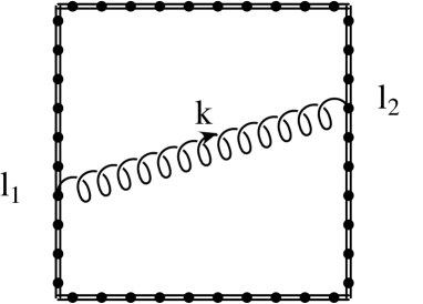
Figure 1: Tree-level [${\mathcal{O}}(g^{2})$] contribution to the Wilson loop. The coordinate space propagator is convoluted around the possible source and sink links of the loop. This is done by constructing the corresponding sum of phase factors in momentum space and Fourier transforming.

We write $W({\mathbf{R}},T)$ for a “rectangular” Wilson loop where the curve ${\mathcal{C}}$ contains two opposite lines with an extent of $T$ lattice units pointing into the time ($\hat{4}$) direction, that are separated by a spatial distance ${\mathbf{R}}a$. The smallest such Wilson loop is an $a\times a$ square, the plaquette $\Box=W(1,1)$ which, appropriately normalized, is the expectation value of the Wilson gauge action,

$$S=-\beta\sum_{x,\mu>\nu}\frac{1}{N}\mbox{Re}\,\mbox{tr}\,U_{x,\mu\nu},$$ (2)

where $\beta=2N/g^{2}$ and $U_{x,\mu\nu}=U_{x,\mu}U_{x+a\hat{\mu},\nu}U^{\dagger}_{x+a\hat{\nu},\mu}U^{\dagger}_{x,\nu}$. Unless stated otherwise this is the gauge action which we combine either with the Wilson, SW or the KS fermionic actions.

Writing $U_{l}=e^{igaA_{l}}$, where $l=(x,\mu)$ denotes the link connecting $x$ with $x+a\hat{\mu}$ and $A_{l}$ is a short hand notation for $A_{\mu}(x+\frac{a}{2}\hat{\mu})$, and expanding the exponentials within Eq. (1) one obtains,

$$W({\mathcal{C}})=1-g^{2}W_{2}-g^{3}W_{3}-g^{4}W_{4}-\cdots,$$ (3)

with Weisz:1984bn ,

$$W_{2}=\frac{a^{2}}{2N}\mbox{tr}\,T^{a}T^{b}\left\langle\sum_{l_{1},l_{2}}A_{l_{1}}^{a}A_{l_{2}}^{b}\right\rangle,$$ (4)

$$W_{3} = \frac{ia^{3}}{6N}\mbox{tr}\,T^{a}T^{b}T^{c}\left\langle\sum_{l_{1},l_{2},l_{3}}A_{l_{1}}^{a}A_{l_{2}}^{b}A^{c}_{l_{3}}\right.$$

$$+\left.3\sum_{l_{1}<l_{2}<l_{3}}\left(A_{l_{1}}^{a}A_{l_{2}}^{b}A^{c}_{l_{3}}-A_{l_{3}}^{a}A_{l_{2}}^{b}A^{c}_{l_{1}}\right)\right\rangle,$$

$$W_{4} = -\frac{a^{4}}{24N}\mbox{tr}\,T^{a}T^{b}T^{c}T^{d}\left\langle 24\sum_{l_{1}<l_{2}<l_{3}<l_{4}}A_{l_{1}}^{a}A_{l_{2}}^{b}A_{l_{3}}^{c}A_{l_{4}}^{d}\right.$$

$$+12\sum_{l_{1}<l_{2}<l_{3}}\left(A_{l_{1}}^{a}A_{l_{1}}^{b}A_{l_{2}}^{c}A_{l_{3}}^{d}+A_{l_{1}}^{a}A_{l_{2}}^{b}A_{l_{2}}^{c}A_{l_{3}}^{d}\right.$$

$$\qquad\qquad\qquad+\left.A_{l_{1}}^{a}A_{l_{2}}^{b}A_{l_{3}}^{c}A_{l_{3}}^{d}\right)$$

$$+\sum_{l_{1}<l_{2}}\left(6\,A_{l_{1}}^{a}A_{l_{1}}^{b}A_{l_{2}}^{c}A_{l_{2}}^{d}+4\,A_{l_{1}}^{a}A_{l_{1}}^{b}A_{l_{1}}^{c}A_{l_{2}}^{d}\right.$$

$$\qquad\quad+\left.4\,A_{l_{1}}^{a}A_{l_{2}}^{b}A_{l_{2}}^{c}A_{l_{2}}^{d}\right)$$

$$+\left.\sum_{l_{1}}A_{l_{1}}^{a}A_{l_{1}}^{b}A_{l_{1}}^{c}A_{l_{1}}^{d}\right\rangle.$$

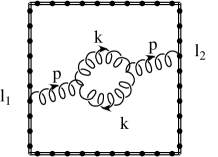
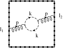
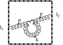
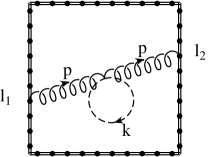
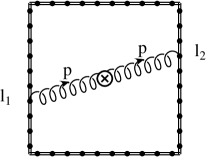
Figure 2: Pure gauge one-loop [${\mathcal{O}}(g^{4})$] vacuum polarization contribution to the Wilson loop. This is the sum of continuum like three-gluon and ghost-ghost-gluon couplings, and both a continuum like four-gluon tadpole contribution and lattice specific four-gluon and two-ghost-two-gluon tadpole pieces. The last measure diagram is due to the Jacobian involved in changing variables in the path integral from $U_{l}$ to $A_{l}$.

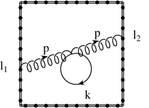
Figure 3: The leading $n_{f}$ contribution arises at ${\mathcal{O}}(g^{4})$ through the fermionic contribution to the vacuum polarization, and the lattice specific fermionic tadpole contribution.

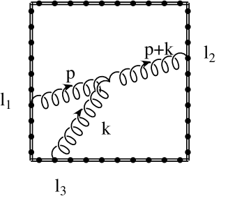
Figure 4: The ${\mathcal{O}}(g^{4})$ spider contribution to the Wilson loop.

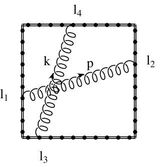
Figure 5: One-loop [${\mathcal{O}}(g^{4})$] two-gluon exchange contribution to the Wilson loop. One part of this diagram is accompanied by a $C_{F}^{2}/2$ colour factor, that arises when exponentiating the tree-level contribution. The remainder is proportional to $C_{F}N/2$ and specific to non-Abelian gauge theories.

The expectation values in the above formulae depend on $g^{2}$ and are sums of gluonic position space $n$-point functions. The leading order [${\mathcal{O}}(g^{2})$] contribution to the Wilson loop is the sum of tree-level two-point functions depicted in Fig. 1. This is easily expressed in momentum space as a sum of phase factors multiplying the momentum space propagator:

$$W_{2} = \sum_{l_{1},l_{2}}\int_{-\pi/a}^{\pi/a}\frac{d^{4}k}{(2\pi)^{4}}\frac{a^{2}}{2N}\mbox{tr}\,T^{a}T^{b}e^{ik[x_{2}-x_{1}+\frac{a}{2}(\hat{\mu}_{2}-\hat{\mu}_{1})]}$$ (7)

$$\times\langle A^{a}_{\mu_{1}}(-k)A^{b}_{\mu_{2}}(k)\rangle$$

$$= W_{2}^{(0)}+g^{2}W_{2}^{(2)}+{\mathcal{O}}(g^{4}).$$

For the Wilson gauge action the gluon propagator reads,

$$\langle A^{a}_{\mu_{1}}(-k)A^{b}_{\mu_{2}}(k)\rangle=\frac{\delta^{ab}(\delta_{\mu_{1},\mu_{2}}-\delta_{\mu_{1},-\mu_{2}})}{\hat{k}^{2}}+\Pi^{ab}_{\mu_{1}\mu_{2}}(k),$$ (8)

where $\hat{k}_{\mu}=2a^{-1}\sin\left(k_{\mu}a/2\right)$ and $\Pi$ is of order $g^{2}$. The colour trace then results in the Casimir factor of the fundamental representation, $C_{F}=\frac{1}{N}\mbox{tr}\,T^{a}T^{a}=(N^{2}-1)/(2N)$. All formulae in this Section as well as in Sec. III below apply to the general $SU(N)$ case unless stated otherwise. In addition the constants $C_{F}$ are factorized out in such a way that the results apply to external sources in any representation $D$ of the gauge group, under the replacement $C_{F}\mapsto C_{D}$.

In explicitly summing the above phase factors one easily obtains the well known tree-level expressions for planar Wilson loops. The vacuum polarization tensor $\Pi$ has to be considered to leading order for an ${\mathcal{O}}(g^{4})$ evaluation of Wilson loops which requires $W_{2}^{(2)}$. The relevant graphs for the gluonic sector are depicted in Fig. 2. The fourth diagram involving a two-gluon-two-ghost vertex (which is lattice specific) as well as a lattice contribution to the four-gluon vertex of the third diagram, result in a lattice tadpole correction to $W_{2}^{(2)}$ that is exactly $(2N^{2}-3)/(24N)$ times the tree-level value $W_{2}^{(0)}$. The two additional diagrams of Fig. 3 have to be considered in the case of dynamical fermions.

To the order at which we are working throughout this paper, $W_{3}$ only contributes through its contraction with the three gluon vertex, depicted in Fig. 4, and we write

$$W_{3}=gW_{3}^{(1)}+{\mathcal{O}}(g^{3}).$$ (9)

In momentum space the phase factor associated with a typical entry in the sum Eq. (II.1) is

$$\int_{-\pi/a}^{\pi/a}\frac{d^{4}kd^{4}k^{\prime}}{(2\pi)^{8}}\frac{i}{N}\mbox{tr}\,T^{a}T^{b}T^{c}e^{ik[x_{2}-x_{1}+\frac{a}{2}(\hat{\mu}_{2}-\hat{\mu}_{1})]}$$ (10)

$$\times e^{ik^{\prime}[x_{3}-x_{1}+\frac{a}{2}(\hat{\mu}_{3}-\hat{\mu}_{1})]}\langle A^{a}_{\mu_{1}}(-k-k^{\prime})A^{b}_{\mu_{2}}(k)A^{c}_{\mu_{3}}(k^{\prime})\rangle.$$

The term

$$W_{4}=W_{4}^{(0)}+{\mathcal{O}}(g^{2})$$ (11)

only contributes to the Wilson loop at ${\mathcal{O}}(g^{4})$ through its contraction with double gluon exchanges, as depicted in Fig. 5. The generic phase factor associated with this diagram is given below, where due to the lack of an appropriately symmetrized contracting vertex we perform the Wick contraction manually, preserving the ordering of colour factors:

$$\int_{-\pi/a}^{\pi/a}\frac{d^{4}k}{(2\pi)^{4}}\frac{d^{4}k^{\prime}}{(2\pi)^{4}}\frac{i}{N}\mbox{tr}\,T^{a}T^{b}T^{c}T^{d}\left\{\begin{array}[]{c}e^{ik[x_{2}-x_{1}+\frac{a}{2}(\hat{\mu}_{2}-\hat{\mu}_{1})]}e^{ik^{\prime}[x_{4}-x_{3}+\frac{a}{2}(\hat{\mu}_{4}-\hat{\mu}_{3})]}\langle A^{a}_{\mu_{1}}(-k)A^{b}_{\mu_{2}}(k)A^{c}_{\mu_{3}}(-k^{\prime})A^{d}_{\mu_{4}}(k^{\prime})\rangle\\ e^{ik[x_{3}-x_{1}+\frac{a}{2}(\hat{\mu}_{3}-\hat{\mu}_{1})]}e^{ik^{\prime}[x_{4}-x_{2}+\frac{a}{2}(\hat{\mu}_{4}-\hat{\mu}_{2})]}\langle A^{a}_{\mu_{1}}(-k)A^{b}_{\mu_{2}}(-k^{\prime})A^{c}_{\mu_{3}}(k)A^{d}_{\mu_{4}}(k^{\prime})\rangle\\ e^{ik[x_{3}-x_{2}+\frac{a}{2}(\hat{\mu}_{3}-\hat{\mu}_{2})]}e^{ik^{\prime}[x_{4}-x_{1}+\frac{a}{2}(\hat{\mu}_{4}-\hat{\mu}_{1})]}\langle A^{a}_{\mu_{1}}(-k^{\prime})A^{b}_{\mu_{2}}(-k)A^{c}_{\mu_{3}}(k)A^{d}_{\mu_{4}}(k^{\prime})\rangle\end{array}\right\}.$$ (12)

After evaluating colour traces, this term can be split into an “Abelian” and a “non-Abelian” part. The Abelian part is proportional to $C_{F}^{2}/2$ and can be obtained by expanding $\exp(-g^{2}W_{2})$. The remainder is specific to non-Abelian gauge theories and proportional to $C_{F}N/2$, the same colour factor that also accompanies the vacuum polarization diagrams.

The integrands were coded with the help of a C++ package written by one of the authors, and then integrated using VEGAS Lepage:1978sw . For finite Wilson loops to ${\mathcal{O}}(g^{2})$ and ${\mathcal{O}}(g^{4})$ we compute 4 and 8 dimensional momentum integrals, respectively. In the case of the potential one can analytically perform the limit $T\to\infty$. This allows us to compute the momentum integrals in one less dimension, leaving 3 and 7 dimensional integrals.

The fermionic Wilson-SW and KS vacuum polarization graphs have been computed after a further analytical integration over the 4-component of the internal loop momentum, leaving a 6 dimensional integration to be performed in the cases of the potential and the static self energy.

It is relatively easy to automate the generation of the phase factors that are required for arbitrary curves ${\mathcal{C}}$. We generate the perturbative expansion for both small rectangular Wilson loops and for the non-planar loops shown in Fig. 6. We refer to these non-planar loops as the chair and the (three-dimensional) “parallelogram”; both are contained within the unit cube and are used within certain improved gauge actions.

Figure 6: The non-planar Wilson loops in the unit cube which we refer to as the chair and the “parallelogram”, respectively.

II.2 Definitions

We write the tree-level contribution to the expansion of the Wilson loop with the Wilson gauge action as,

$$W_{2}^{(0)}=C_{F}W_{T}.$$ (13)

For Wilson and SW fermions with the Wilson gauge action we write the vacuum polarization insertions as,

$$W_{2}^{(2)}=C_{F}\left(\frac{N}{2}W_{\Pi}+\frac{2N^{2}-3}{24N}W_{T}+n_{f}X_{f}\right).$$ (14)

For Wilson-SW fermions we define,

$$X_{f}=X_{f}^{(0)}+X_{f}^{(1)}c_{SW}+X_{f}^{(2)}c_{SW}^{2},$$ (15)

where $c_{SW}=0$ in the Wilson case and $c_{SW}=1+{\mathcal{O}}(g^{2})$ in the SW case. The $X_{f}$ will depend on the quark mass in lattice units $ma$. In the case of Wilson-SW fermions and the order of perturbation theory we are working at we have, $ma=m_{0}a=(\kappa^{-1}-\kappa^{-1}_{c})/2$. As anticipated above, we have factorized out a lattice tadpole term that is proportional to $W_{T}$. For KS fermions we define analogously,

$$X_{f}=X_{f}^{(KS)}.$$ (16)

In this case $n_{f}$ has to be a multiple of four. For each of the above quantities we may write a similar expansion in terms of $\alpha_{L}=g^{2}/(4\pi)$, rather than $g^{2}$, with lower case coefficients $w$ and $x$, where $w_{T}=4\pi W_{T}$, $w_{\Pi}=(4\pi)^{2}W_{\Pi}$, $x=(4\pi)^{2}X$ and so forth.

We denote the spider contribution by,

$$W_{3}^{(1)}=\frac{C_{F}N}{2}W_{S}.$$ (17)

The double gluon exchange can be written as the sum of Abelian and non-Abelian pieces, where the Abelian piece is the next term in the exponentiation of the tree-level contribution,

$$W_{4}^{(0)}=-\frac{C_{F}^{2}}{2}W_{T}^{2}+\frac{C_{F}N}{2}W_{NA}.$$ (18)

In combining the above Eqs. (13) – (18) with Eqs. (3), (7), (9) and (11), we obtain the expansion of the Wilson loop,

$$W=1-W_{\mbox{\scriptsize LO}}g^{2}-\left(W_{\mbox{\scriptsize NLO}}+C_{F}n_{f}X_{f}\right)g^{4},$$ (19)

where

$$W_{\mbox{\scriptsize LO}} = C_{F}W_{T},$$ (20)

$$W_{\mbox{\scriptsize NLO}} = C_{F}\left(\frac{N}{2}W_{\Sigma}+\frac{2N^{2}-3}{24N}W_{T}-\frac{C_{F}}{2}W_{T}^{2}\right),$$ (21)

$$W_{\Sigma} = W_{\Pi}+W_{NA}+W_{S}$$ (22)

The $W_{T}^{2}$ term within Eq. (21) originates from the exponentiation of the Abelian part of the one gluon exchange, Eq. (18). It is cancelled in the Taylor expansion of $\ln W$, which turns out to be proportional to $C_{F}$, at least to ${\mathcal{O}}(g^{4})$. The latter observation, which is referred to as the “Casimir scaling” hypothesis in the literature (see e.g. Refs. Bali:2000un ; Deldar:2000vi ), implies that, for given $N$ and $n_{f}$, $\ln W$ only depends on the representation of the static colour sources, $D$, through its proportionality to the corresponding Casimir charge $C_{D}=(\mbox{tr}\,T^{a}_{D}T^{a}_{D})/\mbox{dim}_{D}$. Note that in the case of the fundamental representation, by using the relation $C_{F}=(N^{2}-1)/(2N)$, Eq. (21) can be rearranged into the form,

$$W_{\mbox{\scriptsize NLO}}=(N^{2}-1)\left(W_{a}+\frac{1}{N^{2}}W_{b}\right),$$ (23)

where

$$W_{a} = \frac{1}{24}\left(6W_{\Sigma}+W_{T}-3W_{T}^{2}\right),$$ (24)

$$W_{b} = \frac{1}{16}\left(-W_{T}+2W_{T}^{2}\right).$$ (25)

For improved gluonic actions Eq. (21) does not apply and hence $W_{a}$ and $W_{b}$ can take somewhat different forms. The factorization Eq. (23) is frequently employed throughout the literature, e.g. in Refs. DiGiacomo:1981wt ; Iso:1987dj ; Alles:1994dn .

II.3 Small Wilson loop results

The pure gauge results on small Wilson loops for the Wilson gluonic action are displayed in Tab. 1. We reproduce the known plaquette results of Di Giacomo and Rossi DiGiacomo:1981wt and Allés et al. Alles:1998is and the small planar Wilson loop results of Wohlert, Weisz and Wetzel Weisz:1984bn . Boldface values have been calculated by us for the first time. We also calculated tree-level Wilson loops for the Symanzik-Weisz (SyW) Weisz:1983zw and Iwasaki (I) Iwasaki:1984cj actions. These results are displayed in Tabs. 2 and 3, respectively, together with the ${\mathcal{O}}(g^{4})$ values of Iso and Sakai Iso:1987dj (italicized) which we have not validated ourselves.

Table 1: Pure gauge Wilson loops with the Wilson gauge action. The different contributions are defined in Eqs. (19) – (22). The values $W_{\mbox{\scriptsize NLO}}$ apply to Wilson loops in the fundamental representation of $SU(3)$ gauge theory. Boldface values are calculated here for the first time.

loop	$W_{T}$	$W_{\Sigma}$	$W_{\mbox{\scriptsize NLO}}$
$1\times 1$	0.25	0.0100109(4)	0.033911(1)
chair	0.3922(1)	0.02204(2)	0.01629(1)
parall.	0.4267(1)	0.02730(2)	0.01128(1)
$1\times 2$	0.43110(6)	0.02463(2)	0.00382(1)
$2\times 2$	0.68466(8)	0.05303(2)	-0.12043(9)

Table 2: Pure gauge Wilson loop results with the Symanzik-Weisz action. Italicized values have been obtained in Ref. Iso:1987dj . $W_{a}$ and $W_{b}$ are defined in Eq. (23) and $W_{\mbox{\scriptsize NLO}}$ applies to $N=3$.

loop	$W_{T}^{SyW}$	$W_{a}^{SyW}$	$W_{b}^{SyW}$	$W_{\mbox{\scriptsize NLO}}^{SyW}$
$1\times 1$	0.18313(1)	-0.001133	0.001333	-0.00788
chair	0.28850(8)	—	—	—
parall.	0.3162(1)	—	—	—
$1\times 2$	0.33130(6)	-0.00678	0.00830	-0.0469

We are able to reproduce the known contributions to the plaquette for massless KS Heller:1985eq and Wilson Hamber:1983ft quarks with increased precision. The calculation of the SW contribution, as well as all results for massive quarks are new. We also calculate the one-loop $n_{f}$ piece of the plaquette with the Iwasaki gauge action which has been used, for instance, in the dynamical fermion simulations of the CP-PACS group Yoshie:2000wd . We display a selection of $m=0$ results in Tab. 4. In Fig. 7 we show the mass dependence of $X_{f}$ for the case of the Wilson gluonic action, combined with all three different fermionic actions. The open symbols correspond to the respective $m=0$ limits. The numbers that are plotted in the figure are also displayed in Tab. 5.

Table 3: The same as Tab. 2 for the Iwasaki gauge action.

loop	$W_{T}^{I}$	$W_{a}^{I}$	$W_{b}^{I}$	$W_{\mbox{\scriptsize NLO}}^{I}$
$1\times 1$	0.10514(2)	-0.002269	0.003142	-0.01536
chair	0.16676(4)	—	—	—
parall.	0.18494(4)	—	—	—
$1\times 2$	0.20166(4)	-0.00653	0.00881	-0.04441

Table 4: Massless fermionic contribution to Wilson loops for the different quark actions. The plaquette is displayed for both Wilson (W) and Iwasaki (I) gluonic actions. All other loops are just shown for the Wilson gauge action. $X_{f}$ are defined in Eqs. (14), (16) and (19).

loop	$X_{f}^{(KS)}/10^{-3}$	$X_{f}^{(0)}/10^{-3}$	$X_{f}^{(1)}/10^{-3}$	$X_{f}^{(2)}/10^{-3}$
W: $1\times 1$	-1.2258(7)	-1.392(3)	0.0404(5)	-1.1927(2)
I: $1\times 1$	-0.2592(4)	-0.294(2)	0.00156(2)	-0.3396(2)
chair	-2.674(2)	-2.974(7)	0.0724(9)	-1.9672(6)
parall.	-2.890(2)	-3.31(1)	0.101(1)	-2.3248(6)
$1\times 2$	-2.357(1)	-2.652(6)	0.113(1)	-2.9518(6)
$2\times 2$	-4.113(3)	-4.76(2)	0.322(2)	-6.684(1)

Table 5: Mass dependence of the fermionic contribution to the plaquette for the Wilson gluonic action.

$ma$	$X_{f}^{(KS)}/10^{-3}$	$X_{f}^{(0)}/10^{-3}$	$X_{f}^{(1)}/10^{-3}$	$X_{f}^{(2)}/10^{-3}$
0.00	-1.2258(7)	-1.392(3)	0.0404(5)	-1.1927(2)
0.05	-1.2211(7)	-1.275(2)	0.0267(5)	-1.1769(2)
0.10	-1.2076(6)	-1.176(2)	0.0154(5)	-1.1603(2)
0.20	-1.1576(6)	-1.006(2)	-0.0011(4)	-1.1256(2)
0.50	-0.8954(5)	-0.655(2)	-0.0207(3)	-1.0158(2)
1.00	-0.4617(4)	-0.359(2)	-0.0208(2)	-0.8455(1)
2.00	-0.1091(2)	-0.141(1)	-0.0104(1)	-0.5967(1)
4.00	-0.01212(6)	-0.038(1)	-0.00261(4)	-0.33661(4)
8.00	-0.00093(2)	-0.0070(6)	-0.00034(1)	-0.14920(2)

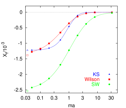
Figure 7: $n_{f}$ contributions to the one-loop plaquette for KS, Wilson, and SW quarks. All $X_{f}$ interpolate smoothly between the massless values (open symbols) and zero as the quark mass is increased.

In the region $ma<0.25$, which is most relevant for lattice simulations, this dependence is relatively weak and can be parametrized by,

$$X_{f}(ma)=X_{f}(0)+b\,ma+c(ma)^{2},$$ (26)

with $X_{f}(0)$ as in the first row of Tab. 5 and $b\approx 0$, 0.0024 and 0.0024 and $c\approx 0.0017$, $-0.0023$ and $-0.0017$ for KS, Wilson and SW fermions, respectively. As expected the mass dependence remains weak for any Wilson loop with linear dimensions that are small compared to the inverse quark mass.

III The perturbative static potential

After a historical survey of the existing literature we will briefly explain our method and the notations that we adopt, before presenting results on the ${\mathcal{O}}(g^{4})$ potential. We will then discuss limiting cases, including the continuum limit and lattice artefacts as well as mass dependent terms in the conversion between lattice and $\overline{MS}$ schemes at finite lattice spacing. We conclude with paragraphs on the perturbative $\beta$-shift, boosted lattice perturbation theory and the static source self energy.

III.1 The method and definitions

The one-loop potential has first been calculated for pure $SU(2)$ gauge theory by Müller and Rühl MullerRuhl . Subsequently, a closed formula for pure $SU(N)$ gauge theory with the standard Wilson as well as Symanzik improved gauge actions was derived by Weisz and Wohlert Weisz:1984bn . The coefficients of the perturbative expansion have first been evaluated numerically by Altevogt and Gutbrod Altevogt:1995cj for $SU(2)$ pure gauge theory with Wilson glue on isotropic and anisotropic lattices.

Here we restrict our calculations to the case of the Wilson gauge action on an isotropic lattice but include massive Wilson, SW and KS fermions as well as $N>2$. We also improve the numerical precision with respect to earlier results and incorporate off-axis lattice separations ${\mathbf{R}}$ of the colour sources. We define the static potential,

$$aV({\mathbf{R}}a) = -\lim_{T\rightarrow\infty}\frac{d\ln W({\mathbf{R}},T)}{dT}$$ (27)

$$= V_{1}({\mathbf{R}})g^{2}+V_{2}({\mathbf{R}})g^{4}+\cdots$$ (28)

$$= v_{1}({\mathbf{R}})\alpha_{L}+v_{2}({\mathbf{R}})\alpha_{L}^{2},$$ (29)

where $\alpha_{L}=g^{2}/(4\pi)$, $v_{i}({\mathbf{R}})=(4\pi)^{i}V_{i}({\mathbf{R}})$. $W({\mathbf{R}},T)$ denotes a (generalized) rectangular Wilson loop with the temporal extent of $T$ lattice units. The expansion of the potential in terms of $g^{2}$ is suitable for calculations in lattice perturbation theory and for the comparison with data from lattice simulations, while the expansion in terms of $\alpha_{L}$ turns out to be more convenient to relate our results to those obtained in a continuum scheme.

The only gluon exchanges that contribute to the $T$ dependence of $W({\mathbf{R}},T)$ in the limit $T\rightarrow\infty$ [at least up to ${\mathcal{O}}(g^{6})$] are those between temporal lines of a Wilson loop. After exploiting translational invariance in time, Eqs. (7) and (8) result in,

$$V_{1}({\mathbf{R}})=C_{F}\int\frac{d^{3}\!q}{(2\pi)^{3}}\frac{2\sin^{2}\left(\frac{{\mathbf{q}}{\mathbf{R}}a}{2}\right)}{\hat{\mathbf{q}}^{2}}.$$ (30)

The ${\mathcal{O}}(g^{4})$ coefficient $V_{2}$ consists of two parts: one contribution from $W_{2}$, i.e. the vacuum polarization tensor $\Pi$, inserted into Eq. (30), and a second contribution that originates from the “non-Abelian” part $W_{NA}$ of $W_{4}$ [Eq. (18)]. The spider diagrams, $W_{3}$, do not contribute to $V({\mathbf{R}})$ at this order. A closed formula for $V_{2}$ can be found in Ref. Weisz:1984bn , and we extend this calculation by incorporating the fermionic contributions to the vacuum polarization tensor. In our calculation we produce $V_{2}$ automatically from the Feynman rules and find agreement with the published analytic form.

The potential can be factorized into an interaction part and a part that is due to the static source self energy, $V_{S}=2\delta m_{\mbox{\scriptsize stat}}$,

$$V({\mathbf{R}}a)=V_{\mbox{\scriptsize int}}({\mathbf{R}}a)+V_{S}.$$ (31)

Since in perturbation theory $V_{\mbox{\scriptsize int}}\rightarrow 0$ as $r\rightarrow\infty$ we can identify the self energy $V_{S}$ with $\lim_{r\rightarrow\infty}V(r)$ and write,

$$aV_{S} = V_{1}(\infty)g^{2}+V_{2}(\infty)g^{4}+\cdots,$$ (32)

$$aV_{\mbox{\scriptsize int}}({\mathbf{R}}a) = V_{L,1}({\mathbf{R}})g^{2}+V_{L,2}({\mathbf{R}})g^{4}+\cdots,$$ (33)

where $V_{L,i}({\mathbf{R}})=V_{i}({\mathbf{R}})-V_{i}(\infty)$. The limit $R\rightarrow\infty$ can easily be realized by replacing the factors $\sin^{2}[{\mathbf{q}}{\mathbf{R}}a/2]=[1-\cos({\mathbf{q}}{\mathbf{R}}a)]/2$ within the external 3-dimensional Fourier transformations in the expressions for $V_{1}$ [cf. Eq. (30)] and $V_{2}$ by the constant value $1/2$.

Table 6: Gluonic contributions to the static potential, [see Eqs. (34) – (III.1)]. The last line ($R=\infty$) contains the respective contributions to the static self energy $aV_{S}$. The values for $V_{2}$ in the last column only apply to the case $N=3,n_{f}=0$.

${\mathbf{R}}$	$V_{T}/10^{-2}$	$V_{\Pi}/10^{-2}$	$V_{NA}/10^{-2}$	$V_{2}/10^{-2}$
(1,0,0)	16.6667	1.1920 (1)	0.1499 (1)	7.3134 (3)
(2,0,0)	20.9842	1.6316 (2)	0.5470 (2)	10.1862 (6)
(3,0,0)	22.5186	1.8062 (3)	0.7435 (3)	11.3546 (8)
(4,0,0)	23.2442	1.8993 (5)	0.8526 (3)	11.9605(11)
(5,0,0)	23.6630	1.9608 (6)	0.9194 (4)	12.3335(14)
(6,0,0)	23.9366	2.0028 (7)	0.9663 (4)	12.5873(17)
(7,0,0)	24.1300	2.0345 (9)	1.0012 (5)	12.7740(19)
(8,0,0)	24.2742	2.0585(10)	1.0288 (5)	12.9176(22)
(1,1,0)	19.7540	1.4532 (1)	0.4186 (1)	9.2308 (4)
(1,1,1)	20.9152	1.5697 (2)	0.5443 (2)	10.0378 (5)
(2,1,0)	21.6800	1.6853 (2)	0.6337 (2)	10.6602 (7)
(2,1,1)	22.0766	1.7253 (3)	0.6858 (2)	10.9546 (7)
(2,2,0)	22.4676	1.7827 (3)	0.7384 (3)	11.2833 (8)
(2,2,1)	22.6572	1.8034 (4)	0.7647 (3)	11.4297 (9)
(2,2,2)	23.0080	1.8527 (4)	0.8163 (3)	11.7292(10)
(3,3,0)	23.4016	1.9153 (5)	0.8776 (4)	12.0863(12)
(4,2,0)	23.4889	1.9266(52)	0.8914(11)	12.1607(81)
(4,2,2)	23.6538	1.9530 (6)	0.9186 (4)	12.3137(15)
(3,3,3)	23.7512	1.9679 (7)	0.9345 (4)	12.4023(15)
(4,4,0)	23.8686	1.9884 (7)	0.9546 (4)	12.5162(16)
(4,4,2)	23.9512	2.0011 (8)	0.9695 (4)	12.5944(17)
(4,4,4)	24.1286	2.0310 (9)	1.0018 (5)	12.7675(20)
$\infty$	25.2731	$\sum:$ 3.5459(15)		14.1122 (31)

Table 7: Fermionic contributions to the static potential $V_{f}$ [see Eqs. (III.1) and (36)] for massless KS [$V_{f}^{(KS)}$] and Wilson-SW [$V_{f}^{(i)}$, see Eq. (36)] quarks.

${\mathbf{R}}$	$V_{f}^{(KS)}/10^{-3}$	$V_{f}^{(0)}/10^{-3}$	$V_{f}^{(1)}/10^{-3}$	$V_{f}^{(2)}/10^{-3}$
(1,0,0)	-1.0830 (1)	-1.1318 (1)	0.0563 (2)	-1.5070 (1)
(2,0,0)	-1.4893 (3)	-1.6698 (1)	0.1469 (3)	-2.6859(16)
(3,0,0)	-1.7004 (5)	-1.9272 (2)	0.1978 (3)	-3.0033 (3)
(4,0,0)	-1.8123 (7)	-2.0723 (2)	0.2331(34)	-3.1578 (3)
(5,0,0)	-1.8900 (9)	-2.1659 (2)	0.2479 (4)	-3.2589 (3)
(6,0,0)	-1.9427(11)	-2.2328 (3)	0.2611 (4)	-3.3294 (4)
(7,0,0)	-1.9851(13)	-2.2818 (3)	0.2706 (4)	-3.3840 (4)
(8,0,0)	-2.0155(16)	-2.3207 (3)	0.2779 (5)	-3.4234 (4)
(1,1,0)	-1.3418 (2)	-1.4784 (1)	0.0970 (2)	-2.0409 (2)
(1,1,1)	-1.4609 (3)	-1.6415 (1)	0.1252 (3)	-2.3156 (2)
(2,1,0)	-1.5687 (4)	-1.7723 (1)	0.1637 (3)	-2.6703 (3)
(2,1,1)	-1.6169 (4)	-1.8383 (2)	0.1755 (4)	-2.7298 (3)
(2,2,0)	-1.6774 (5)	-1.9121 (2)	0.1944 (4)	-2.8773 (3)
(2,2,1)	-1.7043 (5)	-1.9474 (2)	0.2010 (4)	-2.9099 (3)
(2,2,2)	-1.7615 (6)	-2.0182 (2)	0.2171 (4)	-3.0166 (4)
(3,3,0)	-1.8355 (8)	-2.1045 (2)	0.2366 (5)	-3.1557 (4)
(4,2,0)	-1.8499 (9)	-2.1233(11)	0.2389(10)	-3.1917 (8)
(4,2,2)	-1.8824 (9)	-2.1624 (3)	0.2476 (5)	-3.2294 (4)
(3,3,3)	-1.9005(10)	-2.1852 (3)	0.2526 (5)	-3.2536 (5)
(4,4,0)	-1.9269(11)	-2.2144 (3)	0.2584 (5)	-3.2955 (5)
(4,4,2)	-1.9428(12)	-2.2351 (3)	0.2624 (5)	-3.3180 (5)
(4,4,4)	-1.9804(14)	-2.2810 (3)	0.2714 (5)	-3.3720 (5)
$\infty$	-2.3359 (4)	-2.6808 (4)	0.3266(10)	-3.7174(12)

Table 8: Fermionic contributions to the static potential for massive KS and Wilson-SW quarks.

${\mathbf{R}}$	$ma$	$V_{f}^{(KS)}/10^{-3}$	$V_{f}^{(0)}/10^{-3}$	$V_{f}^{(1)}/10^{-3}$	$V_{f}^{(2)}/10^{-3}$
	0	-1.0830(1)	-1.1318(1)	0.0563(2)	-1.5070(1)
	0.01	-1.0828(1)	-1.1120(1)	0.0525(4)	-1.5034(2)
	0.03	-1.0811(1)	-1.0733(1)	0.0437(4)	-1.4952(2)
(1,0,0)	0.04	-1.0789(2)	-1.0545(1)	0.0396(4)	-1.4911(2)
	0.05	-1.0777(1)	-1.0360(1)	0.0357(4)	-1.4869(2)
	0.10	-1.0627(1)	-0.9491(1)	0.0177(2)	-1.4650(1)
	0.25	-0.9720(1)	-0.7374(1)	-0.0142(1)	-1.3966(1)
	0	-1.3418(2)	-1.4784(1)	0.0970(2)	-2.0409(2)
	0.01	-1.3416(2)	-1.4517(1)	0.0893(2)	-2.0360(2)
	0.03	-1.3394(2)	-1.3997(1)	0.0754(2)	-2.0254(2)
(1,1,0)	0.04	-1.3367(4)	-1.3743(1)	0.0685(2)	-2.0202(1)
	0.05	-1.3349(2)	-1.3495(1)	0.0623(3)	-2.0147(2)
	0.10	-1.3151(2)	-1.2324(1)	0.0347(2)	-1.9871(1)
	0.25	-1.1980(2)	-0.9489(1)	-0.0168(2)	-1.8976(1)
	0	-1.4609(3)	-1.6415(1)	0.1252(3)	-2.3156(2)
	0.01	-1.4607(3)	-1.6114(1)	0.1157(3)	-2.3099(2)
	0.03	-1.4580(3)	-1.5525(1)	0.0977(3)	-2.2985(2)
(1,1,1)	0.04	-1.4555(5)	-1.5238(2)	0.0894(2)	-2.2926(1)
	0.05	-1.4530(3)	-1.4958(1)	0.0812(3)	-2.2868(2)
	0.10	-1.4306(3)	-1.3635(1)	0.0462(3)	-2.2563(2)
	0.25	-1.2990(3)	-1.0441(1)	-0.0182(3)	-2.1567(2)
	0	-1.4893(3)	-1.6698(1)	0.1469(3)	-2.6859(16)
	0.01	-1.4889(3)	-1.6391(1)	0.1368(7)	-2.6778 (5)
	0.03	-1.4863(3)	-1.5789(1)	0.1155(7)	-2.6644(5)
(2,0,0)	0.04	-1.4831(5)	-1.5496(1)	0.1057(7)	-2.6576(5)
	0.05	-1.4813(3)	-1.5209(1)	0.0961(7)	-2.6508(5)
	0.10	-1.4582(3)	-1.3855(1)	0.0539(3)	-2.6146(2)
	0.25	-1.3242(3)	-1.0586(1)	-0.0214(3)	-2.4994(2)
	0	-1.5687(4)	-1.7723(1)	0.1637(3)	-2.6703(3)
	0.01	-1.5684(4)	-1.7393(2)	0.1512(3)	-2.6641(2)
	0.03	-1.5654(4)	-1.6748(1)	0.1283(3)	-2.6511(3)
(2,1,0)	0.04	-1.5615(6)	-1.6433(2)	0.1172(3)	-2.6460(5)
	0.05	-1.5596(4)	-1.6125(1)	0.1071(3)	-2.6380(3)
	0.10	-1.5345(4)	-1.4671(1)	0.0621(3)	-2.6038(3)
	0.25	-1.3883(4)	-1.1170(1)	-0.0198(3)	-2.4912(2)

Table 9: Tab. 8 continued.

${\mathbf{R}}$	$ma$	$V_{f}^{(KS)}/10^{-3}$	$V_{f}^{(0)}/10^{-3}$	$V_{f}^{(1)}/10^{-3}$	$V_{f}^{(2)}/10^{-3}$
	0	-1.6169(4)	-1.8383(2)	0.1755(4)	-2.7298(3)
	0.01	-1.6164(4)	-1.8039(2)	0.1623(3)	-2.7233(2)
	0.03	-1.6132(4)	-1.7364(1)	0.1374(4)	-2.7104(3)
(2,1,1)	0.04	-1.6099(6)	-1.7033(2)	0.1257(3)	-2.7037(2)
	0.05	-1.6072(4)	-1.6712(2)	0.1145(4)	-2.6971(3)
	0.10	-1.5801(4)	-1.5192(1)	0.0664(4)	-2.6624(3)
	0.25	-1.4269(4)	-1.1536(1)	-0.0208(3)	-2.5479(3)
	0	-1.6774(5)	-1.9121(2)	0.1944(4)	-2.8773(3)
	0.01	-1.6768(5)	-1.8760(2)	0.1794(4)	-2.8706(3)
	0.03	-1.6735(5)	-1.8052(2)	0.1520(4)	-2.8569(3)
(2,2,0)	0.04	-1.6694(7)	-1.7705(2)	0.1388(4)	-2.8500(3)
	0.05	-1.6668(5)	-1.7366(2)	0.1266(4)	-2.8431(3)
	0.10	-1.6380(5)	-1.5768(1)	0.0729(4)	-2.8066(3)
	0.25	-1.4754(5)	-1.1931(1)	-0.0228(3)	-2.6864(3)
	0	-1.7004(5)	-1.9272(2)	0.1978(3)	-3.0033(3)
	0.01	-1.7001(5)	-1.8907(2)	0.1837(8)	-2.9979(6)
	0.03	-1.6963(5)	-1.8192(2)	0.1550(8)	-2.9832(6)
(3,0,0)	0.04	-1.6923(6)	-1.7842(2)	0.1416(9)	-2.9758(6)
	0.05	-1.6893(5)	-1.7499(2)	0.1289(9)	-2.9682(6)
	0.10	-1.6595(5)	-1.5883(1)	0.0718(3)	-2.9282(2)
	0.25	-1.4922(5)	-1.2006(1)	-0.0269(3)	-2.8014(2)
	0	-1.7043(5)	-1.9474(2)	0.2010(4)	-2.9099(3)
	0.01	-1.7036(5)	-1.9104(2)	0.1858(3)	-2.9033(2)
	0.03	-1.7003(5)	-1.8379(2)	0.1567(4)	-2.8894(3)
(2,2,1)	0.04	-1.6975(7)	-1.8024(2)	0.1435(3)	-2.8826(2)
	0.05	-1.6932(5)	-1.7678(2)	0.1306(4)	-2.8754(3)
	0.10	-1.6629(5)	-1.6041(1)	0.0751(4)	-2.8387(3)
	0.25	-1.4954(5)	-1.2118(1)	-0.0236(3)	-2.7174(3)
	0	-2.3333(4)	-2.6808(4)	0.3266(10)	-3.7174(12)
	0.01	-2.300 (6)	-2.6123(3)	0.2978 (2)	-3.7080(20)
	0.03	-2.284 (6)	-2.4805(3)	0.2432 (4)	-3.6886 (4)
$\infty$	0.04	-2.256 (5)	-2.4180(3)	0.2166(12)	-3.6794(10)
	0.05	-2.241 (6)	-2.3582(2)	0.1934(10)	-3.6728 (2)
	0.10	-2.1603(3)	-2.0893(2)	0.0956 (2)	-3.6268 (2)
	0.25	-1.845 (4)	-1.5082(2)	-0.0536(2)	-3.4728 (2)

We write,

$$V_{1}({\mathbf{R}}) = C_{F}V_{T}({\mathbf{R}})$$ (34)

$$V_{2}({\mathbf{R}}) = C_{F}\left\{\frac{N}{2}[V_{\Pi}({\mathbf{R}})+V_{NA}({\mathbf{R}})]\right.$$

$$+\left.\frac{2N^{2}-3}{24N}V_{T}({\mathbf{R}})+n_{f}V_{f}({\mathbf{R}})\right\},$$

where $V_{\Pi}$ denotes the gluonic vacuum polarization and $V_{NA}$ is a contribution, specific to non-Abelian gauge theories, where the ordering of gluon vertices along the Wilson loop has to be considered. In the case of KS quarks we denote the fermionic vacuum polarization contribution to the potential by $V_{f}^{(KS)}$ while for Wilson-SW quarks we split this contribution into three parts,

$$V_{f}({\mathbf{R}})=V_{f}^{(0)}({\mathbf{R}})+c_{SW}V_{f}^{(1)}({\mathbf{R}})+c_{SW}^{2}V_{f}^{(2)}({\mathbf{R}}).$$ (36)

III.2 Results on the potential and violations of rotational symmetry

In Tab. 6 we display $V_{T}$, $V_{\Pi}$ and $V_{NA}$ as well as $V_{2}$ for $N=3,n_{f}=0$ for small on- and off-axis distances ${\mathbf{R}}$. At the origin all $V$ are zero and $V_{T}(1,0,0)=1/6$. In Tab. 7 we display the corresponding results on the different $V_{f}$’s for massless quarks while in Tabs. 8 – 9 the results for distances $R\leq 3$ as well as for $R\rightarrow\infty$ are shown for quarks of various masses.

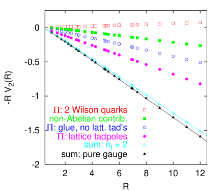
Figure 8: ${\mathcal{O}}(g^{4})$ contribution to the static potential, multiplied by $-R$ for $N=3$. The solid triangles are the sum of the pure gauge contributions: non-Abelian, vacuum polarization and the lattice tadpole contribution to the vacuum polarization. The open triangles incorporate 2 flavours of Wilson fermions.

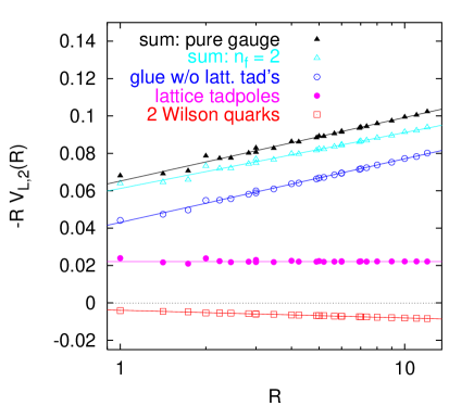
Figure 9: The same as Fig. 8 but with the self energy contribution subtracted, $V_{2,L}(R)=V_{2}(R)-V_{2}(\infty)$, and with a logarithmic scale.

In Fig. 8 we separately display the different ${\mathcal{O}}(g^{4})$ contributions to the quantity $-RV_{2}({\mathbf{R}})$ as a function of $R$. The factor $-R$ results in a cancellation of the leading order Coulomb behaviour. Note that the lattice tadpole contribution to the vacuum polarization (solid circles) is numerically equally important as the sum of the remaining vacuum polarization diagrams and the non-Abelian contribution. As one would naïvely expect, the effect of fermions (open squares) goes into the opposite direction, relative to the pure gauge contributions. In a continuum calculation using dimensional regularization $-RV_{2}({\mathbf{R}})$ contains only a logarithmic dependence on R, but in the lattice calculation the $R$ dependence of the points is dominated by a linear piece arising from the static source self energy contribution to $V_{2}({\mathbf{R}})$, $V_{S,2}=V_{2}(\infty)$. In Fig. 9 we subtract this term, before multiplying the result with $-R$. Note the logarithmic scale. The static source self-energy was previously known to order $\alpha^{2}$ with massless Wilson and SW quarks Martinelli:1999vt and to ${\mathcal{O}}(\alpha^{3})$ in the pure gauge theory DiRenzo:2001nd ; Trottier:2001vj . The mass-dependence, as well as the results for KS sea quarks, are new.

In the limit $r\gg a$, i.e. $R=r/a\gg 1$ rotational symmetry should be restored such that we are able to compare our result to calculations performed in a continuum scheme (continuous curves in Figs. 8 and 9). The potential has been calculated in the $\overline{MS}$ scheme to order $\alpha^{3}$ Schroder:1999vy ; Melles:2000dq . The conversion between the $\overline{MS}$ and the lattice scheme has been worked out to this order too for Wilson-SW fermions Christou:1998ws ; Bode:2001uz (for KS fermions only to ${\mathcal{O}}(\alpha^{2})$ Weisz:1981pu ; Luscher:1995zz ), and $V_{S}$ vanishes by definition to all orders in dimensional regularization. The form of the large $R$ expectation is worked out in Appendix A.4 [Eqs. (192) – (194)]. Here we display the parametrization of the curves in the limit of massless sea quarks:

$$-rV_{L,2}({\mathbf{r}}/a) \stackrel{{\scriptstyle r/a\rightarrow\infty}}{{\longrightarrow}} -rV_{c,2}(r)$$

$$= \frac{C_{F}}{4\pi}\left[b_{1}+a_{1}^{R}+2\beta_{0}\ln(r/a)\right].$$

The constants $b_{1}$ and $a_{1}^{R}=a_{1}+2\gamma\beta_{0}$ are defined in Eqs. (134) and (154), respectively. $b_{1}$ originates from the conversion between the $\overline{MS}$ and the lattice scheme, Eq. (133). The logarithmic running is proportional to the $\beta$-function coefficient $\beta_{0}=(11N-2n_{f})/(12\pi)$.

We can define an effective Coulomb coupling $C_{F}\alpha_{R}$ from the potential:

$$-r\left[V(r)-V_{S}\right] = C_{F}\alpha_{R}\left(r^{-1}\right)$$ (38)

$$= C_{F}\alpha_{L}-RV_{L,2}(R)g^{4}.$$ (39)

Note that in this limit, $C_{F}\alpha_{L}=-RV_{L,1}(R)$. In Fig. 9 the enhancement of this effective coupling, $C_{F}\alpha_{R}$, is demonstrated, relative to the tree-level value as a function of $R$. The points are indeed consistent with the logarithmic running proportional to $2\beta_{0}C_{F}\ln R/(4\pi)$ that is expected from the QCD $\beta$-function, Eq. (121) [as well as from Eq. (III.2) above]. The lattice tadpole terms do not contribute to this running but renormalize the overall value of the coupling. Lattice simulations are usually performed around $g^{2}\approx 1$, where a fit to quenched lattice data Bali:2000vr ; Bali:2000gf yields $e\approx C_{F}\alpha_{R}[1/(3a)]\approx 0.3$. The tree-level expectation in this case, however, is substantially smaller: $C_{F}\alpha_{R}=C_{F}\alpha_{L}\approx 0.106$. As one can read off from the figure, the one-loop value at $R=3$ adds about 0.08 to this, but still the non-perturbative result is underestimated by perturbation theory in terms of the bare coupling $g^{2}$ by more than 30 %. We will discuss the improvement resulting from the use of so-called boosted perturbation theory in Sec. IV.3 below.

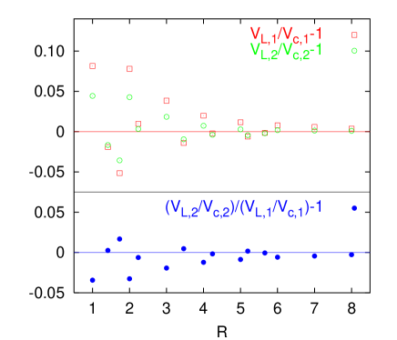
Figure 10: Visualization of lattice artefacts. $V_{L,1}$ and $V_{L,2}$ denote the tree-level and ${\mathcal{O}}(g^{4})$ lattice potentials, where the self energy pieces $V_{i}(\infty)$ have been subtracted. $V_{c,i}$ are the respective large $R$ expectations.

At small $R$ values the lattice results scatter around the continuous curves. We shall investigate these violations of rotational symmetry in more detail: in the top half of Fig. 10 we plot ratios of lattice and continuum ${\mathcal{O}}(g^{2})$ (open squares, $V_{L,1}/V_{c,1}-1$) and ${\mathcal{O}}(g^{4})$ (open circles, $V_{L,2}/V_{c,2}-1$) contributions for on-axis as well as for some off-axis distances ${\mathbf{R}}$ for $n_{f}=0$; the relative violations of rotational symmetry become smaller with bigger $R$ and the one-loop violations are smaller than the tree-level ones. In the lower part of the figure the ratio of the two ratios is displayed, which amounts to replacing the continuum $1/R$ term that multiplies the logarithmic running of $V_{L,2}$ by a lattice “$[1/{\mathbf{R}}]$” function. In doing so we isolate those lattice artefacts that appear specifically at order $g^{4}$; for instance, the lattice tadpole contributions cancel from this combination. The sign is opposite to that of the tree-level differences, which explains the weaker relative violations at ${\mathcal{O}}(g^{4})$ in the comparison with ${\mathcal{O}}(g^{2})$ in the upper part of the figure.

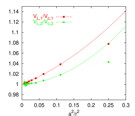
Figure 11: The ratio of lattice and continuum order $\alpha$ and $\alpha^{2}$ pure gauge $SU(3)$ potentials as a function of $a^{2}/r^{2}$ for on-axis separations.

III.3 The continuum limit

The limit of large $R=r/a$ has two interpretations: taken at a fixed lattice spacing $a$ (sufficiently small for perturbation theory still to be reliable at a distance $r$) continuum perturbative predictions should be met. We have already discussed this scenario above and indeed demonstrated this agreement at large $R$ in Figs. 9 and 10. On the other hand taking the limit of large $R$ at fixed physical $r$ corresponds to the continuum limit $a\rightarrow 0$. In Fig. 11 we investigate the approach to the continuum limit by displaying ratios of lattice and continuum perturbation theory results $V_{L,i}/V_{c,i}$ for $i=1,2$ versus $1/R^{2}=a^{2}/r^{2}$ for pure $SU(3)$ gauge theory and on-axis separations $R\geq 2$. For the Wilson gauge action we expect lattice artefacts to be a polynomial in $a^{2}$ and indeed no linear term is found. The solid curves represent fits that are quadratic plus quartic in the lattice spacing $a$. For off-axis separations such as ${\mathbf{R}}\parallel(1,1,0)$ we find a similar picture, but with different $a^{2}$ and $a^{4}$ coefficients.

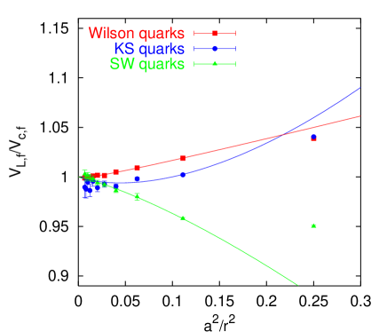
Figure 12: Lattice artefacts on the fermionic contribution to the on-axis potential as a function of $a^{2}/r^{2}$ for different actions of massless quarks. Note that the leading order contribution is proportional to $a/r$ for Wilson fermions.

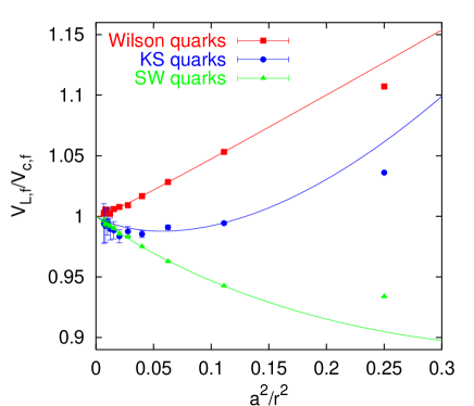
Figure 13: Lattice artefacts on the fermionic contribution to the on-axis potential as a function of $a^{2}/r^{2}$ for $ma=0.1$.

The same comparison is displayed for the fermionic contributions $V_{L,f}({\mathbf{R}})=V_{f}({\mathbf{R}})-V_{f}(\infty)$ and $V_{c,f}(r)=\lim_{a\rightarrow 0}V_{L,f}(r/a)$ alone for massless quarks in Fig. 12. The fit curves are quadratic plus cubic for SW ($c_{SW}=1$ to this order in perturbation theory) and KS fermions while for Wilson fermions we indeed require the expected linear term and attempt a linear plus quadratic fit. The coefficient of the linear term turns out to be so small that the quadratic term already dominates for distances $a/r>0.1$. We see that in spite of the more favourable functional dependence on $a$ the perturbative lattice artefacts of SW fermions are numerically bigger over the whole displayed $R$ range than those of Wilson fermions. However, the KS action “outperforms” both Wilson and SW for this observable. As the quark mass is increased the violations of the continuum symmetry become more pronounced in the Wilson case while for the other two actions the change is only small, as a comparison of Fig. 12 with Fig. 13, that corresponds to a quark mass $ma=0.1$, reveals: “improvement” enables one to simulate on coarser lattices at the same physical quark mass.

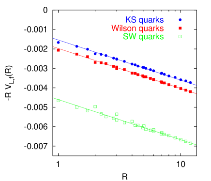
Figure 14: The same as Fig. 9 but for the fermionic contribution alone.

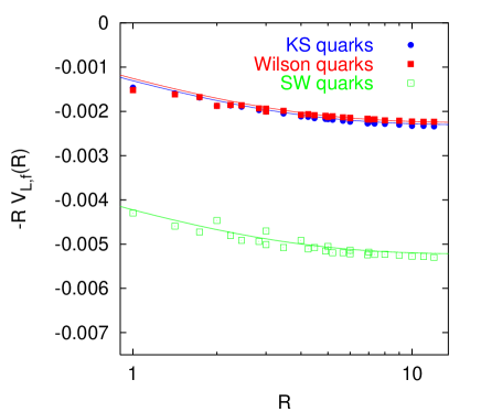
Figure 15: The same as Fig. 14 but for $ma=0.1$.

From Fig. 9 it is obvious that for realistic values of $n_{f}$ the potential is dominated by the gluonic contributions and the additional violations of rotational symmetry due to sea quarks that we have just discussed are an interesting but numerically subleading effect.

We shall now return to the limit where continuum perturbation theory is met, i.e. we investigate the behaviour at fixed (small) $a$ and large $r=Ra$. In the massless case this limit and the limit of large $R=r/a$ at fixed $r$ discussed above are equivalent, up to non-perturbative effects. However, as soon as a second scale $ma>0$ is introduced, the situation $r>m^{-1}$ becomes distinguishable from $r<m^{-1}$. In Fig. 14 we again display the self energy subtracted fermionic contribution $V_{L,f}({\mathbf{R}})$, this time multiplied by $-R$, in analogy to Fig. 9. This combination, multiplied by $C_{F}n_{f}$ isolates the shift that is induced onto an effective coupling $C_{F}\alpha_{R}$, due to sea quarks. The logarithmic slope of the three curves that are displayed in the figure is determined by the fermionic contribution to $\beta_{0}$ and is therefore universal. The inclusion of sea quarks not only reduces $\beta_{0}$, relative to the pure gauge case, and hence slows down the running of $\alpha_{R}$ but it also decreases the absolute value of the ${\mathcal{O}}(g^{4})$ coefficient. In the case of massive quarks, however, this effect is (over)compensated by an increase in the coupling $g^{2}$, relative to the pure gauge case, if we require the same physics at scales $r\gg m^{-1}$ where the sea quarks decouple. This will be discussed in Sec. IV.3.3 below.

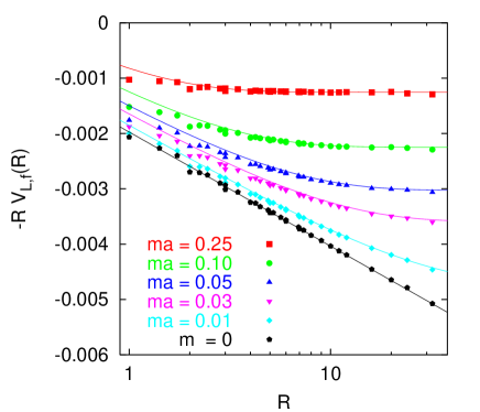
Figure 16: The same as Fig. 14 for Wilson fermions of various masses.

While for massless flavours the coupling runs logarithmically, for massive quarks the running gradually switches off around $R\approx 0.3/(ma)\approx 1/(\sqrt{C_{0}}ma)$: physics at length scales $Ra\gg m^{-1}$ is insensitive to the presence of massive sea quarks, at least in perturbation theory. In Fig. 15 we again compare the contributions to the effective Coulomb couplings resulting from the three different fermionic actions but for $ma=0.1$. At this mass value Wilson and KS results accidentally happen to be very close to each other. In Fig. 16 we investigate the mass dependence of the fermionic term somewhat more systematically by studying the example of Wilson quarks alone. In order to relate the lattice to a continuum scheme at large $R$, we not only have to subtract the (sea quark mass-dependent) static source self energy contribution to eliminate terms proportional to $R$ from the figure but also the vertical offset, $K_{1}(ma)$, at small $R$ changes due to a mass dependent term that appears in the conversion factor $b_{1}$ between the $\overline{MS}$ and the lattice scheme at finite $a$. We will discuss this effect in some detail in Sec. III.4 below.

In the limit $r\gg m^{-1}$ all curves indeed approach a constant value: the running of the effective coupling is not affected by the presence of massive sea quark flavours anymore. The resulting potential is the same as that in the pure gauge case, at least in perturbation theory, albeit with a different overall normalization of the effective Coulomb coupling. We shall discuss this shift of the QCD coupling constant at a given scale and the possibility of matching to the quenched theory in Sec. III.5 below.

While at large $R$ the lattice data and the continuum curve nicely coincide with each other [once the offset $K_{1}(ma)$ has been determined from the large $R$ data and subtracted], at small $R$ we observe large ${\mathcal{O}}(am)$ lattice artefacts, in addition to mass independent ${\mathcal{O}}(a)$ effects: even at the relatively small value $ma=0.03$ the lattice points lie systematically below the large $R$ expectation. Fig. 15 confirms this qualitative pattern for the other two fermionic actions.

III.4 “$\Delta K_{1}$”

As we have seen above the choice of lattice action not only affects the quality of rotational symmetry at small $R$ but also the overall normalization. The $\overline{MS}$ scheme is related to the lattice scheme via

$$\alpha_{\overline{MS}}(a^{-1})=\alpha_{L}+b_{1}\alpha^{2}+\cdots,$$ (40)

with the conversion factor

$$b_{1}=-\pi/(2N)+k_{1}N+K_{1}(ma)n_{f}.$$ (41)

The numerical constant $k_{1}$ is known for a variety of gluonic actions and $K_{1}(0)$ is known for Wilson, SW and KS quarks and independent of the gluonic action, cf. Eqs. (A.2) – (137).

The coefficients of the $\beta$-function in the $\overline{MS}$-scheme as well as in the lattice scheme in the continuum limit do not depend on the quark mass: both are “mass-independent” renormalization schemes. In lattice simulations it is often worthwhile to analyse quantities prior to an extrapolation to the continuum limit. One such example is determinations of the QCD running coupling from small Wilson loops El-Khadra:1992vn ; davi1 ; davi2 ; Spitz:1999tu ; Booth:2001qp ; davi3 that are ill-defined in this limit. We will discuss this technique in Sec. IV.2 below. Another example is simulations within the framework of an effective field theory like NRQCD Thacker:1991bm that requires a finite momentum cut-off.

At finite $a$ and $m>0$ the lattice scheme becomes mass-dependent, as indicated by the argument of the function,

$$K_{1}(ma)=K_{1}(0)+\Delta K_{1}(ma),$$ (42)

within Eq. (41). In this case universality is lost and the coefficients of the perturbative $\beta$-function acquire additional contributions that, like $\Delta K_{1}$, will in general depend on the dimensionful observable that is studied:

$$\beta_{0}^{\overline{MS}}-\beta_{0}^{L}=n_{f}\frac{d\Delta K_{1}(ma)}{d\ln a^{2}}.$$ (43)

By definition, $\Delta K_{1}(0)=0$. However, the behaviour of $\Delta K_{1}$ is also constrained in the limit $ma\rightarrow\infty$ where the sea quarks decouple and therefore $\beta_{0}^{\overline{MS}}=(11N)/(12\pi)$ while $\beta_{0}^{L}=\beta_{0}^{\overline{MS}}-n_{f}/(6\pi)$, i.e.,

$$\Delta K_{1}\stackrel{{\scriptstyle ma\rightarrow\infty}}{{\longrightarrow}}-\frac{1}{3\pi}\ln(Dma),$$ (44)

with a dimensionless constant $D$ that we calculate in Sec. III.5 below.

We have seen above that in the limit $r\ll m^{-1}$ the behaviour of the massless theory is emulated while the running of the potential for $r\gg m^{-1}$ is effectively quenched: the only scale that is relevant in perturbation theory in these limits is the distance $r$ (or, equivalently, momentum $q\approx r^{-1}$) and therefore lattice artefacts disappear like $(a/r)^{\nu}$ [or $(aq)^{\nu}$] with some positive integer power $\nu$, whose value depends on the lattice action, as $r\rightarrow\infty$. However, in the intermediate range of quark masses lattice corrections $(am)^{\nu}$ become relevant and the universality of the $\beta$-function is lost.

The function $K_{1}(ma)$ of Eq. (134) can in principle be read off from figures such as Figs. 15 and 16 up to short distance lattice artefacts: $K_{1}(ma)=-C_{F}/(4\pi)\,V_{L,2}(1)-\sqrt{C_{0}}ma+{\mathcal{O}}[(ma)^{2},a^{\nu}]$ [cf. Eqs. (III.2), (171) and (196)]. For the (improved) SW action not only the lattice artefacts are much more pronounced and qualitatively different from the Wilson and KS cases but also this overall offset $K_{1}$ is enhanced (although not its mass dependence).

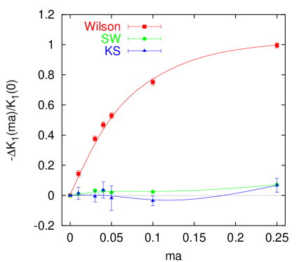
Figure 17: $\Delta K_{1}$ determined from the static position space potential, relative to $K_{1}(0)$.

Table 10: $\Delta K_{1}$ as a function of $ma$ for Wilson, SW and KS quarks. In the last row we display $-K_{1}(0)$ for comparison.

$ma$	$\Delta K_{1}^{(KS)}$	$\Delta K_{1}^{(W)}$	$\Delta K_{1}^{(SW)}$
0.01	0.0005(13)	0.0121(18)	0.0038(20)
0.03	-0.0002(12)	0.0316(15)	0.0131(19)
0.04	0.0012(18)	0.0394(18)	0.0127(20)
0.05	-0.0006(27)	0.0445(17)	0.0079(26)
0.10	-0.0012(11)	0.0632(17)	0.0095(10)
0.25	0.0023(15)	0.0837(14)	0.0280(14)
$-K_{1}(0)$	0.032983419	0.0841444	0.3957496

We determine $K_{1}(ma)$ from two parameter fits,

$$-\frac{4\pi R}{C_{F}}V_{L,2} = A_{0}+A_{1}\ln R+\frac{n_{f}}{3\pi}\mbox{Ein}\left(C_{0}^{1/2}maR\right)$$ (45)

$$+ n_{f}\Delta K_{1}(ma)+\frac{c}{R^{\nu}},$$

to the $R>9$ on-axis data points, with one redundant parameter $c$ whose role is to parametrize any residual lattice artefacts. The above functional form with the constants $A_{0}$ and $A_{1}$ of Eqs. (A.4) – (195) is motivated by Eq. (192) of Appendix A.4. The special function $\mbox{Ein}(x)$ denotes the normalized exponential integral defined in Eq. (172).

All fits turned out to be stable within statistical errors under variations of the fit range as well as consistent with the off-axis data. The results on $\Delta K_{1}$ are displayed in Tab. 10. In Fig. 17 these shifts are plotted relative to $-K_{1}(0)$, together with cubic splines. Since $K_{1}(0)<0$, at large $ma$ the curves will diverge towards the negative direction. Note that the slope of $\Delta K_{1}(ma)$ at $ma=0$ has also been determined in Ref. Booth:2001qp for SW fermions, however, by matching the vacuum polarization in momentum space, rather than the position space potential and $\Delta K_{1}$ is not universal.

For the two ${\mathcal{O}}(a)$ improved actions $\Delta K_{1}(ma)$ is small (a few %), relative to $K_{1}(0)$, at least for $ma\leq 1/4$. This is very different in the case of Wilson fermions, where even at $ma=0.05$ $\Delta K_{1}$ corrects $K_{1}(0)$ by more than 50 %. Using the static position space potential as the prescription that defines $\Delta K_{1}$, the $ma$ dependence is well parametrized by $\Delta K_{1}(x)=ax+bx^{2}$ with $a=1.20\pm 0.02$ and $b=-5.7\pm 0.3$ for $x=ma\leq 0.1$ in the Wilson case. For SW fermions the fit parameters read $a=0.44\pm 0.08$ and $b=-3.5\pm 0.8$ while the KS data are compatible with zero within our accuracy over the whole range $x\leq 0.25$ and can be fitted by a straight line with $a=-0.04\pm 0.04$.

III.5 The “$\beta$-shift”

We have seen above that at distances $r\gg m^{-1}$ the running of the coupling is not affected by the presence of sea quarks anymore: at large distances, at least in perturbation theory, the effect of massive quarks can be integrated out into a shift of the coupling constant of the quenched theory. In contrast this is not possible for a theory with massless quarks, which completely decouples from the quenched case at all scales.

The theory with massive sea quarks and the quenched theory can be matched in the infra red by use of an intermediate mass-dependent scheme, such as the $R$-scheme, defined through the inter-quark potential in position space,

$$\alpha_{R}\left(r^{-1}\right) = -\frac{r}{C_{F}}V_{c}(r)$$ (46)

$$\stackrel{{\scriptstyle R=r/a\rightarrow\infty}}{{\longrightarrow}} -\frac{Ra}{C_{F}}V_{\mbox{\scriptsize int}}(R)$$ (47)

Inserting the perturbative expansion of $V_{\mbox{\scriptsize int}}(R)$ in terms of $\alpha_{L}$ one obtains,

$$\alpha_{R}(\mu) = \alpha_{L}^{(n_{f})}+e_{1}^{(n_{f})}(R){\alpha_{L}^{(n_{f})}}^{2}+\cdots$$ (48)

$$= \alpha_{L}^{(0)}+e_{1}^{(0)}(R){\alpha_{L}^{(0)}}^{2}+\cdots,$$ (49)

where $\mu=(Ra)^{-1}$, with known coefficients, $e_{1}^{(n_{f})}(R)$. Note that these coefficients will depend on the function $K_{1}(ma)$ discussed above. The requirement of a unique (static source self-energy subtracted) potential $V_{\mbox{\scriptsize int}}(R)$ at $R\gg(ma)^{-1}$ then results in,

$$\alpha_{L}^{(0)}=\left\{1+\left[e_{1}^{(n_{f})}(\infty)-e_{1}^{(0)}(\infty)\right]\alpha\right\}\alpha_{L}^{(n_{f})}+\cdots.$$ (50)

One can now re-write the above equation in terms of the lattice parameter $\beta=2N/g^{2}=N/(2\pi\alpha_{L})$. For $n_{f}$ degenerate quark flavours with mass $m$ and $N=3$ the result reads,

$$\beta^{(n_{f})} = \beta^{(0)}+\Delta\beta,$$ (51)

$$\Delta\beta = \frac{n_{f}}{2\pi^{2}}\left[\ln(Dma)+3\pi\Delta K_{1}(ma)\right],$$ (52)

with the numerical values for the constant,

$$D=\sqrt{C_{0}}\exp\left[3\pi K_{1}(0)-\frac{5}{6}\right]:$$ (53)

$$D^{W} = 0.448\pm 0.002,$$ (54)

$$D^{SW} = 0.0238\pm 0.0001,$$ (55)

$$D^{KS} = 0.726\pm 0.002,$$ (56)

for Wilson, SW and KS fermions, respectively. Since $\Delta\beta\rightarrow 0$ as $ma\rightarrow\infty$, the $\ln(Dma)$ term has to be cancelled by $3\pi\Delta K_{1}(ma)$ at large $ma$ in Eq. (52): the constant $D$ is identical with that appearing within Eq. (44). We discuss the matching procedure in some more detail in Appendix B.

Naïvely one would assume perturbation theory to be applicable as long as the relative $\alpha$-shift is small. To leading non-trivial order in perturbation theory the $\beta$-shift is linear in $n_{f}$. At the next order, the situation will be complicated by additional terms that are proportional to $n_{f}^{2}$ as can be seen from Eq. (B.2) of Appendix B.

III.6 Boosted perturbation theory and $q^{*}$

Lattice perturbation theory is well known for its bad convergence, partly due to large contributions from lattice tadpole diagrams. We recall that $V_{2}({\mathbf{R}})$ incorporates such a contribution: $(2N^{2}-3)/(24N)V_{1}({\mathbf{R}})$ [cf. Eq. (III.1)]. Hence reordering the series in terms of a better behaved expansion parameter like $\alpha_{V}(q)$, the coupling defined by the static QCD potential in momentum space,

$$\tilde{V}(q)=-4\pi C_{F}\frac{\alpha_{V}(q)}{q^{2}},$$ (57)

is desirable in many cases. In some respect this is similar to the situation in continuum perturbation theory and resembles an expansion in terms of a renormalized, rather than a “bare”, lattice coupling parameter. We will refer to such techniques as “boosted perturbation theory”.

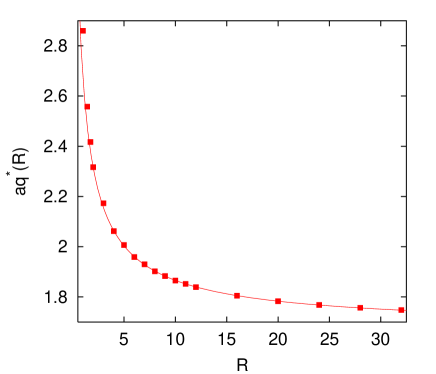
Figure 18: $q^{*}a$ values for the static potential.

At ${\mathcal{O}}(\alpha^{2})$ we can write,

$$\alpha_{V}(q^{*})=\alpha_{L}+\left[a_{1}+b_{1}-2\beta_{0}\ln(q^{*}a)\right]\alpha^{2},$$ (58)

with $a_{1}$, $b_{1}$ and $\beta_{0}$ as defined in Eqs. (154), (156), Eqs. (134) – (A.2) and Eq. (122), respectively. The “optimal” scale $q^{*}$ depends on the underlying process. It has been argued by Brodsky, Lepage and Mackenzie (BLM) Brodsky:1983gc ; lepage that the logarithmic average of the momenta exchanged at tree-level is a particularly good choice for the scale $q^{*}$ to be used within a one-loop calculation. The scale optimization procedure can also be generalized to higher order perturbative calculations Brodsky:1998mf ; Hornbostel:2002af . We illustrate the original recipe for the case of the position space potential. Here the tree-level calculation, Eq. (30), yields,

$$\ln\left[aq^{*}({\mathbf{R}})\right]=\frac{\int d^{3}\!q\ln q\sin^{2}\left(\frac{{\mathbf{q}}{\mathbf{R}}a}{2}\right)/\hat{\mathbf{q}}^{2}}{\int d^{3}\!q\sin^{2}\left(\frac{{\mathbf{q}}{\mathbf{R}}a}{2}\right)/\hat{\mathbf{q}}^{2}}.$$ (59)

For $R\gg 1$ we find,

$$aq^{*}(R)=f_{1}+\frac{f_{2}}{R}+f_{3}\frac{\ln R}{R}+\cdots,$$ (60)

with the numerical constants,

$$f_{1}\approx 1.672,f_{2}\approx 1.00,f_{3}\approx 0.41.$$ (61)

The constants $f_{2}$ and $f_{3}$ have been obtained from a fit to $R\geq 4$ data while the $r\rightarrow\infty$ limit $f_{1}$ has been calculated directly. The fit curve and $q^{*}$ values are displayed in Fig. 18. Note that violations of rotational invariance in $q^{*}({\mathbf{R}})$ are remarkably small. Analogously we can obtain $q^{*}$ values for the inter-quark force. We display results for the plaquette $\Box$, the chair, the “parallelogram”, the “rectangle” $W(1,2)$, the static self energy $\delta m_{\mbox{\scriptsize stat}}=V_{S}/2$, the potential and the force $F_{R_{1}R_{2}}=a[V(R_{2})-V(R_{1})]/(R_{2}-R_{1})$ at selected distances in Tab. 11. In addition, the $q^{*}$ values for the “tadpole improved” quantities $m_{\mbox{\scriptsize stat}}+\ln\Box/(4a)$ as well as $V(1)+\ln\Box/(2a)$ and $V(2)+\ln\Box/(2a)$ are included.

One can further convert between the $V$ and the $\overline{MS}$ scheme:

$$\alpha_{\overline{MS}}(\mu)=\alpha_{V}(q^{*})-\left[a_{1}+2\beta_{0}\ln(\mu/q^{*})\right]\alpha^{2}+\cdots.$$ (62)

It has been argued Brodsky:1983gc that the scale

$$\mu=e^{-5/6}q^{*},$$ (63)

at which the $n_{f}$ dependence of $a_{1}$ above is cancelled (in the massless case) was the optimal choice of scale for this conversion. Note that the ratio $\mu/q^{*}$ above is independent of the number of colours $N$ or flavours $n_{f}$. The $\mu$ values are also included into the table.

The average plaquette turns out to be the most ultra violet quantity, with $q^{*}\approx 3.402/a$, followed by the potential $V(R=1)$. Due to the self energy contribution $V_{S}=V(\infty)=2\delta m_{\mbox{\scriptsize stat}}$, $q^{*}$ is bounded from below by $1.672/a$ for the potential at all distances. However, in the case of the force $q^{*}_{F}\rightarrow 0$ as $R\rightarrow\infty$. As one would expect $q^{*}$ also approaches zero at large distances for the potential if $V_{S}$ is subtracted. We find for instance $q^{*}a\approx 0.59$ for $V(1)-V_{S}$ as opposed to $q^{*}a\approx 2.86$ for $V(1)$ alone.

Table 11: BLM scales $q^{*}$ for some quantities.

quantity	$q^{*}a$	$\mu a=e^{-5/6}q^{*}a$
$\Box$	3.402	1.478
chair	3.300	1.434
“parallelogram”	3.128	1.360
$W(1,2)$	3.066	1.332
$\delta m_{\mbox{\scriptsize stat}}$	1.672	0.727
$V(1)$	2.860	1.243
$V(2)$	2.317	1.007
$F_{12}$	1.025	0.445
$F_{23}$	0.904	0.393
$\delta m_{\mbox{\scriptsize stat}}+\ln\Box/(4a)$	0.835	0.363
$V(1)+\ln\Box/(2a)$	1.701	0.739
$V(2)+\ln\Box/(2a)$	1.316	0.572
$V(\sqrt{2})$	2.558	1.112
$V(\sqrt{3})$	2.417	1.050
$V(3)$	2.173	0.944
$V(4)$	2.062	0.896
$V(5)$	2.007	0.872
$V(6)$	1.959	0.851
$V(7)$	1.930	0.839
$V(8)$	1.902	0.826
$V(16)$	1.805	0.784
$V(24)$	1.768	0.768
$V(28)$	1.757	0.764
$V(32)$	1.748	0.760

III.7 The static source self energy

We define,

$$V_{S}=\lim_{R\to\infty}V(R)=2\delta m_{\mbox{\scriptsize stat}},$$ (64)

where $\delta m_{\mbox{\scriptsize stat}}$ is the lattice pole mass of a fundamental static colour source, e.g. a quark in the $m\rightarrow\infty$ limit. The above relation only holds in perturbation theory where the interaction energy vanishes as $r\rightarrow\infty$.

The static (or residual) mass $\delta m_{\mbox{\scriptsize stat}}$ has been calculated to ${\mathcal{O}}(\alpha^{3})$ for pure gauge theory DiRenzo:2001nd ; Trottier:2001vj as well as to ${\mathcal{O}}(\alpha^{2})$ for massless Wilson and SW quarks Martinelli:1999vt . This has enabled a number of authors to obtain the $b$ quark mass $\overline{m}_{b}(\overline{m_{b}})$ from lattice simulations of static-light mesons. Since the sources are static the ${\mathcal{O}}(\alpha)$ result can be obtained from a tree-level calculation and we count this as leading order (LO), discarding the trivial ${\mathcal{O}}(1)$ value $\delta m_{\mbox{\scriptsize stat}}=0$. The one-loop ${\mathcal{O}}(\alpha^{2})$ result is then next to leading order (NLO) and the two-loop ${\mathcal{O}}(\alpha^{3})$ value NNLO. Note that the counting conventions employed in some of the literature differ from the one defined above, in which ${\mathcal{O}}(\alpha^{n})$ corresponds to an N^mLO calculation with $m=n-1$ for which diagrams involving $m$ loops have to be computed. For instance in Ref. Martinelli:1999vt the value $m=n$ is used, creating the (wrong) impression that a two-loop calculation is required to obtain the ${\mathcal{O}}(\alpha^{2})$ result.

Table 12: Fermionic contributions to the static self energy of a fundamental source. The labelling conventions are defined in Eqs. (64) – (69).

$ma$	$\delta M_{f}^{(KS)}/10^{-3}$	$\delta M_{f}^{(0)}/10^{-3}$	$\delta M_{f}^{(1)}/10^{-3}$	$\delta M_{f}^{(2)}/10^{-3}$
0	-1.1667 (2)	-1.3404 (2)	0.1633 (5)	-1.8587 (6)
0.01	-1.500 (3)	-1.3061 (2)	0.1489 (1)	-1.8540(11)
0.03	-1.142 (3)	-1.2402 (2)	0.1216 (2)	-1.8443 (2)
0.04	-1.128 (2)	-1.2090 (1)	0.1083 (6)	-1.8397 (5)
0.05	-1.120 (3)	-1.1791 (1)	0.0967 (5)	-1.8364 (1)
0.10	-1.0801 (1)	-1.0447 (1)	0.0478 (1)	-1.8134 (1)
0.25	-0.922 (2)	-0.7541 (1)	-0.0268(1)	-1.7364 (1)
1	-0.2962 (1)	-0.2336 (2)	—	—
2	-0.06131(3)	-0.08264(6)	—	—
4	—	-0.02030(2)	—	—

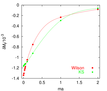
Figure 19: The fermionic contribution to the static self energy $\delta m_{\mbox{\tiny stat}}$ for Wilson and KS quarks as a function of the quark mass.

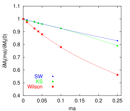
Figure 20: The fermionic contribution to the static self energy for Wilson, SW and KS quarks, normalized to the respective zero quark mass results.

We have computed the static quark mass shift as a function of the mass of three species of sea quarks: KS, Wilson and SW. The results, most of which can also be read off from the last seven lines of Tab. 9, are displayed in Tab. 12. The labelling conventions are identical to those of Eqs. (32) – (36):

$$a\delta m_{\mbox{\scriptsize stat}} = \delta M_{1}g^{2}+\delta M_{2}g^{4},$$ (65)

$$\delta M_{2} = \delta M_{pg}+C_{F}n_{f}\delta M_{f},$$ (66)

where

$$\delta M_{1} = \frac{C_{F}}{2}V_{1}(\infty),$$ (67)

$$\delta M_{pg} = \frac{C_{F}}{2}\left\{\frac{N}{2}\left[V_{\Pi}(\infty)+V_{NA}(\infty)\right]\right.$$ (68)

$$+ \left.\frac{2N^{2}-3}{24N}V_{T}(\infty)\right\}$$

and $\delta M_{f}=\delta M_{f}^{(KS)}$ for KS quarks and

$$\delta M_{f}=\delta M_{f}^{(0)}+c_{SW}\delta M_{f}^{(1)}+c_{SW}^{2}\delta M_{f}^{(2)}$$ (69)

for Wilson-SW fermions. We find the numerical values,

$$\delta M_{1} \approx 0.126365504\,C_{F}$$ (70)

$$\delta M_{pg} \approx 0.05292\,C_{F},$$ (71)

where the latter number applies to $SU(3)$ gauge theory (cf. the last line of Tab. 6). Note that this result differs in the least significant digit from the value obtained in Ref. Martinelli:1999vt that can be translated into $\delta M_{pg}\approx 0.05297C_{F}$. The mass dependence of $\delta M_{f}$ [which in Eq. (66) is accompanied by a factor $C_{F}n_{f}$] is visualized in Fig. 19 for Wilson and KS quarks. $\delta M_{f}$ approaches zero like $1/(ma)$ as $ma\rightarrow\infty$.

Finally, in Fig. 20 we compare the results on $\delta M_{f}(ma)$ for quark masses $ma\leq 0.25$, normalized to $\delta M_{f}(0)$, from all three quark actions with each other. While in absolute terms $\delta M_{f}$ for SW quarks turns out to be much bigger than for the other two actions (cf. Tab. 12) we find the relative variation with the quark mass to be much weaker for both ${\mathcal{O}}(a)$ improved actions than for Wilson fermions. This is consistent with our observations for small Wilson loops and $\Delta K_{1}$ above. For $ma\leq 0.1$ $\delta M_{f}(ma)$ is well parametrized by a quadratic function,

$$\delta M_{f}(ma)=\delta M_{f}(0)+b\,ma+c(ma)^{2},$$ (72)

with $\delta M_{f}(0)=-0.0011667(3),-0.0013404(2)$ and $-0.0030351(11)$, $b=0.00101(8)$, 0.00350(1) and 0.00245(5) and $c=-0.0014(8)$, $-0.00543(5)$ and $-0.0020(4)$ for KS, Wilson and SW quarks, respectively.

Table 13: Fermionic contributions to the static self energy as defined in Eqs. (74) – (78). The first three rows refer to the expansion of the tadpole improved observable in terms of $\alpha_{L}$, the last rows to an expansion in terms of $\alpha_{\overline{MS}}(0.363/a)$.

	KS	Wilson	SW
$a_{f}$	-0.1853	-0.2090	-0.5051
$b_{f}$	0.21	0.61	0.39
$c_{f}$	-0.38	-1.02	-0.33
$\overline{a}_{f}$	-0.03499	-0.05860	-0.3548
$\overline{b}_{f}$	0.26	-0.67	-0.081
$\overline{c}_{f}$	-0.38	5.08	3.41

Starting from the expansion of the plaquette,

$$\Box=1-c_{1}\alpha_{L}-c_{2}\alpha^{2}+\cdots,$$ (73)

we can rearrange the above expansion of the self energy in the following way,

$$a\delta m_{\mbox{\scriptsize stat}} = -\frac{\ln\Box}{4}+m_{1}^{t}\alpha_{L}+m_{2}^{t}\alpha_{L}^{2}$$ (74)

$$= -\frac{\ln\Box}{4}+m_{1}^{t}\alpha_{\overline{MS}}(\mu)+\overline{m}_{2}^{t}\alpha^{2},$$ (75)

where $\mu=q^{*}e^{-5/6}=0.363/a$, $m_{1}^{t}=(4\pi)\delta M_{1}-c_{1}/4$, $m_{2}^{t}=(4\pi)^{2}\delta M_{2}-c_{2}/4-c_{1}^{2}/8$. We will refer to practices such as adding the $\ln\Box$ term non-perturbatively and subtracting it perturbatively as “tadpole improvement” of the observable while in the second step, Eq. (75) we “boost” the perturbation theory. Here we choose to convert everything into the $\overline{MS}$ scheme. We prefer this to plaquette based schemes or the $V$ scheme as now all mass dependence is made explicit in the coefficient function $\overline{m}_{2}^{t}(ma)$. A conversion of the result into another scheme of choice including mass dependent schemes is easily possible with the help of Appendix A. We will obtain the $\overline{MS}$ coupling from the average plaquette and other quantities in Sec. IV.2 below.

For $SU(3)$ gauge theory with $n_{f}$ quark flavours of masses $ma\leq 0.1$ we find,

$$m_{1}^{t} = 1.0700768,$$ (76)

$$m_{2}^{t} = 7.6104+n_{f}\left[a_{f}+b_{f}ma+c_{f}(ma)^{2}\right],$$ (77)

$$\overline{m}_{2}^{t} = -0.5839+n_{f}\left[\overline{a}_{f}+\overline{b}_{f}ma+\overline{c}_{f}(ma)^{2}\right],$$ (78)

with the constants $a_{f}$, $b_{f}$, $c_{f},\ldots$ of Tab. 13. Tadpole improvement reduces the pure gauge value $\delta m_{pg}\approx 11.14$ to $m_{pg}^{t}\approx 7.61$ and boosting reduces this further down to $\overline{m}_{pg}^{t}\approx-0.584$. The fermionic coefficients $\delta m_{f}\mapsto a_{f}\mapsto\overline{a}_{f}$ also undergo a reduction in each step. The NNLO coefficient $\delta m_{3}\approx 86\mapsto m_{3}^{t}\approx 67.5\mapsto\overline{m}_{3}^{t}\approx 2.85$ is only known for $n_{f}=0$.

When applying the above result to extract say $m_{b}$ from lattice simulations in the static limit one can readily ignore the mass dependent terms for Wilson fermions, which are ${\mathcal{O}}(a)$ effects. However, it does not harm to include them either. In the cases of massive KS and SW sea quarks which are ${\mathcal{O}}(a)$ improved at least the $b_{f}$s have to be included.

IV Comparison with non-perturbative data

We shall compare and apply our perturbative calculations to non-perturbative results obtained in lattice simulations. For this purpose we will use several data sets that have been obtained by different collaborations. All quenched reference data are from simulations of one of the co-authors of this article and collaborators (Ref. Bali:2000gf and references therein) while $n_{f}=2$ data have been provided by the SESAM/T$\chi$L Collaboration Bali:2000vr ; Bali:2002 (Wilson fermions), the UKQCD Collaboration Allton:2001sk ; Booth:2001qp (SW fermions) and the MILC Collaboration Tamhankar:2000ce (KS fermions).

We will apply our perturbative results to the “$\beta$-shift” encountered when including sea quarks — relative to the quenched approximation. Subsequently we determine the QCD running coupling “constant” for $n_{f}=0$ and $n_{f}=2$ from lattice data of the correlation length Sommer:1994ce $R_{0}=r_{0}/a$, the average plaquette and the short distance static potential. In this context we will also make use of the CP-PACS Yoshie:2000wd ensemble obtained with $n_{f}=2$ SW fermions and the Iwasaki gluonic action Iwasaki:1984cj . Finally we shall also compare perturbative and non-perturbative lattice potentials with the aim of parametrizing lattice artefacts and to resolve the differences in the running of the Coulomb couplings between quenched and un-quenched data sets.

IV.1 The non-perturbative “$\beta$-shift”

We study the situation of $n_{f}$ mass-degenerate flavours of sea quarks. Two parameters can be varied: the coupling $\beta=6/g^{2}$ and the lattice quark mass $ma$ which in the case of Wilson-SW fermions is related to the parameter $\kappa$. Each $\kappa$-$\beta$ (or $ma$-$\beta$) combination can be translated into a pion mass $m_{\pi}r_{0}$ and a lattice spacing $a/r_{0}$ where $r_{0}$ is a correlation length defined below. As $\beta\rightarrow\infty$ we reach the continuum limit, $a/r_{0}\rightarrow 0$. Sending the quark mass $mr_{0}$ to zero corresponds to a vanishing pion mass, $m_{\pi}r_{0}\rightarrow 0$ (at finite $\beta$: only up to violations of chiral symmetry). However, in general the two limits will “mix”: varying $\beta$ at fixed $ma$ will not only affect $a/r_{0}$ but also to some extent the ratio $m_{\pi}r_{0}$ while a variation of $ma$, keeping the coupling fixed, will result in a change of $a/r_{0}$ as well.

In view of the computational cost of lattice simulations incorporating sea quarks, predicting by what amount the coupling has to be shifted in order to compensate for the change in $a/r_{0}$ that is induced by varying the quark mass $ma$ is certainly desirable. We will explore this possibility by comparing the expectation Eq. (52) on the perturbative $\beta$-shift against results from lattice simulations with $n_{f}=2$ sea quarks of masses $0.0098\leq ma\leq 0.3$.

At large distances the potentials will be dominated by non-perturbative effects: the quenched potential will linearly rise ad infinitum. However, as soon as sea quarks are introduced the $Z_{3}$ symmetry of the action is broken and at some distance Bali:2000vr $r_{c}\approx(2.10+1.56\,mr_{0})r_{0}$ string breaking will set in; obviously the linear quenched behaviour at large distances can never be emulated by a theory with a completely flat potential at large $r>r_{c}$. Sea quarks will also affect the running of the coupling at short distances $r<0.3\,m^{-1}$. Hence, the best we can hope for is that sea quarks decouple within a window of distances $m^{-1}\ll r<r_{c}$.

Table 14: Comparison between non-perturbative $\beta$-shifts $\Delta\beta_{r_{0}}$ and the respective perturbative predictions $\Delta\beta_{\mbox{\tiny 1-l}}$ for two flavours of Wilson fermions Bali:2000vr ; Bali:2002 .

$\beta$	$\kappa$	$ma$	$r_{0}/a$	$-\Delta\beta_{r_{0}}$	$-\Delta\beta_{\mbox{\tiny 1-l}}$
5.5	0.158	0.0597	4.03(3)	0.352(5)	0.318(3)
5.5	0.159	0.0398	4.39(3)	0.395(5)	0.371(4)
5.5	0.1596	0.0280	4.68(3)	0.427(4)	0.416(4)
5.5	0.160	0.0202	4.89(3)	0.450(4)	0.456(4)
5.6	0.156	0.0504	5.10(3)	0.373(5)	0.342(3)
5.6	0.1565	0.0402	5.28(5)	0.399(5)	0.369(4)
5.6	0.157	0.0300	5.46(5)	0.410(5)	0.406(4)
5.6	0.1575	0.0199	5.89(3)	0.454(5)	0.457(4)
5.6	0.158	0.0098	6.23(6)	0.488(7)	0.538(5)

Table 15: Comparison between non-perturbative $\beta$-shifts $\Delta\beta_{r_{0}}$ and the respective perturbative predictions $\Delta\beta_{\mbox{\tiny 1-l}}$ for two flavours of SW fermions Allton:2001sk ; Booth:2001qp .

$\beta$	$\kappa$	$ma$	$r_{0}/a$	$-\Delta\beta_{r_{0}}$	$-\Delta\beta_{\mbox{\tiny 1-l}}$
5.2	0.135	0.0459(2)	4.75(4)	0.736(5)	0.679(3)
5.2	0.1355	0.0236(2)	5.04(4)	0.766(5)	0.750(3)
5.2	0.13565	0.0179(9)	5.21(5)	0.784(6)	0.780(6)
5.25	0.1352	0.0427(2)	5.14(5)	0.723(6)	0.686(3)
5.26	0.1345	0.0720(2)	4.71(5)	0.671(5)	0.632(4)
5.29	0.134	0.0927(3)	4.81(5)	0.641(5)	0.609(3)
5.29	0.1350	0.0535(2)	5.26(7)	0.699(7)	0.664(3)
5.29	0.1355	0.0350(1)	5.62(9)	0.736(9)	0.708(3)

Table 16: Comparison between non-perturbative $\beta$-shifts $\Delta\beta_{r_{0}}$ and the respective perturbative predictions $\Delta\beta_{\mbox{\tiny 1-l}}$ for “two” flavours of KS fermions Tamhankar:2000ce . The $\beta=5.6$, $ma=0.025$ data point is from Ref. Heller:1994rz .

$\beta$	$ma$	$r_{0}/a$	$-\Delta\beta_{r_{0}}$	$-\Delta\beta_{\mbox{\tiny 1-l}}$
5.3	0.3	1.65(3)	0.079(25)	0.149(3)
5.35	0.3	1.79(1)	0.084(20)	0.149(3)
5.415	0.3	1.97(5)	0.076(9)	0.149(3)
5.3	0.2	1.75(5)	0.119(25)	0.196(2)
5.35	0.2	1.87(1)	0.111(13)	0.196(2)
5.415	0.2	2.15(1)	0.125(10)	0.196(2)
5.3	0.15	1.78(1)	0.130(20)	0.226(3)
5.35	0.15	1.94(1)	0.132(12)	0.226(3)
5.415	0.15	2.27(1)	0.154(11)	0.226(3)
5.3	0.1	1.86(2)	0.157(15)	0.267(2)
5.35	0.1	2.04(1)	0.161(10)	0.267(2)
5.415	0.1	2.45(1)	0.194(11)	0.267(2)
5.5	0.1	3.10(4)	0.225(7)	0.267(2)
5.3	0.075	1.91(2)	0.172(15)	0.295(2)
5.35	0.075	2.15(1)	0.190(10)	0.295(2)
5.3	0.05	1.96(2)	0.188(13)	0.336(2)
5.35	0.05	2.35(3)	0.237(13)	0.336(2)
5.415	0.05	2.72(1)	0.246(9)	0.336(2)
5.5	0.05	3.42(3)	0.273(6)	0.336(2)
5.3	0.025	2.03(1)	0.209(11)	0.406(1)
5.35	0.025	2.36(1)	0.240(12)	0.406(1)
5.415	0.025	2.95(1)	0.286(8)	0.406(1)
5.5	0.025	3.80(2)	0.324(5)	0.406(1)
5.6	0.025	4.8(1)	0.341(11)	0.406(1)
5.415	0.0125	3.12(2)	0.306(7)	0.476(1)
5.5	0.0125	3.98(1)	0.346(4)	0.476(1)
5.6	0.08	4.08(1)	0.259(4)	0.289(4)
5.6	0.04	4.54(2)	0.312(4)	0.358(1)
5.6	0.02	4.84(1)	0.345(3)	0.429(1)
5.6	0.01	4.99(1)	0.361(3)	0.499(1)

We shall define a

$$\Delta\beta_{r_{0}}(n_{f},r_{0}/a,ma)=\beta^{(n_{f})}(r_{0}/a,ma)-\beta^{(0)}(r_{0}/a),$$ (79)

by non-perturbatively matching un-quenched and quenched $\beta$ values that correspond to the same scale Sommer:1994ce $r_{0}\approx 0.5$ fm, implicitly defined through the relation,

$$\left.r_{0}^{2}\frac{dV(r)}{r}\right|_{r=r_{0}}=1.65.$$ (80)

If non-perturbative effects cancel from Eq. (79) and leading order perturbation theory applies then $\Delta\beta_{r_{0}}$ will only depend on $ma$ (and $n_{f}$) but not on the lattice spacing $a/r_{0}$. Perturbation theory will obviously break down for $ma\ll 1$ in which case the coefficients of the perturbative expansion explode [cf. Eq. (52)]. This is a reflection of the fact that the running of the coupling in the theory with massless sea quarks differs from the $n_{f}=0$ case at all scales.

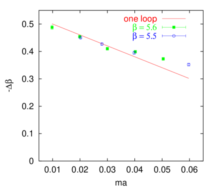
Figure 21: The non-perturbative $\beta$-shift for two flavours of Wilson fermions, in comparison with the perturbative prediction (curve).

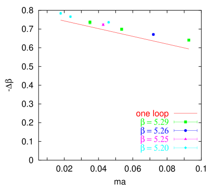
Figure 22: The non-perturbative $\beta$-shift for two flavours of SW fermions.

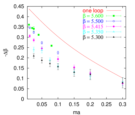
Figure 23: The non-perturbative $\beta$-shift for “two” flavours of KS fermions.

On the other hand, unless $ma\ll 1/D$ the relative importance of the non-universal term $\Delta K_{1}(ma)$ will increase and in general the matching of the running of the inter-quark force at a scale $r_{0}$ is not equivalent to the matching of the running of the potential at larger distances anymore. In principle one can work out the matching condition for $r_{0}$ in perturbation theory. It turns out, however, that at distances $r_{0}\approx 0.5$ fm the non-perturbative contribution to the lattice potential is already substantial. For instance a perturbative $n_{f}=0$ calculation yields $r_{0}/a=5.33$ at $\beta\approx 1.49$ while non-perturbatively this result is obtained at $\beta\approx 6.0$ and $\beta$ depends only logarithmically on $a$!

Given the above situation, it is difficult to identify a sensible way of combining perturbative and non-perturbative results at large distances. Consequently, we refrain from attempting to do this but separately employ purely perturbative and purely non-perturbative matching strategies: on the lattice simulation side of things we match $r_{0}/a$. In perturbation theory we match a quantity that is suitable for perturbative treatment, namely the inter-quark potential at large distances, rather than a quantity that is inspired by (non-perturbative) phenomenology, like $r_{0}$. We then hope that some, ideally most, non-perturbative effects cancel each other on the right hand side of Eq. (79) and leave the $\beta$-shift within the available window of $r_{0}/a$ and $ma$ untouched. Clearly, the perturbative matching will break down if either $ma$ or $\beta$ are too small. In addition the strategy that we adopt requires $ma<1/D$ to limit violations of universality as well as $mr_{0}>0.3$ to ensure that the sea quarks do not affect the running of the coupling at distances around $r_{0}$.

The quenched $\beta$ value that corresponds to a given $r_{0}/a$ is determined by use of the interpolation,

$$r_{0}/a=\exp\left(d_{0}+d_{1}x+d_{2}x^{2}+d_{3}x^{3}\right),\quad x=\beta-5.9,$$ (81)

with $d_{0}\approx 1.489,d_{1}\approx 1.982,d_{2}\approx-0.630,d_{3}\approx-1.522$, obtained from a fit to lattice results within the window Bali:2000gf $5.5\leq\beta\leq 6.2$. In principle we can also use the more recent precision data of Refs. Guagnelli:1998ud ; Necco:2002xg . However, the difference is insignificant in view of the present level of accuracy of un-quenched data and the matching of some of the MILC data requires an interpolation that extends to lattice spacings coarser than those investigated in the latter two references. In the un-quenched simulations, different groups used different procedures to extract $r_{0}/a$ which partly explains why different collaborations can obtain very different error estimates with similar computational efforts. Aiming only at a qualitative comparison we shall not attempt to reanalyse all data in one and the same way but prefer to cite the published values and errors.

In the case of KS fermions Tamhankar:2000ce ; Heller:1994rz there is no additive mass renormalization. For Wilson fermions Bali:2000vr ; Bali:2002 we define the lattice quark mass via,

$$ma=\frac{1}{2}\left(\frac{1}{\kappa}-\frac{1}{\kappa_{c}}\right),$$ (82)

where $\kappa_{c}$ has been obtained from a chiral extrapolation of the non-perturbative $m_{\pi}^{2}$ at fixed $\beta$. In the case of the SW data Allton:2001sk ; Booth:2001qp we do not know $\kappa_{c}$ but we can use the published values of the PCAC quark mass Allton:2001sk , which is equivalent to any other definition to leading order perturbation theory.

We compile results from the three collaborations in Tabs. 14 – 16. We have sorted Tab. 16 (with the exception of $\beta=5.6$) with respect to the quark mass and then $\beta$ while the other tables are sorted the other way around. Unfortunately, no PCAC mass value is available for the most critical UKQCD data set [$(\beta,\kappa)=(5.2,0.13565)$], however, we arrived at the estimate $ma=0.0179(9)$ by extrapolating $ma$ as a linear function of $(m_{\pi}r_{0})^{2}$ to the value Hepburn:2002fh $(m_{\pi}r_{0})^{2}=0.132(2)$. The perturbative prediction Eq. (52) is included in the last column of the tables where the error is due to the uncertainty in $\Delta K_{1}(ma)$.

In Figs. 21 – 23 we compare the non-perturbative results with the expectations. In all cases $ma$ is much smaller than $1/D$ as desired. However, $mr_{0}$, varying from 0.06 to 0.24 in the Wilson case, from 0.09 to 0.46 in the SW case and from 0.04 to 0.6 in the KS case, is not exactly big relative to $r_{0}=0.3\,m^{-1}$ (the distance below which the perturbative running of the coupling changes and sea quark effects cannot completely be compensated for by a scale redefinition alone). Nonetheless, the first two figures reveal an excellent agreement with the expectation within 10 % for Wilson-type quarks, even for such light quark masses. Moreover, no significant $\beta$-dependence is observed, again in agreement with Eq. (52), indicating higher order corrections to be small. This is very different for the KS fermions depicted in Fig. 23: here the agreement with the prediction only improves as the lattice spacing is reduced.

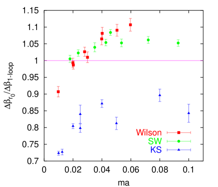
Figure 24: $\beta$-shift: the non-perturbative result, normalized to the prediction.

In Fig. 24 we finally compare the three formulations within the window $0.1\geq ma\geq 0.009$ for $4<r_{0}/a<6.5$ data. The Wilson and SW results seem to fall onto almost universal curves that differ by less than 10 % from the prediction while the KS results deviate by much more and some $\beta$-dependence is evident, Whether this is due to a slower convergence of the perturbative series, due to the inexact updating algorithm employed or due to $n_{f}$ not being a multiple of four is an open question. Around $m\approx 0.05\,r_{0}^{-1}\approx 20$ MeV the reliability of the matching for Wilson-SW quarks finally appears to break down (left-most data point in Fig. 24): the behaviour becomes “truly un-quenched”.

We remind the reader that $\beta$-shifts are in general not independent of the quantity that is used to match quenched and un-quenched theories. This ambiguity exists non-perturbatively as well as in perturbation theory. The qualitative agreement between prediction and simulation for Wilson-type quarks indicates that, at least at present masses, physics at hadronic scales is not yet strongly affected by quark loops, which is consistent with the phenomenological success of the quenched approximation.

In simulations with non-perturbatively improved SW quarks the lines of constant $a/r_{0}$ and constant $m_{\pi}r_{0}$ are significantly tilted with respect to both axes of the $\beta$-$ma$ plane Irving:2001hs . This observation is consistent with the small value, $D^{SW}\approx 0.0238$, but causes practical problems as going to lighter quark masses at sensible $a/r_{0}$ values requires simulations at small $\beta$s for which the non-perturbative determination of the improvement coefficient $c_{SW}$ causes problems Jansen:1998mx . In the worst case it might even be conceivable that the slope of the variation of $a/r_{0}$ with $\kappa\rightarrow\kappa_{c}$ at fixed $\beta$ eventually diverges and that the continuum limit $\beta\rightarrow\infty$ does not at all exist for light quarks Aoki:1983qi ; Aoki:2001xq . The variation of $r_{0}$ with the quark mass, however, is reduced when actions with only moderately negative values of $K_{1}(0)$ [and therefore $D$ values that are of order one] like the Wilson or KS action are employed.

Our result might be taken as an indication that the perturbative matching of $n_{f}-1$ to $n_{f}$ QCD couplings in the $\overline{MS}$ scheme via the intermediate mass-dependent $V$-scheme Brodsky:1998mf (or by calculating and matching a physical amplitude Bernreuther:1983zp ) is likely to be quite reliable, even at masses as light as or lighter than that of the charm quark. In this case the matching condition reads,

$$\frac{1}{\alpha^{(n_{f})}_{\overline{MS}}(\mu)}=\frac{1}{\alpha^{(n_{f}-1)}_{\overline{MS}}(\mu)}+\frac{1}{3\pi}\left[\ln\left(\sqrt{C_{0}}\frac{m}{\mu}\right)-\frac{5}{6}\right]\alpha,$$ (83)

which may be rewritten as,

$$\alpha^{(n_{f})}_{\overline{MS}}(\mu)=\alpha^{(n_{f}-1)}_{\overline{MS}}(\mu),$$ (84)

where,

$$\mu=\sqrt{C_{0}}\exp\left(-\frac{5}{6}\right)m=0.990(3)m,$$ (85)

to this order in perturbation theory. Clearly, the applicability of the matching method in this case is ultimately limited by the reliability of the perturbative running of the $\overline{MS}$ coupling at small scales.

IV.2 Determining $\alpha_{\overline{MS}}$

Lattice simulations yield correlation lengths and masses that are functions of a set of input parameters, namely the inverse lattice coupling $\beta$ and lattice quark masses $ma$ (or in the case of Wilson-type fermions $\kappa$-values that can be related to the quark masses). One can then for instance obtain the strong coupling constant in the $\overline{MS}$ scheme,

$$\alpha_{\overline{MS}}(a^{-1})=\alpha_{L}+b_{1}\alpha_{L}^{2}+\cdots,$$ (86)

once a physical scale has been assigned to the lattice spacing $a$. One such possibility would be to “measure” $R_{0}=r_{0}/a$ on the lattice and to equate $r_{0}\approx 0.5$ fm. Other input scales with a more direct connection to experiment are possible, for instance the proton mass $m_{N}$ or the pion decay constant $f_{\pi}$. If QCD with the right number of quark flavours and masses is simulated the resulting $a$ should become independent of the choice of the experimental input quantity. In this way the strong coupling constant can be determined from low energy hadron phenomenology.

There are of course higher order perturbative as well as non-perturbative corrections to Eq. (86) which, however, will vanish as $a\rightarrow 0$. In practice these corrections are big in the range of lattice spacings that will ever be realistically accessible Bali:1993ru ; lepage . One way to improve the convergence is to convert between the $\overline{MS}$ and the lattice schemes at an optimized BLM scale Brodsky:1983gc ; lepage ; Brodsky:1998mf $\mu=e^{-5/6}q^{*}$, rather than at $a^{-1}$. We refer to this reorganization of the perturbative series as boosted perturbation theory. Another possibility (that can be combined with the BLM scheme) is to “measure” the coupling on the lattice. This can either be done from a quantity that depends on the lattice spacing like the average plaquette Parisi:1980pe ; lepage ; El-Khadra:1992vn ; davi1 ; davi2 or at a scale $\mu\ll a^{-1}$ from quantities that have a well defined continuum limit Booth:1992bm ; Bali:1993ru ; Necco:2001gh ; Garden:2000fg . Here we shall follow the former strategy.

Table 17: Pure gauge $SU(3)$ results on $r_{0}$ and the average plaquette $\Box$.

$\beta$	$r_{0}/a$	$\Box$
5.5	2.01(3)	0.49680(2)
5.6	2.44(6)	0.52451(3)
5.7	2.86(5)	0.54919(3)
5.8	3.64(5)	0.56765(2)
5.9	4.60(9)	0.58184(2)
6.0	5.33(3)	0.59368(1)
6.2	7.29(4)	0.61363(1)
6.3	8.39(7)	0.62243(1)
6.4	9.89(16)	0.63064(1)
6.6	12.73(14)	0.64567(1)

Table 18: Pure gauge $SU(3)$ results on the short distance potential and force $F_{R_{1}R_{2}}=a[V(R_{2})-V(R_{1})]$.

$\beta$	$aV(1)$	$aV(2)$	$F_{12}$	$F_{23}$
5.5	0.636 (2)	1.155(21)	0.519(22)	0.29 (17)
5.6	0.566 (1)	0.963 (4)	0.398 (5)	0.325(16)
5.7	0.506 (2)	0.804 (5)	0.297 (5)	0.233(15)
5.8	0.464 (1)	0.706 (3)	0.242 (3)	0.160 (6)
5.9	0.4330(9)	0.645 (2)	0.212 (2)	0.127 (4)
6.0	0.4111(2)	0.5974(2)	0.1863(2)	0.1032(4)
6.2	0.3778(1)	0.5337(1)	0.1559(1)	0.0783(2)
6.4	0.3514(2)	0.4889(4)	0.1375(4)	0.0648(5)
6.6	0.3293(2)	0.4538(3)	0.1244(3)	0.0546(5)

Table 19: Average plaquette, short range potential and force with two flavours of Wilson quarks. The corresponding $r_{0}/a$ and $ma$ values can be found in Tab. 14.

$\beta$	$\kappa$	$\Box$	$aV(1)$	$aV(2)$	$F_{12}$
5.5	0.158	0.55547(4)	0.4756(3)	0.7156(10)	0.2400(10)
5.5	0.159	0.55815(3)	0.4685(3)	0.6965 (9)	0.2280 (9)
5.5	0.1596	0.55967(3)	0.4644(2)	0.6853 (7)	0.2209 (7)
5.5	0.160	0.56077(5)	0.4616(3)	0.6761 (8)	0.2145 (8)
5.6	0.156	0.56989(1)	0.4460(2)	0.6511 (6)	0.2051 (6)
5.6	0.1565	0.57073(1)	0.4440(3)	0.6450 (9)	0.2010 (9)
5.6	0.157	0.57160(1)	0.4422(3)	0.6387(11)	0.1965(10)
5.6	0.1575	0.57257(1)	0.4394(2)	0.6336 (6)	0.1942 (6)
5.6	0.158	0.57337(1)	0.4373(3)	0.6303(13)	0.1930(12)

IV.2.1 The method

We collect the average plaquette, the potential at $R=1$ and at $R=2$ obtained in quenched simulations as well as from simulations with sea quarks in Tabs. 17 – 21. In addition we include the “force”,

$$F_{12} = a\left[V(2)-V(1)\right],$$ (87)

$$F_{23} = a\left[V(3)-V(2)\right].$$ (88)

We will restrict our discussion to a one-loop determination of the running coupling. We shall also calculate two-loop corrections for the pure gauge case. Two-loop results are also known for the case of the plaquette with massive Wilson quarks Alles:1998is .

Table 20: The same as Tab. 19 but with two flavours of SW quarks. The corresponding $r_{0}/a$ and $ma$ values can be found in Tab. 15.

$\beta$	$\kappa$	$\Box$	$aV(1)$	$aV(2)$	$F_{12}$
5.2	0.135	0.53368(1)	0.4823(2)	0.6970 (8)	0.2147 (8)
5.2	0.1355	0.53629(1)	0.4762(2)	0.6832 (8)	0.2070 (8)
5.2	0.13565	—	0.4749(2)	0.6794 (6)	0.2045 (6)
5.25	0.1352	0.54113(2)	—	—	—
5.26	0.1345	0.53973(1)	0.4739(4)	0.6839(11)	0.2100(11)
5.29	0.134	0.54241(1)	0.4707(3)	0.6782(10)	0.2075(10)
5.29	0.1350	0.54552(3)	—	—	—
5.29	0.1355	0.54708(3)	—	—	—

Table 21: The same as Tab. 19 but with “two” flavours of KS quarks. The corresponding $r_{0}/a$ values can be found in Tab. 16.

$\beta$	$ma$	$\Box$	$aV(1)$	$aV(2)$	$F_{12}$
5.3	0.3	0.46980(6)	0.7055(35)	1.35 (14)	0.64 (14)
5.3	0.2	0.47554(8)	0.6848(34)	1.114 (9)	0.429 (9)
5.3	0.15	0.4792 (4)	0.6740(17)	1.299 (6)	0.625 (6)
5.3	0.1	0.48444(8)	0.6534(24)	1.291 (8)	0.638 (8)
5.3	0.075	0.48714(8)	0.6512 (4)	1.1580(18)	0.5068(18)
5.3	0.05	0.48918(9)	0.6419(14)	1.135 (35)	0.493 (35)
5.3	0.025	0.49238(8)	0.6301(10)	1.096 (20)	0.466 (20)
5.35	0.3	0.48243(5)	0.6724(14)	1.258 (6)	0.586 (6)
5.35	0.2	0.48912(5)	0.6482(13)	1.163 (36)	0.515 (36)
5.35	0.15	0.49373(5)	—	—	—
5.35	0.1	0.49951(4)	0.6154(10)	1.024 (18)	0.409 (18)
5.35	0.075	0.50283(5)	0.6066(10)	1.032 (18)	0.425 (18)
5.35	0.05	0.50565(6)	0.5980 (9)	1.014 (13)	0.416 (13)
5.35	0.025	0.51097(6)	0.5822 (8)	0.976 (10)	0.394 (10)
5.415	0.3	0.50065(6)	0.6223(15)	1.113 (37)	0.491 (37)
5.415	0.2	0.50841(8)	0.5980(14)	1.009 (15)	0.411 (15)
5.415	0.15	0.51366(6)	0.5834 (8)	0.977 (13)	0.394 (13)
5.415	0.1	0.52007(7)	0.5627 (9)	0.948 (8)	0.385 (8)
5.415	0.05	0.52692(5)	0.5422 (5)	0.8711(42)	0.3289(42)
5.415	0.025	0.53066(4)	0.5295 (5)	0.8449(35)	0.3154(35)
5.415	0.0125	0.5329 (1)	0.5222 (5)	0.8231(35)	0.3009(35)
5.5	0.1	0.54328(2)	0.5070 (3)	0.8001(17)	0.2931(17)
5.5	0.05	0.54724(2)	0.4935 (1)	0.7592 (5)	0.2657 (5)
5.5	0.025	0.54932(2)	0.4862 (2)	0.7375(11)	0.2513(11)
5.5	0.0125	0.55027(2)	0.4829 (2)	0.7289(11)	0.2460(11)
5.6	0.08	0.56325(2)	0.4616 (1)	0.6904 (7)	0.2288 (7)
5.6	0.04	0.56418(1)	0.4566 (1)	0.6763 (5)	0.2197 (5)
5.6	0.02	0.56479(1)	0.4537 (1)	0.6670 (7)	0.2133 (7)
5.6	0.01	0.56499(1)	0.4528 (1)	0.6619 (6)	0.2091 (6)

Obviously many ways, some better than others, to extract $\alpha_{\overline{MS}}$ exist that are consistent with perturbation theory at a given order. For convenience we adopt the procedure detailed in Refs. davi1 ; davi2 but point out that many alternative ways are equally justified (e.g. that of Ref. Booth:2001qp ). We only differ from Refs. davi1 ; davi2 in as far as, once the coupling has been converted into the $\overline{MS}$ scheme, we evolve the scale and extract the $\Lambda$-parameter by numerically integrating the four-loop $\beta$ function, rather than using a perturbatively truncated formula.

We can write the plaquette as,

$$\Box=1-c_{1}\alpha_{L}-c_{2}\alpha_{L}^{2}-c_{3}\alpha_{L}^{3},$$ (89)

where $c_{1}$ and $c_{2}$ can be read off from Tab. 1 with the help of Eqs. (19) – (22) for the pure gauge case and the fermionic contributions can be identified in Tabs. 4 and 5. In particular one finds $c_{1}=4\pi C_{F}/4$. $c_{3}$ for the pure gauge case and sources in the fundamental representation reads Alles:1994dn ; Alles:1998is :

$$c_{3}\approx \frac{(N^{2}-1)N}{8}\left[0.0063538-\frac{0.0181239}{N^{2}}\right.$$ (90)

$$\left.+\frac{0.0185221}{N^{4}}\right](4\pi)^{3}.$$

We now define the quantity,

$$P = -\frac{\ln\Box}{c_{1}}$$ (91)

$$= \alpha_{L}+\tilde{c}_{1}\alpha_{L}^{2}+\tilde{c}_{2}\alpha_{L}^{3},$$ (92)

$$\tilde{c}_{1} = \frac{c_{2}}{c_{1}}+\frac{c_{1}}{2},$$ (93)

$$\tilde{c}_{2} = \frac{c_{3}}{c_{1}}+c_{2}+\frac{c_{1}^{2}}{3}.$$ (94)

The expansion of $P$ in terms of $\alpha_{L}$ suffers from big coefficients. For instance one obtains $\tilde{c}_{1}\approx 3.37$, $\tilde{c}_{2}\approx 17.69$ in $SU(3)$ pure gauge theory. The origin of these big numbers can be traced to the lattice tadpole diagrams lepage . Large coefficients are also encountered when $\alpha_{L}$ is converted into the more “physical” coupling $\alpha_{V}$ [or $\alpha_{\overline{MS}}$ which is “close” to $\alpha_{V}$, cf. Eq. (175)]. By re-expressing the series Eq. (92) in terms of $\alpha_{V}$, taken at a suitable scale $q^{*}$ Brodsky:1983gc , one might hope that the two effects cancel in part lepage :

$$P=\alpha_{V}(q^{*})+X_{1}(q^{*}a)\alpha_{V}^{2}(q^{*})+X_{2}(q^{*}a)\alpha_{V}^{3}+\cdots.$$ (95)

We obtain,

$$X_{1}(x) = \tilde{c}_{1}+B_{1}(x)$$ (96)

$$X_{2}(x) = \tilde{c}_{2}+B_{2}(x)+2\tilde{c}_{1}B_{1}(x),$$ (97)

where

$$B_{1}(x) = -b_{1}-a_{1}+2\beta_{0}\ln x$$ (98)

$$B_{2}(x) = -b_{2}-a_{2}+2(a_{1}b_{1}+b_{1}^{2}+a_{1}^{2})$$ (99)

$$+ 2\beta_{1}\ln x+B_{1}^{2}(x)-B_{1}^{2}(1).$$

The constant $b_{1}$ is defined in Eqs. (134) – (137), $b_{2}$ in Eqs. (140) – (A.2) and $\beta_{i}$ in Eqs. (122) – (123). The $a_{i}$ are defined in Eqs. (154) and (A.3) and have to be taken at the scale $q^{*}$ for massive sea quarks. The numerical values for $n_{f}=0$ and $q^{*}a\approx 3.402$ read: $X_{1}\approx-1.191$, $X_{2}\approx-1.688$. We can now truncate Eq. (95) at ${\mathcal{O}}(\alpha^{2})$ and obtain,

$$\alpha_{V}(q^{*}) = \alpha_{P}-X_{2}\alpha_{P}^{3}+\cdots,$$ (100)

$$\alpha_{P} = \frac{1}{2X_{1}}\left(\sqrt{4PX_{1}+1}-1\right).$$ (101)

Note that the coefficients $X_{i}$ inherit a mass dependence from $a_{i}$, $b_{i}$ (through $\Delta K_{i}$) and $\tilde{c}_{i}$. With

$$\alpha_{\overline{MS}}(\mu) = \alpha_{V}(q^{*})+Y_{1}\alpha_{V}^{2}(q^{*})+Z_{2}\alpha_{V}^{3}(q^{*}),$$ (102)

$$\mu = e^{-5/6}q^{*}\approx 1.478/a,$$ (103)

$$Y_{1} = -\left(a_{1}-\frac{5}{3}\beta_{0}\right),$$ (104)

$$Z_{2} = -\left[a_{2}-a_{1}^{2}-\frac{5}{3}\beta_{1}-\left(a_{1}-\frac{5}{3}\beta_{0}\right)^{2}\right],$$ (105)

we arrive at,

$$\alpha_{\overline{MS}}(\mu)=\alpha_{P}+Y_{1}\alpha_{P}^{2}+Y_{2}\alpha_{P}^{3},$$ (106)

where

$$Y_{1} = \frac{2N}{3\pi}-\frac{n_{f}}{6\pi}\ln\left(1+\frac{C_{0}m^{2}}{{\mu}^{2}}\right),$$ (107)

$$Y_{2} = Z_{2}-X_{2}.$$ (108)

For $m=0$ $Y_{1}$ is independent of $n_{f}$. For $n_{f}=0$, $N=3$ we find the numerical value, $Y_{2}\approx 0.9538$: the NNLO correction is small.

In analogy to defining a coupling from the measured plaquette, other couplings can be computed from force and potential. We illustrate this procedure at NLO: in a first step we can write,

$$\frac{aV({\mathbf{R}}a)}{v_{1}({\mathbf{R}})} = \alpha_{L}+\frac{v_{2}({\mathbf{R}})}{v_{1}({\mathbf{R}})}\alpha^{2}$$ (109)

$$= \alpha_{V}(q^{*})+\left[\frac{v_{2}({\mathbf{R}})}{v_{1}({\mathbf{R}})}+B_{1}(q^{*}a)\right]\alpha^{2},$$

where the function $B_{1}(x)$ is defined in Eq. (98). A similar expression can easily be written down for the force. The respective $q^{*}a$ values can be found in Tab. 11. Consequently, $\alpha_{V}(q^{*})$ can be obtained by solving the quadratic equation Eq. (109) and converted into $\alpha_{\overline{MS}}(\mu)$ via Eqs. (106) and (107), where we set $Y_{2}=0$ in our ${\mathcal{O}}(\alpha^{2})$ calculation.

Finally, we can run $\alpha_{\overline{MS}}$ numerically to arbitrarily high scales using the perturbative four-loop $\beta$ function vanRitbergen:1997va ; Tarasov:1980au and then determine the $\Lambda_{\overline{MS}}$-parameter, defined as in Eq. (125).

IV.2.2 Pure gauge theory

We display one- and two-loop results on $\alpha_{\overline{MS}}(\mu)$ as obtained from the logarithm of the average plaquette following the boosted perturbation theory procedure detailed above (as well as in Refs. davi1 ; davi2 ), in Tab. 22. This is then numerically converted into estimates of the QCD $\Lambda_{\overline{MS}}$-parameter which are displayed in the last two columns of the table. In Fig. 25 we compare various methods of determining the $\overline{MS}$ $\Lambda$-parameter as a function of the lattice spacing. The horizontal error band corresponds to the continuum limit result as obtained by the ALPHA Collaboration Garden:2000fg by use of finite volume techniques. $\alpha_{L}$ refers to a conversion from the bare lattice coupling $\alpha_{L}=3/[2\pi\beta(a)]$ and $\alpha_{P}$ to a coupling, “measured” from the average plaquette. NLO and NNLO refer to results from a naïve perturbative conversion of $\alpha_{L}$ into $\alpha_{\overline{MS}}(a^{-1})$ at order $\alpha^{2}$ and $\alpha^{3}$ respectively while the abbreviations bNLO and bNNLO correspond to the boosted perturbation theory procedure detailed above.

Table 22: $\mu=e^{-5/6}q^{*}$ in $SU(3)$ pure gauge theory and one- (1-l) and two-loop (2-l) estimates of $\alpha_{\overline{MS}}(\mu)$ and $\Lambda_{\overline{MS}}$ from the average plaquette. The errors of $\alpha$ do not reflect the uncertainty in the scale $\mu$.

$\beta$	$\mu r_{0}$	$\alpha_{\overline{MS},\mbox{\tiny 1-l}}$	$\alpha_{\overline{MS},\mbox{\tiny 2-l}}$	$\Lambda_{\overline{MS},\mbox{\tiny 1-l}}r_{0}$	$\Lambda_{\overline{MS},\mbox{\tiny 2-l}}r_{0}$
5.5	2.97 (4)	0.26368(3)	0.27517(3)	0.604 (9)	0.648 (9)
5.6	3.61 (9)	0.22947(3)	0.23747(3)	0.568(15)	0.608(15)
5.7	4.23 (7)	0.20417(3)	0.21000(3)	0.517 (9)	0.551 (9)
5.8	5.38 (7)	0.18753(2)	0.19216(2)	0.532 (7)	0.566 (7)
5.9	6.80(13)	0.17582(2)	0.17970(2)	0.566(12)	0.601(12)
6.0	7.88 (4)	0.16667(1)	0.17000(1)	0.562 (3)	0.596 (3)
6.2	10.78 (6)	0.15233(1)	0.15494(1)	0.580 (3)	0.613 (3)
6.3	12.40(10)	0.14639(1)	0.14873(1)	0.584 (5)	0.616 (5)
6.4	14.62(24)	0.14105(1)	0.14316(1)	0.603(10)	0.636(10)
6.6	18.82(21)	0.13172(1)	0.13346(1)	0.601 (7)	0.632 (7)

Table 23: Boosted NLO pure gauge estimates of $\alpha_{\overline{MS}}(\mu)$ from $aV(1)$, $aV(2)$, $F_{12}$ and $F_{23}$, respectively. The respective scales $\mu r_{0}$ can easily be read off from Tabs. 11 and 17. The errors of $\alpha$ do not reflect the uncertainty in $\mu r_{0}$.

$\beta$	$\alpha_{\overline{MS}}^{V_{1}}(\mu)$	$\alpha_{\overline{MS}}^{V_{2}}(\mu)$	$\alpha_{\overline{MS}}^{F_{12}}(\mu)$	$\alpha_{\overline{MS}}^{F_{23}}(\mu)$
5.5	0.3414(17)	0.629(27)	—	—
5.6	0.2862 (7)	0.4409(32)	1.212(39)	1.594(89)
5.7	0.2443(13)	0.3308(31)	0.682(19)	1.096(79)
5.8	0.2173 (6)	0.2744(16)	0.4958(90)	0.721(30)
5.9	0.1984 (5)	0.2426(10)	0.4104(54)	0.560(19)
6.0	0.1856 (1)	0.2192(10)	0.3444 (5)	0.446(19)
6.2	0.1669 (1)	0.1898 (5)	0.2736 (3)	0.332 (9)
6.4	0.1527 (1)	0.1702 (2)	0.2341 (8)	0.271 (2)
6.6	0.1411 (1)	0.1554 (1)	0.2073 (6)	0.226 (2)

Table 24: One-loop pure gauge estimates of $\Lambda_{\overline{MS}}r_{0}$ from the average plaquette, $aV(1)$, $aV(2)$, $F_{12}$ and $F_{23}$, respectively. In the last line we display our continuum limit estimates. The errors are purely statistical.

$\beta$	$\Lambda_{\overline{MS}}^{\Box}r_{0}$	$\Lambda_{\overline{MS}}^{V_{1}}r_{0}$	$\Lambda_{\overline{MS}}^{V_{2}}r_{0}$	$\Lambda_{\overline{MS}}^{F_{12}}r_{0}$	$\Lambda_{\overline{MS}}^{F_{23}}r_{0}$
5.5	0.604 (9)	0.736(15)	0.952(32)	—	—
5.6	0.568(15)	0.705(21)	0.935(29)	—	—
5.7	0.517 (9)	0.633(17)	0.819(23)	—	—
5.8	0.532 (7)	0.635(12)	0.797(18)	0.672(17)	0.708(19)
5.9	0.566(12)	0.653(18)	0.813(23)	0.734(24)	0.806(32)
6.0	0.562 (3)	0.639 (5)	0.768 (5)	0.708 (5)	0.805 (8)
6.2	0.580 (3)	0.650 (4)	0.749 (4)	0.703 (4)	0.816 (7)
6.3	0.584 (5)	—	—	—	—
6.4	0.603(10)	0.667(12)	0.755(15)	0.722(17)	0.829(25)
6.6	0.601 (7)	0.654 (9)	0.736(10)	0.717(13)	0.764(24)
$\infty$	0.609 (4)	0.666(5)	0.727(8)	0.735 (8)	0.770 (9)

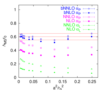
Figure 25: Comparison of $\Lambda_{\overline{MS}}$-parameters for $SU(3)$ gauge theory. The error band denotes the continuum limit result obtained by the ALPHA Collaboration Garden:2000fg . NNLO corresponds to $\mathcal{O}(\alpha^{3})$, NLO to ${\mathcal{O}}(\alpha^{2})$, bNLO and bNNLO to “boosted” NLO and NNLO, $\alpha_{L}$ to a conversion from the bare lattice coupling and $\alpha_{P}$ to the $\alpha$-values, “measured” from the logarithm of the average plaquette.

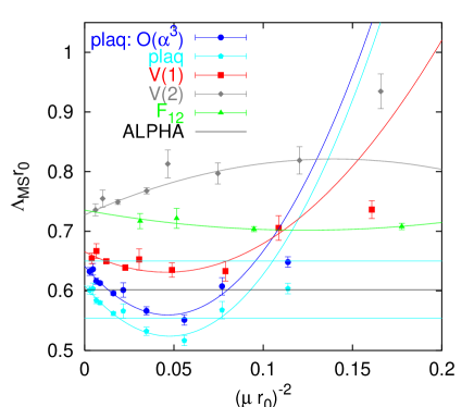
Figure 26: Comparison of $\Lambda_{\overline{MS}}$-parameters for $SU(3)$ gauge theory from different non-perturbative input quantities as a function of the scale $\mu=e^{-5/6}q^{*}$. The curves correspond to quadratic plus quartic fits in $1/\mu$ and the error band is the continuum limit ALPHA Collaboration result Garden:2000fg .

We find that the ratios between NLO and NNLO results can be brought closer to unity, both by “measuring” the coupling and by “boosting” the perturbation theory. The combination of both methods indeed brings the result in agreement with the known number (error band). Interestingly, almost all bNLO and bNNLO results are within the expected range, even at rather coarse lattice spacings.

In Tab. 23 we display values $\alpha_{\overline{MS}}(\mu)$ obtained from the short distance lattice potential and force. These are then converted into estimates of $\Lambda$-parameters and compared to the corresponding bNLO estimates from the average plaquette in Tab. 23. We also display these numbers versus the inverse momentum scale $1/\mu^{2}$ in Fig. 26. The curves represent results from phenomenological quadratic plus quartic fits in $1/(\mu r_{0})$. The $\Lambda_{\overline{MS}}r_{0}$ values resulting from these continuum limit extrapolations are displayed in the last row of the table. The results from the high $q^{*}$ quantities $V(1)$ and $\Box$ turn out to be in reasonable agreement with that from the ALPHA Collaboration, $\Lambda_{\overline{MS}}r_{0}=0.602(48)$, however, this is not the case for $F_{12}$ or $V(2)$.

Unfortunately, there exists no first principles way to estimate systematic uncertainties in any determination of $\Lambda_{\overline{MS}}$ that is partially based on perturbation theory at momenta as low as a few GeV. For instance the $F_{12}$ data exhibit a plateau for $\beta\geq 5.9$ that is in no way inferior to that obtained from the average plaquette. However, the two extrapolated values differ by almost three standard deviations of the ALPHA Collaboration result. This suggests that the good agreement obtained for the plaquette might be partly accidental. We are unaware of any convincing argument why an estimate of $\alpha_{\overline{MS}}(\mu)$ extracted from $F_{12}$ at $\beta=6.6$, i.e. $\mu r_{0}\approx 5.65$ should be less reliable than the value obtained from the plaquette at say $\beta=5.8$ ($\mu r_{0}\approx 5.4$). The same can be said about the combination $aV(2)$ at $\beta=6.6$, $\mu r_{0}\approx 12.8$ and the plaquette at $\beta=6.3$, $\mu r_{0}\approx 12.4$ and yet the former two $\beta=6.6$ estimates $\Lambda_{\overline{MS}}^{F_{12}}r_{0}=0.717(13)$ and $\Lambda_{\overline{MS}}^{V_{2}}r_{0}=0.764(24)$ happen to lie significantly higher than the known continuum limit result.

We conclude that without the comparison between predictions from different non-perturbatively obtained observables we might easily have underestimated the systematic uncertainties of the approach. Having different observables as well as the ALPHA result at hand it becomes obvious that the 4 % difference between bNLO and bNNLO estimates from the plaquette do not necessarily reflect the whole truth, but that a conservative approach would instead argue in favour of a 15 % error on the $\Lambda$-parameter in an ${\mathcal{O}}(\alpha^{2})$ determination like the above. Quantities with higher $q^{\ast}$ values are certainly likely to behave better, but incorporating a number of measurements to estimate systematic errors is prudent when such a scale setting prescription has been used.

The present article contains the NLO perturbation theory that is necessary for the use of additional short distance quantities such as $V(1)$ and the chair and parallelogram Wilson loops. The observed scattering between extrapolations from different input quantities will hopefully shrink both as finer lattices are simulated, and once higher order corrections are known for potential and force. In the meantime we quote the value,

$$\Lambda_{\overline{MS}}^{(0)}r_{0}=0.609(4)(90),$$ (110)

where the second error is systematic.

IV.2.3 Results with sea quarks

We shall limit our discussion of the fermionic case to ${\mathcal{O}}(\alpha^{2})$ since only the plaquette is known to NNLO and only for Wilson quarks at some negative mass values Alles:1998is . The fermionic correction to $c_{2}$ within Eqs. (89) – (92) can be calculated from Tab. 5 with the help of Eqs. (19) and the definitions Eqs. (14) – (16). The corrections to the potential are available in Tabs. 8 – 9, with the conventions of Eqs. (III.1) and (36) and $v_{i}=(4\pi)^{i}V_{i}$. We also include data that has been obtained by the CP-PACS Collaboration Yoshie:2000wd by combining SW fermions with the Iwasaki gluon action into the analysis. The corresponding perturbative expansion of the plaquette can be read off from Tabs. 3 and 4, with the definitions Eqs. (19) – (21). In this case $b_{1}\approx-1.2466+n_{f}K^{SW}_{1}(ma)$ Aoki:1998ar and $K_{1}$ is independent of the gauge action. We find $q^{*}a\approx 3.213$ for the plaquette. We display CP-PACS simulation parameters and results on $r_{0}/a$ and the plaquette in Tab. 25. The quark masses are obtained via Eq. (82). We set $c_{SW}=1$ in the analysis of SW-Wilson and SW-Iwasaki (SW-I) results which is consistent at NLO.

Table 25: $r_{0}/a$ and $\Box$ obtained on the CP-PACS ensemble Yoshie:2000wd .

$\beta$	$\kappa$	$ma$	$r_{0}/a$	$\Box$
1.80	0.1409	0.162	1.716(35)	0.49053(3)
1.80	0.1430	0.110	1.799(13)	0.49505(4)
1.80	0.1445	0.074	1.897(30)	0.49936(4)
1.80	0.1464	0.029	2.064(38)	0.50720(6)
1.95	0.1375	0.117	2.497(54)	0.55336(2)
1.95	0.1390	0.078	2.651(42)	0.55667(2)
1.95	0.1400	0.052	2.821(29)	0.55914(2)
1.95	0.1410	0.027	3.014(33)	0.56188(3)
2.10	0.1357	0.087	3.843(16)	0.59803(1)
2.10	0.1367	0.060	4.072(15)	0.59920(1)
2.10	0.1374	0.042	4.236(14)	0.60006(1)
2.10	0.1382	0.020	4.485(12)	0.60108(1)
2.20	0.1351	0.069	4.913(21)	0.62003(1)
2.20	0.1358	0.050	5.073(19)	0.62062(1)
2.20	0.1363	0.037	5.237(22)	0.62104(1)
2.20	0.1368	0.023	5.410(21)	0.62149(1)

Table 26: Boosted NLO estimates of $\alpha_{\overline{MS}}(\mu)$ and $\Lambda_{\overline{MS}}r_{0}$ from the average plaquette, with two flavours of Wilson quarks. $\delta\Lambda_{m}^{\Box}$ and $\delta\Lambda_{\Delta\!K_{1}}^{\Box}$ refer to the corrections, included in $\Lambda_{\overline{MS}}$, that are due to the finite quark masses and from the $ma$ dependent term $\Delta K_{1}$ alone, respectively.

$\beta$	$ma$	$\mu r_{0}$	$\alpha_{\overline{MS}}^{\Box}(\mu)$	$\Lambda_{\overline{MS}}^{\Box}r_{0}$	$\delta\Lambda_{m}^{\Box}r_{0}$	$\delta\Lambda_{\Delta\!K_{1}}^{\Box}r_{0}$
5.5	0.060	5.95 (4)	0.20925(1)	0.549(3)	+0.049	+0.056
5.5	0.040	6.48 (4)	0.20475(2)	0.564(4)	+0.038	+0.043
5.5	0.028	6.91 (5)	0.20103(3)	0.578(4)	+0.030	+0.034
5.5	0.020	7.23 (4)	0.19988(5)	0.588(4)	+0.023	+0.026
5.6	0.050	7.54 (4)	0.19405(1)	0.564(3)	+0.045	+0.051
5.6	0.040	7.81 (8)	0.19247(1)	0.570(6)	+0.038	+0.043
5.6	0.030	8.09(11)	0.19076(1)	0.575(8)	+0.031	+0.035
5.6	0.020	8.71 (4)	0.18885(1)	0.601(3)	+0.023	+0.026
5.6	0.010	9.21 (9)	0.18702(1)	0.617(6)	+0.012	+0.013

Table 27: Estimates of $\alpha_{\overline{MS}}(\mu)$ and $\Lambda_{\overline{MS}}r_{0}$ from the average plaquette, with two flavours of SW quarks. $\delta\Lambda_{m}^{\Box}$ refers to the finite quark mass correction, included in $\Lambda_{\overline{MS}}$.

$\beta$	$ma$	$\mu r_{0}$	$\alpha_{\overline{MS}}^{\Box}(\mu)$	$\Lambda_{\overline{MS}}^{\Box}r_{0}$	$\delta\Lambda_{m}^{\Box}r_{0}$
5.2	0.046	7.03 (6)	0.19109(1)	0.502(4)	+0.001
5.2	0.024	7.45 (6)	0.18903(1)	0.515(4)	+0.004
5.25	0.043	7.59 (7)	0.18568(1)	0.497(5)	+0.005
5.26	0.072	6.96 (8)	0.18647(3)	0.462(5)	+0.003
5.29	0.093	7.11 (7)	0.18407(5)	0.454(5)	+0.000
5.29	0.053	7.78(10)	0.18255(1)	0.483(7)	+0.005
5.29	0.035	8.31(13)	0.18143(1)	0.507(8)	+0.005

Table 28: Estimates of $\alpha_{\overline{MS}}(\mu)$ and $\Lambda_{\overline{MS}}r_{0}$ from the average plaquette, with “two” flavours of KS quarks.

$\beta$	$ma$	$\mu r_{0}$	$\alpha_{\overline{MS}}^{\Box}(\mu)$	$\Lambda_{\overline{MS}}^{\Box}r_{0}$	$\delta\Lambda_{m}^{\Box}r_{0}$
5.3	0.30	2.44(4)	0.3362 (15)	0.587(15)	-0.052
5.35	0.30	2.65(2)	0.3069 (14)	0.552 (7)	-0.041
5.415	0.30	2.91(8)	0.2739 (11)	0.496(16)	-0.032
5.3	0.20	2.59(8)	0.32891(55)	0.603(19)	-0.029
5.35	0.20	2.76(2)	0.29874(54)	0.551 (5)	-0.022
5.415	0.20	3.18(2)	0.26530(39)	0.508 (4)	-0.018
5.3	0.15	2.63(2)	0.32810(55)	0.595 (5)	-0.019
5.35	0.15	2.87(2)	0.29190(26)	0.549 (4)	-0.015
5.415	0.15	3.36(2)	0.25878(20)	0.510 (3)	-0.012
5.3	0.10	2.75(3)	0.31293 (1)	0.592 (6)	-0.010
5.35	0.10	3.02(2)	0.28296 (8)	0.546 (3)	-0.009
5.415	0.10	3.62(2)	0.25067 (4)	0.515 (2)	-0.007
5.5	0.10	4.58(6)	0.22136 (7)	0.488 (7)	-0.006
5.3	0.075	2.82(3)	0.30792 (8)	0.592 (7)	-0.007
5.35	0.075	3.18(2)	0.27783 (4)	0.556 (3)	-0.006
5.3	0.05	2.90(3)	0.30438(15)	0.596 (7)	-0.005
5.35	0.05	3.47(4)	0.27364 (6)	0.590 (8)	-0.003
5.415	0.05	4.02(2)	0.24217 (4)	0.530 (2)	-0.003
5.5	0.05	5.06(5)	0.21748 (1)	0.515 (5)	-0.002
5.3	0.025	3.00(2)	0.29847(15)	0.597 (4)	-0.002
5.35	0.025	3.49(3)	0.26552 (9)	0.559 (5)	-0.001
5.415	0.025	4.36(2)	0.23761 (5)	0.551 (2)	-0.001
5.5	0.025	5.62(3)	0.21541 (2)	0.559 (3)	-0.002
5.6	0.025	7.10(2)	0.19960 (3)	0.575(12)	-0.001
5.415	0.0125	4.54(3)	0.23492(13)	0.558 (4)	-0.000
5.5	0.0125	5.88(2)	0.21447 (2)	0.579 (2)	-0.000
5.6	0.08	6.03(2)	0.20033 (3)	0.494 (2)	-0.004
5.6	0.04	6.71(3)	0.19975 (1)	0.545 (3)	-0.002
5.6	0.02	7.15(2)	0.19929 (1)	0.577 (2)	-0.001
5.6	0.01	7.38(2)	0.19916 (1)	0.594 (2)	-0.000

Table 29: Estimates of $\alpha_{\overline{MS}}(\mu)$ and $\Lambda_{\overline{MS}}r_{0}$ from the average plaquette, with two flavours of SW quarks and Iwasaki glue.

$\beta$	$ma$	$\mu r_{0}$	$\alpha_{\overline{MS}}^{\Box}(\mu)$	$\Lambda_{\overline{MS}}^{\Box}r_{0}$
1.80	0.162	2.396(49)	0.28681(2)	0.445 (9)
1.80	0.110	2.512(18)	0.28378(3)	0.457 (4)
1.80	0.073	2.649(42)	0.28091(3)	0.473 (8)
1.80	0.029	2.882(53)	0.27573(4)	0.497 (9)
1.95	0.117	3.487(75)	0.24623(1)	0.477(10)
1.95	0.078	3.702(59)	0.24418(1)	0.497 (8)
1.95	0.052	3.939(40)	0.24265(1)	0.522 (6)
1.95	0.027	4.209(46)	0.24096(2)	0.549 (6)
2.10	0.087	5.366(22)	0.21910(1)	0.558 (3)
2.10	0.060	5.686(21)	0.21841(1)	0.586 (2)
2.10	0.042	5.915(20)	0.21790(1)	0.606 (2)
2.10	0.020	6.263(17)	0.21729(1)	0.637 (2)
2.20	0.069	6.860(29)	0.20616(1)	0.608 (3)
2.20	0.050	7.084(27)	0.20582(1)	0.625 (3)
2.20	0.037	7.313(31)	0.20558(1)	0.643 (3)
2.20	0.023	7.554(29)	0.20531(1)	0.662 (3)

Table 30: Boosted NLO estimates of $\Lambda_{\overline{MS}}^{(2)}r_{0}$ for Wilson quarks from the average plaquette, $aV(1)$, $aV(2)$ and $F_{12}$, respectively. The errors are purely statistical.

$\beta$	$ma$	$\Lambda_{\overline{MS}}^{\Box}r_{0}$	$\Lambda_{\overline{MS}}^{V_{1}}r_{0}$	$\Lambda_{\overline{MS}}^{V_{2}}r_{0}$	$\Lambda_{\overline{MS}}^{F_{12}}r_{0}$
5.5	0.060	0.549(3)	0.616 (5)	0.786 (8)	0.687 (8)
5.5	0.040	0.564(4)	0.628 (5)	0.784 (8)	0.690 (8)
5.5	0.028	0.578(4)	0.641 (6)	0.790 (8)	0.697 (8)
5.5	0.020	0.588(4)	0.650 (6)	0.788 (8)	0.693 (8)
5.6	0.050	0.564(3)	0.621 (5)	0.759 (7)	0.691 (7)
5.6	0.040	0.570(6)	0.627 (8)	0.758(11)	0.686(11)
5.6	0.030	0.575(8)	0.634(10)	0.755(14)	0.678(15)
5.6	0.020	0.601(3)	0.659 (4)	0.784 (6)	0.709 (7)
5.6	0.010	0.617(6)	0.675 (8)	0.805(13)	0.734(15)

Table 31: Estimates of $\Lambda_{\overline{MS}}^{(2)}r_{0}$ for SW quarks.

$\beta$	$ma$	$\Lambda_{\overline{MS}}^{\Box}r_{0}$	$\Lambda_{\overline{MS}}^{V_{1}}r_{0}$	$\Lambda_{\overline{MS}}^{V_{2}}r_{0}$	$\Lambda_{\overline{MS}}^{F_{12}}r_{0}$
5.2	0.046	0.502(4)	0.537(5)	0.653 (8)	0.672 (9)
5.2	0.024	0.515(4)	0.546(5)	0.655 (7)	0.670(10)
5.2	0.018	—	0.559(6)	0.666 (8)	0.678(10)
5.26	0.072	0.462(5)	0.500(7)	0.611(10)	0.645(12)
5.29	0.093	0.454(5)	0.496(6)	0.605 (8)	0.648(11)

Table 32: Estimates of $\Lambda_{\overline{MS}}^{(2)}r_{0}$ for KS quarks.

$\beta$	$ma$	$\Lambda_{\overline{MS}}^{\Box}r_{0}$	$\Lambda_{\overline{MS}}^{V_{1}}r_{0}$	$\Lambda_{\overline{MS}}^{V_{2}}r_{0}$	$\Lambda_{\overline{MS}}^{F_{12}}r_{0}$
5.3	0.300	0.587(15)	0.684(19)	—	—
5.3	0.200	0.603(19)	0.699(27)	—	—
5.3	0.150	0.595 (5)	0.694 (8)	—	—
5.3	0.100	0.592 (6)	0.683(13)	—	—
5.3	0.075	0.592 (7)	0.699 (8)	—	—
5.3	0.050	0.596 (7)	0.696(11)	—	—
5.3	0.025	0.697 (4)	0.692 (6)	—	—
5.35	0.300	0.552 (7)	0.670 (7)	—	—
5.35	0.200	0.551 (5)	0.661 (7)	—	—
5.35	0.100	0.546 (3)	0.650 (6)	0.840(31)	—
5.35	0.075	0.556 (3)	0.664 (6)	0.900(33)	—
5.35	0.050	0.590 (8)	0.702(12)	0.959(34)	0.434(71)
5.35	0.025	0.559 (5)	0.660 (8)	0.904(25)	0.526 (9)
5.415	0.300	0.496(16)	0.618(19)	0.879(76)	—
5.415	0.200	0.508 (4)	0.626 (7)	0.846(26)	0.477(13)
5.415	0.150	0.510 (3)	0.627 (5)	0.854(25)	0.517(12)
5.415	0.100	0.515 (2)	0.620 (5)	0.881(18)	0.561 (7)
5.415	0.050	0.530 (2)	0.625 (4)	0.836(11)	0.596 (7)
5.415	0.025	0.551 (2)	0.634 (4)	0.853(11)	0.630 (7)
5.415	0.0125	0.558 (4)	0.634 (6)	0.840(13)	0.635(10)
5.5	0.100	0.488 (7)	0.580 (9)	0.787(14)	0.623(11)
5.5	0.050	0.515 (5)	0.592 (6)	0.772 (8)	0.631 (7)
5.5	0.025	0.559 (3)	0.629 (4)	0.800 (7)	0.661 (7)
5.5	0.0125	0.579 (2)	0.645 (3)	0.814 (5)	0.676 (5)
5.6	0.080	0.494 (2)	0.564 (2)	0.717 (4)	0.627 (4)
5.6	0.040	0.545 (3)	0.607 (3)	0.756 (5)	0.662 (5)
5.6	0.020	0.577 (2)	0.634 (2)	0.776 (4)	0.676 (4)
5.6	0.010	0.594 (2)	0.650 (2)	0.783 (4)	0.676 (4)

Table 33: Chirally extrapolated $a/r_{0}$ values and extrapolations of $\Lambda_{\overline{MS}}^{(2)}r_{0}$, according to Eq. (111).

Action	$\beta$	$a/r_{0}$	$c$	$[\Lambda_{\overline{MS}}^{(2)}r_{0}](0)$	$\chi/{N_{DF}}$
Wilson	5.5	0.178(4)	-0.271(17)	0.613(3)	0.51/2
Wilson	5.6	0.148(3)	-0.335(47)	0.639(7)	1.67/2
SW	5.2	0.185	-0.136	0.532	$N_{DF}=0$
SW	5.29	0.162(4)	-0.198(23)	0.542(9)	0.48/1
KS	5.415	0.312(2)	-0.311(30)	0.573(3)	0.56/1
KS	5.5	0.236(6)	-0.508(38)	0.605(3)	1.06/1
KS	5.6	0.194(1)	-0.371 (8)	0.613(1)	0.16/1
SW-I	1.8	0.460(11)	-0.251(34)	0.508(7)	0.78/2
SW-I	1.95	0.312 (5)	-0.358(34)	0.575(6)	0.83/2
SW-I	2.1	0.213 (1)	-0.327(12)	0.666(3)	2.08/2
SW-I	2.2	0.177 (1)	-0.254(18)	0.692(4)	2.32/2

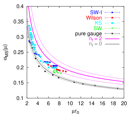
Figure 27: Comparison between bNLO $\alpha_{\overline{MS}}$ estimates from pure gauge theory simulations and simulations with $n_{f}=2$ Wilson, KS and SW quarks, the latter with Wilson and Iwasaki (SW-I) gluon actions. The $n_{f}=0$ error band corresponds to the ALPHA result $\Lambda_{\overline{MS}}=0.602(48)r_{0}^{-1}$ while the $n_{f}=2$ band corresponds to the four-loop running with $\Lambda_{\overline{MS}}^{(2)}=0.69(15)$.

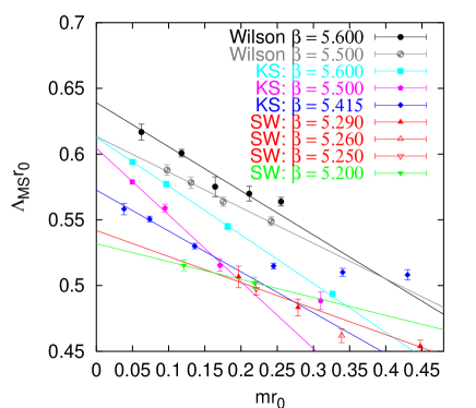
Figure 28: Chiral extrapolations of $\Lambda_{\overline{MS}}^{(2)}r_{0}$ at finite lattice spacings for the Wilson gluonic action combined with the three different fermionic actions.

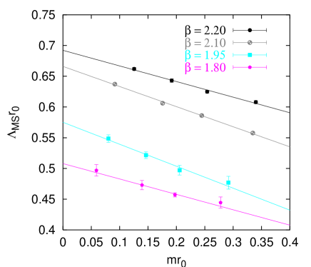
Figure 29: Chiral extrapolations of $\Lambda_{\overline{MS}}^{(2)}r_{0}$ at finite lattice spacings for the SW-I action.

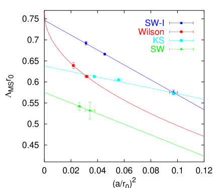
Figure 30: Attempts of a continuum limit extrapolation (linear in $a/r_{0}$ for Wilson and quadratic for KS and SW quarks) of $\Lambda_{\overline{MS}}^{(2)}r_{0}$ from the available “world lattice data”.

We display our results on $\alpha_{\overline{MS}}(\mu)$ as well as on $\Lambda_{\overline{MS}}r_{0}$ in Tabs. 26 – 29. $\delta\Lambda_{m}^{\Box}$ refers to the contribution to the $\Lambda_{\overline{MS}}$-parameters due to the mass dependence of the coefficients $c_{2}$, $b_{1}$ (through $\Delta K_{1}$) and is included into the $\Lambda_{\overline{MS}}$ estimates. This mass dependence has not been considered prior to the present study. For SW and KS fermions the effect turns out to be of the order of the statistical uncertainty as long as $ma<0.1$. However, for Wilson fermions this is a substantial effect, ranging from 10 % at $ma\approx 0.06$ to 2 % at $ma\approx 0.01$. In this case the main effect is due to the term $\Delta K_{1}(ma)$ in the matching between lattice and $\overline{MS}$ scheme and we hence conclude that un-improved Wilson fermions are not particularly well suited for unambiguous determinations of the running coupling, unless data at rather small quark masses are available. We have neglected the mass dependence in our analysis of the SW-I data (Tab. 29), which is equally small as in the SW-Wilson case.

We use our perturbative result on the potential to estimate the ratio $\Lambda_{\overline{MS}}r_{0}$ from the potential $aV(1)$, $aV(2)$ and force $F_{12}$ for the three $n_{f}=2$ data sets with Wilson glue. The resulting numbers are compared to the results from the plaquette in Tabs. 30 – 32. Like in the quenched case the estimates from $V(2)$ consistently turn out to be bigger by about 15 %, in comparison to those obtained from $V(1)$ or the plaquette, however, in the case of KS quarks the estimates from $F_{12}$ are somewhat more in line with those from the plaquette. At present we do not have data at sufficiently many different lattice spacings for a detailed comparison like the one presented in Fig. 26 for the $n_{f}=0$ case. Hence, we will only use the most ultra violet quantity, the average plaquette, to extract the $n_{f}=2$ $\Lambda$-parameter and assume a systematic uncertainty of 15 % due to higher order perturbative corrections, based on our study of the pure gauge case as well as on the numbers in Tabs. 30 – 32.

In Fig. 27 we compare our $n_{f}=2$ estimates on $\alpha_{\overline{MS}}(\mu)$ from the plaquette to the $n_{f}=0$ results. Due to the variation in the sea quark masses, action and lattice spacings used, the $n_{f}=2$ points scatter around quite a bit but yield consistently larger values of $\alpha$, compared to the quenched case as already observed in lattice simulations of the static potential, for instance in Ref. Bali:2000vr as well as in Sec. IV.3 below. It is also clear from the figure that at present the $\mu$-window covered by $n_{f}=2$ results is much smaller than the one available in pure gauge studies.

Since chiral symmetry is explicitly broken for the fermionic actions used we should first extrapolate our $\Lambda_{\overline{MS}}^{(2)}$ estimates obtained at similar quark masses in physical units $mr_{0}$ to the continuum limit, before attempting a chiral extrapolation: $m\rightarrow m_{u},m_{d}\approx 0$. Due to the small range of lattice spacings covered by the presently available data, however, we are forced to interchange the ordering of these two limits: after discarding lattices with $2.5\,a>r_{0}$, i.e. the KS data with $\beta<5.415$ or $ma>0.05$, we extrapolate in $\Lambda_{\overline{MS}}^{(2)}r_{0}$ at fixed $\beta$-values to small quark masses and subsequently send the lattice spacing to zero.

The chiral extrapolations are illustrated in Fig. 28 for Wilson glue and in Fig. 29 for the SW-I action. We include the $\beta=1.8$ data points into the latter figure but we will discard these coarse lattice results from our continuum limit extrapolation. The last column of Tab. 30 reveals that the slopes of $\Lambda_{\overline{MS}}^{(2)}r_{0}$ as a function of $mr_{0}$ would have been much steeper for Wilson fermions had we neglected the $ma$ dependence of the matching between lattice and $\overline{MS}$ schemes. In the course of each extrapolation the lattice spacing in physical units $a/r_{0}$ changes. However, $\Lambda$ is no spectral quantity and there is no theoretical handle on the functional form of such an extrapolation anyway. We find linear fits,

$$\left[\Lambda_{\overline{MS}}^{(2)}r_{0}\right](mr_{0})=\left[\Lambda_{\overline{MS}}^{(2)}r_{0}\right](0)+c\,mr_{0},$$ (111)

with parameters $[\Lambda_{\overline{MS}}^{(2)}r_{0}](0)$ and $c$, to be consistent with the $mr_{0}<0.25$ ($mr_{0}<0.35$ for the SW-I action) data. The resulting parameter values as well as $a/r_{0}(m=0)$ can be found in Tab. 33. For the SW data at $\beta=5.20$ no fit is possible since $N_{DF}=0$ and at $\beta=5.29$ we included a rather heavy mass, $mr_{0}\approx 0.45$.

Finally we attempt a continuum limit extrapolation in Fig. 30, where we have generously estimated error bars for the SW quarks at $\beta=5.20$. The lines represent extrapolations, linear in $a/r_{0}$ for Wilson fermions and quadratic in $a/r_{0}$ for KS and SW quarks. The extrapolated values are $\Lambda_{\overline{MS}}^{(2)}r_{0}=0.638(3)$ with $\chi^{2}/N_{DF}=0.75/1$ for KS quarks, $\Lambda_{\overline{MS}}^{(2)}r_{0}\approx 0.764$ and $\Lambda_{\overline{MS}}^{(2)}r_{0}\approx 0.575$ for Wilson and SW fermions, respectively, in which cases $N_{DF}=0$. For the SW-I action we obtain $\Lambda_{\overline{MS}}^{(2)}r_{0}=0.747(2)$ with $\chi^{2}/N_{DF}=0.05/1$. As a final result we quote the (unweighted) average of the KS and SW-I data sets,

$$\Lambda_{\overline{MS}}^{(2)}r_{0}=0.69\pm 0.15,$$ (112)

where the error estimate reflects the uncertainties due to higher order perturbative corrections as well as in the extrapolations, both chiral and to the continuum limit.

The above number should be related to the recent more optimistic estimate $\Lambda_{\overline{MS}}^{(2)}r_{0}=0.553(34)$ by the QCDSF and UKQCD collaborations Booth:2001qp which is based on the UKQCD SW data alone. Note that their result agrees with our above value, $\Lambda_{\overline{MS}}^{(2)}r_{0}\approx 0.575$, obtained from the same SW data set by use of somewhat different methods in the conversion between schemes and extrapolations. For instance in Ref. Booth:2001qp $\alpha_{\overline{MS}}(\mu)$ was extracted at NNLO, estimating the as yet unknown NNLO fermionic contribution to the plaquette, while we consistently worked at NLO.

Fig. 30 paints a superficially disappointing picture for universality of the continuum limit. Universality absolutely must hold for lattice field theory to be a worthwhile exercise, so one might be concerned about the large difference in particular between the two different results obtained with SW fermions. While we try to estimate systematics by incorporating this difference into our error, it is interesting to consider how one could expect the figure to mature as improved data from future simulations become available.

Firstly, we note that the KS and SW-I continuum limit extrapolations are much better controlled than those for Wilson or SW quarks with Wilson glue, due to the availability of an additional data point. There are sizable ${\mathcal{O}}(a^{2})$ corrections to the current KS and SW data. The Wilson continuum limit result has been obtained by drawing a straight line through two data points but there is no reason to believe ${\mathcal{O}}(a^{2})$ corrections to be any smaller (nor indeed any larger) in this case than in the SW and KS cases. Likewise, it is not clear whether part of the large slope of the SW-I data set (which is only perturbatively improved such that ${\mathcal{O}}(\alpha_{L}a)$ corrections are still present) might be due to a residual linear contribution. One might hope that the scatter of the results will be reduced by future data at different lattice spacings that would allow us to discriminate between linear and quadratic terms.

Secondly, we note that perturbative coefficients for the effects of the clover term in the SW action are particularly large throughout the literature, and refer the reader to Eq. (A.2) for an example of an ${\mathcal{O}}(\alpha^{2})$ coefficient and Eqs. (A.2) and (A.2) for ${\mathcal{O}}(\alpha^{3})$. There is no automatism that guarantees ${\mathcal{O}}(\alpha^{3})$ corrections to the plaquette in determinations of $\alpha_{\overline{MS}}$ to be small, just because this happened to be the case in the quenched theory with Wilson glue. Given the experience of the large $c_{SW}^{\nu}$ corrections we find it at least plausible that perturbative corrections to the SW determinations are larger than for the two other formulations. A calculation of these might result in a better agreement between the different continuum extrapolations too.

We remain confident that a combination of more lattice data and higher order perturbative calculations will greatly reduce the systematic spread shown in Fig. 30. Of course eventually the ordering of chiral and continuum limit extrapolations should be interchanged, unless data with chirally symmetric lattice fermions become available.

We finally note that efforts are on the way of calculating the $n_{f}=2$ $\Lambda$-parameter with the help of finite size scaling techniques in the Schrödinger functional scheme. At present the error from this approach DellaMorte:2002vm is of ${\mathcal{O}}(50\mbox{\%})$ and the scale has still to be related to a physical quantity like $r_{0}$ or $f_{\pi}$, however, some improvement can be expected in the near future.

IV.2.4 Implications for the “real” world

Running the estimate $\Lambda_{\overline{MS}}^{(2)}r_{0}=0.69(15)$ to the mass of the $Z$ vector boson $m_{Z}\approx 91.2$ GeV results in the value,

$$\alpha_{\overline{MS}}^{(2)}(m_{Z})=0.0945(30)(7),$$ (113)

where the second error that is smaller than 1 % is due to the 5 % scale ambiguity Bali:1997am in the phenomenological value $r_{0}\approx 0.5$ fm. This subdominant uncertainty can be reduced by using a quantity directly accessible in experiment like $f_{\pi}$ or $m_{N}$ to set the scale. Nature of course does not contain two but five quark flavours lighter than the $Z$ boson and we have to address this problem if we intend to produce numbers that have phenomenological relevance.

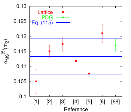
Figure 31: Our estimate of $\alpha_{\overline{MS}}^{(5)}$ (error band), in comparison with numbers quoted in previous lattice studies as well as with the average from the “Review of Particle Physics” (PDG).

The main difficulty of a QCD prediction is the effect of the strange quark. Given that we cannot resolve the shift between $\Lambda^{(0)}_{\overline{MS}}r_{0}=0.60(5)$ and $\Lambda^{(2)}_{\overline{MS}}r_{0}=0.69(15)$ within the errors, for the moment being we assume that the strange quark which is heavier than the up and the down quarks anyway will not have a large impact on this ratio either and guess $\Lambda^{(3)}_{\overline{MS}}r_{0}\approx\Lambda^{(2)}_{\overline{MS}}r_{0}$. However, we try to incorporate the uncertainty of this assumption (as well as the scale error of $r_{0}$) by somewhat inflating the systematic error:

$$\Lambda^{(3)}_{\overline{MS}}=270(70)\,\,\mbox{MeV}.$$ (114)

Our result of Sec. III.5 indicates that a perturbative matching of the $n_{f}=3$ and $n_{f}=4$ couplings around the charm threshold should be reliable. Further, the difference between a three and a four-loop $\overline{MS}$ running from a scale of 1.1 GeV upwards corresponds to a relative shift in $\alpha_{\overline{MS}}$ at the $Z$ resonance of only 0.26 %. Hence, we perturbatively match the coupling at the charm and bottom thresholds. We allow pole masses $1.1$ GeV$<m_{c}<1.5$ GeV and 4.4 GeV $<m_{b}<5.0$ GeV and arrive at the estimate,

$$\alpha_{\overline{MS}}^{(5)}(m_{Z})=0.1133(59),$$ (115)

using the four-loop $\beta$-function. The effect of varying the respective quark masses $m_{c}$ and $m_{b}$ as well as differences between a three and four-loop running of the coupling have been added linearly in the above error.

The result is compatible with the average quoted in the “Review of Particle Physics” Hagiwara:pw : $\alpha_{\overline{MS}}^{(5)}(m_{Z})=0.1172(20)$ but lower than results from D0/CDF or LEP experiments, a tendency that is consistent with previous lattice estimates El-Khadra:1992vn ; davi1 ; davi2 ; Spitz:1999tu ; Booth:2001qp . In Fig. 31 we relate various lattice studies in chronological order to ours. We find that, although all lattice results on this quantity El-Khadra:1992vn ; davi1 ; davi2 ; Spitz:1999tu ; Booth:2001qp ; davi3 (as well as the PDG world average Hagiwara:pw ) lie within the error bars that we obtain, many of the previous numbers turn out to be incompatible with each other, within their quoted uncertainties. For instance we obtain a $\chi^{2}/N_{DF}=17.2/5$ when averaging the six lattice results, and this assuming that the quoted errors, that are dominated by systematics, only represent one standard deviation!

The least well controlled step in our prediction Eq. (115) is certainly the extrapolation $n_{f}=0,2\longrightarrow n_{f}=3$. A first lattice study with “$n_{f}=3$” exists davi3 , however, it is too early to investigate quark mass effects and to attempt a continuum limit extrapolation in this case. Once lattice results with 2+1 quark flavours of a similar quality as those analysed here become available a determination of $\alpha_{\overline{MS}}(m_{Z})$ with about 4 % accuracy using the methods explored above should become realistic, and by both, a full fledged ${\mathcal{O}}(\alpha^{3})$ calculation in lattice perturbation theory and more simulation points that would allow for a better controlled continuum limit extrapolation this error should be reducible to 1 – 2 % within the next few years.

We experienced that systematic errors are easily underestimated in this kind of study, in particular since neither the size of higher order perturbative corrections nor the functional form of the chiral and continuum limit extrapolations are fully controlled. However, using a set of different lattice observables and actions certainly helps in arriving at realistic error estimates. Perturbation theory is naturally most reliable when the scales involved are high and it is very expensive to increase the energy $a^{-1}$ in lattice simulations, at least if one keeps the simulation volume fixed in physical units. This makes the average plaquette a particularly valuable quantity in studies like the present one. Future predictions might benefit if lattice data on the plaquette, not only in the fundamental but also in the adjoint and higher representations, were available as well as data on other short distance quantities like the “chair”, the “parallelogram” and the “rectangle”.

IV.3 Comparison to the non-perturbative static potential

We shall compare our perturbation theory results with data from simulations of QCD without and with sea quarks. First we explain what we mean by boosted and tadpole improved boosted perturbation theory in the present context. Next we investigate different possibilities to parametrize the pure gauge static potential at short distances, based on our results of Sec. III. We conclude with an attempt to resolve the different running of the coupling when including sea quarks from non-perturbative data.

IV.3.1 Parametrizations of the potential

In what follows we will refer to the parametrization

$$aV({\mathbf{R}}a)=g^{2}V_{1}({\mathbf{R}})$$ (116)

with $V_{1}$ defined in Eq. (30) [and Eq. (34)] as leading order (LO). Apart from a different value of $g^{2}=6/\beta$ this result does not depend on $n_{f}$. The NLO result can be found in Eqs. (31) – (36). The LO result above corresponds to

$$aV(Ra)-aV_{S}(a)\longrightarrow-C_{F}\frac{g^{2}}{4\pi R}\quad(R\rightarrow\infty),$$ (117)

where $aV_{S}=C_{F}g^{2}\times 0.252731\ldots$ while the parametrizations of the NLO and NNLO curves in the $R\gg 1$ limit with and without massive sea quarks can be found in Appendix A.4. In the pure gauge case we will also compare against NNLO expectations for which the small $R$ lattice effects have not yet been calculated. When including fermions this is not possible since even in the massless case the contribution to the self energy is only known to NLO.

In addition to expansions in terms of the bare coupling we shall also compare against “boosted” perturbation theory expectations. In this case we use the $\Lambda_{\overline{MS}}$ values of Tabs. 24 and 26, calculated from the respective plaquette at NLO as input. Since we shall compute the coupling $\alpha_{V}(q)$ at NNLO this is somewhat inconsistent. However, we also aim at a comparison with the fermionic case where such a determination of the $\Lambda$-parameter is at present only possible at NLO and prefer to compare like with like. As we have seen above, the numerical difference between NLO and NNLO turns out to be small anyway for this quantity. Using $\Lambda_{\overline{MS}}r_{0}$ as input we numerically run $\alpha_{\overline{MS}}(\mu)$ to the required scales $\mu=e^{-5/6}q^{*}$, according to the four-loop $\beta$-function. Some of the respective $aq^{*}({\mathbf{R}})$ values can be read off Tab. 11 and for large $R$ we employ the parametrization Eq. (60). Slightly deviating from Sec. IV.2, the resulting $\alpha_{\overline{MS}}(\mu)$ is then always converted into $\alpha_{V}(q^{*})$ at the two loop level [${\mathcal{O}}(g^{6})$], at bLO as well as at bNLO and bNNLO, via Eqs. (153) – (A.3) and Eq. (167). This means that what we call bLO includes some NLO and NNLO contributions and bNLO includes a conversion from the $\overline{MS}$ to the $V$ scheme at NNLO. However, the conversion from the momentum space continuum to the position space lattice potential is done at the order indicated.

Finally, we introduce “tadpole improved” boosted perturbation theory. We start from the observation that each link that appears within any lattice observable contains classes of tadpole diagrams that are lattice specific. We try to cancel these ultra violet contributions in part by a non-perturbative prescription Parisi:1980pe ; lepage : the second of the two Wilson loops that appear within the difference $aV(a{\mathbf{R}})=\lim_{T\rightarrow\infty}\{\ln[W({\mathbf{R}},T)]-\ln[W({\mathbf{R}},T+1)]\}$ contains two more links than the first one. We hence prefer to perturbatively expand the combination $aV(a{\mathbf{R}})+\ln\Box/2$ instead, within which the net number of links is zero. We have already made use of this trick in Eq. (74). Finally, we reexpress the result in terms of $\alpha_{V}(q^{*}_{N})$, boosting our perturbative series, where the new $q^{*}_{N}({\mathbf{R}})$ values can easily be calculated from those of the potential $q^{*}({\mathbf{R}})$ and the plaquette $q^{*}_{\Box}$:

$$\ln(aq^{*}_{N}({\mathbf{R}}))=\frac{\ln[aq^{*}({\mathbf{R}})]V_{1}({\mathbf{R}})-\ln(aq^{*}_{\Box})c_{1}/2}{V_{1}({\mathbf{R}})-c_{1}/2}.$$ (118)

The $\alpha_{V}(q^{*}_{N})$ are then obtained as described above. We shall refer to this third method as tbLO, tbNLO and tbNNLO, depending on the order of the conversion from $\alpha_{V}[q^{*}_{N}({\mathbf{R}})]$ to $aV({\mathbf{R}})$.

IV.3.2 Pure gauge theory

In Fig. 32 we compare LO, NLO, NNLO and bLO, bNLO and bNNLO expectations against the static potential at $\beta=6.0$. At this lattice spacing we use $\Lambda_{\overline{MS}}r_{0}=0.562(3)$ and there is no free parameter. The un-boosted results come closer to the non-perturbative data as the order of the calculation increases but even at NNLO only about half of the potential can be explained, even at distances as short as $R=1$. The boosted results are more in line with the data but still only on a very qualitative level at best. It is also obvious that if one tuned the $\Lambda$-parameter such that $V(1)$ is reproduced, $V(2)$ would be undershot, in agreement with our experience from Sec. IV.2 above. We can define an effective Coulomb coupling,

$$e(R)=-R[aV(R)-aV_{S}],$$ (119)

and find $e\approx 0.106$ at LO while $e(3)\approx 0.19$ and $e(3)\approx 0.26$ at NLO and NNLO, respectively. Finally, bNLO results in $e(3)\approx 0.49$.

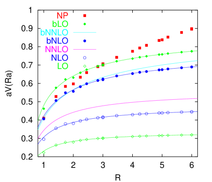
Figure 32: Comparison between quenched lattice data at $\beta=6.0$ and boosted (b) and un-boosted LO, NLO and NNLO perturbative potentials. The curves are the large $R$ expectations from continuum perturbation theory.

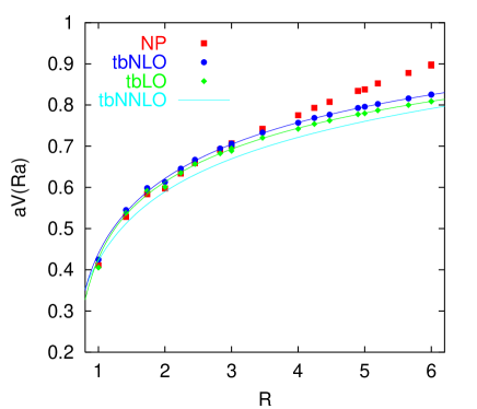
Figure 33: The non-perturbative potential at $\beta=6.0$, in comparison with boosted and tadpole improved perturbation.

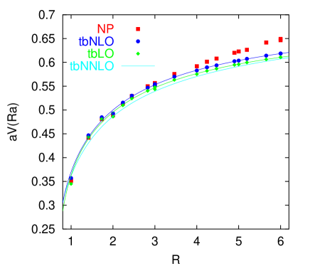
Figure 34: The same as Fig. 33 at $\beta=6.4$.

Next in Fig. 33 we try out the tbLO, tbNLO and tbNNLO parametrizations and indeed tadpole improvement vastly reduces the difference with the NP potential. To exclude that this is just accidental we also display a comparison with the potential at $\beta=6.4$ in Fig. 34 where the plaquette yields $\Lambda_{\overline{MS}}r_{0}=0.603(10)$, and with the smaller gauge coupling the situation becomes even more convincing. It turns out to be absolutely essential to compare like with like. Contrary to previous claims Bali:1999ai ; Necco:2001gh not only the force but also the short range potential can be understood in terms of perturbation theory, provided that the self energy contribution is dealt with in a consistent way: when comparing with NP lattice results the self energy should not be subtracted from the perturbative expansion while when matching with the $\overline{MS}$ scheme in which $V_{S}^{\overline{MS}}=0$ by definition it has to be subtracted at the same scales $\mu(r)$ at which the interaction energy $V_{\mbox{\scriptsize int}}(r)=V(\mu;r)-V_{S}(\mu)$ is calculated, to avoid renormalon ambiguities. A similar observation has been made in a recent comparison with continuum perturbation theory in a renormalon based approach Pineda:2002se . In Ref. Bali:1999ai a comparison was made between the NP lattice potential at short distances and the perturbative $\overline{MS}$ scheme prediction. In this study one and the same perturbative self energy had been used at all distances, which was obtained from a fit to the data, and consequently, no agreement was found.

Figure 35: Non-Perturbative minus perturbative potentials at $\beta=6.4$, together with a quadratic fit, Eq. (120). The distance $r=0.4\,r_{0}\approx 1\,\mbox{GeV}^{-1}$ corresponds to about 4 lattice spacings.

In Fig. 35 we display the difference between non-perturbative and perturbative potentials, $\Delta V(r)=V(r)-V^{\mbox{\scriptsize tbNLO}}(r)$ for the example of $\beta=6.4$ as a function of $R=r/a$ in physical units $r_{0}/a=9.89(16)$. Within the statistical errors of the non-perturbative potential all points lie on a smooth curve indicating that the lattice effects are accounted for by the perturbative result. However, there are deviations between prediction and lattice data: at short distances we overestimate the NP potential by 30 MeV and around 0.3 fm we underestimate the result by 110 MeV. We fit the difference for $r<0.61\,r_{0}\approx 0.3$ fm by the phenomenological ansatz,

$$\Delta V(r)=b+cr^{2}$$ (120)

with $b=-0.068(3)\,r_{0}^{-1}$, $c=0.99(6)\,r_{0}^{-3}$ and $\chi^{2}/N_{DF}=18.2/17$. Allowing for an additional linear term does not improve the quality of the fit and the term turns out to be in agreement with zero: unlike in Ref. Bali:1999ai no linear term is required at short distances to understand the data and this without any free parameter in the computation of $\Delta V(r)$! We notice that the coefficient $c\approx(1.6\Lambda_{\overline{MS}})^{3}$ is of order one in units of the QCD $\Lambda$-parameter.

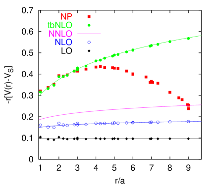
Figure 36: The running of the Coulomb coupling at $\beta=6.6$, where $5.1\,a\approx 0.4\,r_{0}\approx 0.2$ fm $\approx 1$ GeV^-1. We have subtracted the value $aV_{S}^{\mbox{\scriptsize tbNLO}}\approx 0.65$ from the non-perturbative potential.

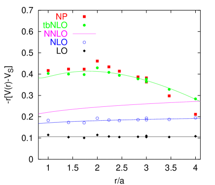
Figure 37: The same as Fig. 36 at $\beta=6.0$, where $2.1\,a\approx 0.4\,r_{0}$ and we subtract the estimate $aV_{S}^{\mbox{\scriptsize NP}}\approx 0.83$.

In view of our plan to resolve the differences in the running of the coupling between quenched and un-quenched simulations, in Fig. 36 we display the dimensionless combination $e(r/a)$ of Eq. (119) for $\beta=6.6$ where $5.1\,a\approx 0.4\,r_{0}\approx 1\,\mbox{GeV}^{-1}$. At this $\beta$ value the average plaquette yields $\Lambda_{\overline{MS}}r_{0}=0.601(7)$. We have also included bare LO, NLO and NNLO results for comparison. The self energies have been subtracted from all perturbative potentials, LO, NLO, NNLO as well as tbNLO at the respective orders in perturbation theory. As what we are doing is a linear transformation we do not wish to subtract different $V_{S}$ values from the NP and tbNLO potentials which would spoil the qualitative agreement between the results found above. Ideally one would subtract a non-perturbatively determined $V_{S}$ which then guarantees scaling between different NP data sets. The difference between NP and tbNLO however will then result in the tbNLO coupling to diverge linearly at large $R$ where perturbation theory will become unreliable anyway. In the absence of a non-perturbative determination of $V_{S}$ we will take the $\beta=6.6$ tbNLO value $aV^{\mbox{\scriptsize tbNLO}}_{S}\approx 0.650$ as an estimate which is indeed close at least to the tbNNLO result $aV^{\mbox{\scriptsize tbNNLO}}_{S}\approx 0.670$. Doing this means that the tbNLO Coulomb coupling will increase logarithmically with $R$ and no linear term is present.

In the figure we see a gap opening up between NP and tbNLO potentials for $Ra>4a\approx 0.15$ fm. The NP data starts diverging towards negative values, which is expected as $e(r)\rightarrow-\sigma r^{2}$ as $r\rightarrow\infty$ where $\sigma$ denotes the string tension. In addition, our estimate of an NP self energy might be wrong by a few per cent which will result in an unwanted linear contribution to $e$. We find relatively large values of the Coulomb coupling, $e\approx 0.4$, that naturally disagree with $e\approx 0.3$ as obtained from phenomenological fits to a Cornell type potential Bali:2000vr ; Bali:2000gf , $aV(R)=V_{0}-e/R+a^{2}\sigma\,R$, in which the linear confining term contributes at all distances: the parameter $e$ within this parametrization can only be interpreted as a Coulomb coupling at distances $r\ll\sqrt{\sigma}$. We observe that the running of the coupling is quite steep at short distances which provides us with hope that differences between the quenched and un-quenched $\beta$-functions can be resolved from simulation data.

In Fig. 37 we display the same comparison for a similar $R$ range in physical units at $\beta=6.0$ where $2.1\,a\approx 0.4\,r_{0}\approx 1\,\mbox{GeV}^{-1}$. In this case the difference between tbNLO and tbNNLO self energies is 15 % such that we cannot regard these values as reliable anymore. Instead we compute $a^{6.0}V_{S}^{6.0}=a^{6.0}V^{6.0}(r_{0})-(R_{0}^{6.6}/R_{0}^{6.0})a^{6.6}[V^{6.6}(r_{0})-V_{S}^{6.6}]$, where the superscripts refer to the respective $\beta$ values, and add this non-perturbative difference to the $\beta=6.6$ $aV_{S}$ estimate above. In doing this we arrive at $aV_{S}^{\mbox{\scriptsize NP}}\approx 0.83$ which we subtract from both NP and tbNLO data sets. Now at large $R$ the tbNLO coupling will diverge linearly towards negative values as our $V_{S}^{\mbox{\scriptsize NP}}$ estimate differs from $V_{S}^{\mbox{\scriptsize tbNLO}}$ by as much as $0.35\,a^{-1}$. It is obvious when comparing for instance the dimensionless NP couplings at $R\approx 3.5$ with $R\approx 8.5$ that both NP data sets scale nicely. We see however that at short distances the agreement with the perturbative expectation at $\beta=6.0$ is somewhat worse than that at $\beta=6.6$ above. The gap between NP and tbNLO curves opens up in the same region in lattice units, around $R\approx 4$, which corresponds to a larger distance in physical units. Since the perturbative expectation decreases at large $r$ only because of the difference between $aV_{S}^{\mbox{\scriptsize NP}}$ and $aV_{S}^{\mbox{\scriptsize tbNLO}}$ we should not expect agreement at $R>\sqrt{5}$ anymore and interpret this behaviour as accidental. This view is confirmed by our $\beta=6.2$ and $\beta=6.4$ data sets: the improved agreement at small $r$ goes along with the gap between perturbative and NP potentials opening up earlier.

IV.3.3 Comparison with $n_{f}=2$

We compare the quenched potential with a potential obtained with sea quarks for the example of two flavours of Wilson fermions at $\beta=5.6$ and $\kappa=0.1565$. These parameter values have been chosen to correspond to a quenched lattice coupling of $\beta=6.0$: in the $n_{f}=2$ case one finds Bali:2000vr $r_{0}=5.28(5)a$ while a quenched $\beta=6.0$ yields $r_{0}=5.33(3)a$. The effective string tensions, determined by three parameter Cornell fits agree within errors too: $\sigma a^{2}=0.0466(14)$ vs. $\sigma a^{2}=0.0479(7)$, such that the linear term vanishes when subtracting the two potentials from each other. The $\kappa$ value corresponds to a quark mass $ma\approx 0.040$ and we will use this value to obtain the perturbative expectations.

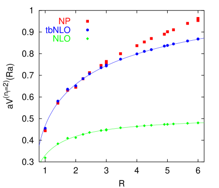
Figure 38: The non-perturbative potential for Wilson fermions at $\beta=5.6$, $\kappa=0.1565$, i.e. $ma\approx 0.04$, in comparison with NLO tadpole improved boosted and bare perturbation theory.

In Fig. 38 we compare the NP $n_{f}=2$ potential with NLO and tbNLO perturbation theory. In the latter case we used the value $\Lambda_{\overline{MS}}r_{0}=0.570(6)$, as obtained from the plaquette $\Box=0.57073$. The situation is very similar to that of the quenched potential at $\beta=6.0$ depicted in Figs. 32 and 33 which is why we refrain from including LO, bLO, bNLO and tbLO curves. The respective NNLO results are not known at present, even at large $R$.

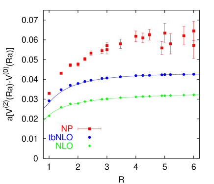
Figure 39: The difference between the $n_{f}=2$ lattice potential with Wilson fermions at $\beta=5.6$, $\kappa=0.1565$ and the quenched potential at $\beta=6.0$: non-perturbatively vs. perturbatively.

In a next step we calculate the difference between the $n_{f}=2$ and the $n_{f}=0$ potentials. This is depicted in Fig. 39, together with the respective differences calculated in tbNLO and NLO. The NP linear confining term cancels in this combination, such that there is some reason to believe that this difference should be more perturbative than the potentials themselves, at least as long as $R<12$, the distance at which the QCD string will eventually “break” in the $n_{f}=2$ case. In the NP as well as perturbative data sets lattice artefacts are clearly visible that can be ascribed to the effect of the sea quarks. In the case of NLO we have depicted the $n_{f}=0$ expectation using the slightly smaller one loop matched value $\beta=5.969$ rather than $\beta=6.0$ for internal consistency.

As $R\rightarrow\infty$ all three curves approach constant values as the massive fermions start to decouple from the running. Although the shape of all curves is similar, even the tbNLO prediction underestimates the NP data by almost 30 %. This is not surprising as the vertical scale has been vastly inflated after subtracting two quantities of similar size from each other. For instance we can almost completely eliminate the gap between the NP and tbNLO results by increasing the $\Lambda_{\overline{MS}}^{(2)}r_{0}$ value (or decreasing the $\Lambda_{\overline{MS}}^{(0)}r_{0}$ value) by only 3 %. We find it quite encouraging that at least on a qualitative level we are able to resolve sea quark effects that only appear from ${\mathcal{O}}(\alpha^{2})$ onwards in perturbation theory. Unsurprisingly, a quantitative understanding is not possible without knowledge of the difference to second non-trivial order, i.e. ${\mathcal{O}}(\alpha^{3})$ in this case.

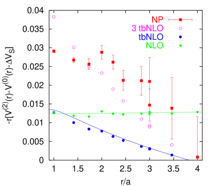
Figure 40: The same as Fig. 39 but with the difference of the respective self energy contributions subtracted, and multiplied by $-r$. We estimate $a\Delta V_{S}^{\mbox{\scriptsize NP}}\approx 0.062$ and find $a\Delta V_{S}^{\mbox{\scriptsize tbNLO}}\approx 0.042$ and $a\Delta V_{S}^{\mbox{\scriptsize NLO}}\approx 0.034$. “3 tbNLO” refers to the tbNLO result, multiplied by three.

We now turn to the difference in the running of the two respective Coulomb couplings, between $n_{f}=2$ and $n_{f}=0$ and depict the quantity $\Delta e(R)=-Ra[V^{(2)}(Ra)-V^{(0)}(Ra)-\Delta V_{S}]$ in Fig. 40. This combination further inflates scale and errors, in particular at large $R$. In the tbNLO case we can now identify deviations between the curve that constitutes the large $R$ limit and the points calculated in lattice perturbation theory at short distances. This bias, which also appeared in Fig. 16 and which turns out to be an ${\mathcal{O}}(ma)$ lattice artefact, has been discussed in Sec. III.3 above. Since at this lattice spacing, and within the scale of the figure, perturbative predictions and NP data cannot be expected to agree with each other anymore (cf. Fig. 39) we subtract different $\Delta V_{S}$ values from the three data sets. While we compute $a\Delta V_{S}^{\mbox{\scriptsize NLO}}$ and $a\Delta V_{S}^{\mbox{\scriptsize tbNLO}}$ in perturbation theory, we fit $a\Delta V_{S}^{\mbox{\scriptsize NP}}\approx 0.062$ from the NP data depicted in Fig. 39.

The NP data indicates an enhancement of the Coulomb coupling in the $n_{f}=2$ case at the given mass by almost 0.03 over the quenched coupling at short distances. This enhancement then reduces to zero at large distances where the two data sets are matched. Contrary to this we find the bare NLO expectation to be rather flat as a function of $R$: the running of the coupling with $R$ is faster when fermions are included, however, this effect is compensated for by a larger value of $g^{2}$, in comparison with the quenched case. This larger bare coupling can be translated into a deflation of the distance scale which in turn slows down the running again. In the end one would expect an increase of $e$ by 0.012 – 0.013 to NLO. The tbNLO prediction includes some slope but falls short of the NP data by a factor of about 3. After multiplying the points by this factor (open circles) the agreement with the NP $\Delta e(R)$ is at best qualitative. We should not forget however that in the figure we have vastly inflated tiny differences. Unfortunately, $n_{f}=2$ lattice simulations at finer lattice spacings are not yet available such that we cannot test to what extent the quality of the parametrization improves as the continuum limit is approached.

V Summary

We have calculated Wilson loops, the static potential and the static source self energy to ${\mathcal{O}}(\alpha^{2})$ in lattice perturbation theory with the Wilson gluonic action as well as with massive Wilson-Sheikholoslami-Wohlert and Kogut-Susskind fermions for arbitrary representation of the external sources. Some numbers for “improved” gluonic actions are provided too. The results are useful for understanding violations of rotational symmetry and the effect of including sea quarks on the lattice. Lattice results can be related to other regularization schemes like the perturbatively defined $\overline{MS}$ scheme, for instance to allow for an extraction of the QCD coupling at high energies from low energy hadronic phenomenology.

We find that at presently employed quark masses lattice spacing effects on the short distance potential are not smaller in absolute terms for the two non-perturbatively ${\mathcal{O}}(a)$ improved fermionic actions, relative to the Wilson action. However, improvement results in a reduced mass dependence around $ma=0$ of quantities like the static source self energy, that is required for determinations of the $b$ quark mass in an effective field theory framework, small Wilson loops and in the matching between lattice and $\overline{MS}$ schemes at finite $a$.

We perturbatively determined $\beta=2N/g^{2}$ shifts between the pure gauge theory and QCD with massive sea quarks. The results appear to be reliable within 10 % for quark masses down to 20 MeV for Wilson type fermions (which translates into less than 1 % uncertainty in the value of the predicted matched $\beta$) and within 25 % for “$n_{f}=2$” KS fermions within a window of lattice spacings that correspond to quenched $\beta$ values $5.8<\beta<6.15$. This method might turn out to be useful in predicting the impact of a shift in the sea quark mass onto correlation lengths like $r_{0}/a$ in future simulations. In particular we confirm that for SW fermions the lines of constant $r_{0}/a$ and $m_{\pi}a$ are significantly tilted with respect to those of constant $\beta$ and $ma$, respectively, a fact that complicates continuum limit extrapolations.

The success of the perturbative matching of the running coupling at flavour thresholds via an intermediate mass-dependent scheme, in our case the potential scheme, in lattice simulations (which allow us to compare with the correct non-perturbative result) means that the standard procedures employed in perturbative calculations Bernreuther:1983zp ; Brodsky:1998mf should be quite reliable even at the charm quark mass.

We investigated so-called boosted perturbation theory methods Parisi:1980pe ; lepage and found them to work well in many cases. However, such methods have to be digested with some caution: as boosted ${\mathcal{O}}(\alpha^{2})$ perturbation theory is tuned to reduce higher order and in particular ${\mathcal{O}}(\alpha^{3})$ corrections, differences between results calculated at these two orders are not necessarily indicative of the systematic uncertainties involved. In the absence of even higher order calculations, the perturbative uncertainty in for instance predictions of the running coupling can be estimated by varying both, the quantity from which the coupling is determined and the lattice spacing $a$.

In analysing quenched lattice data on the static potential and plaquette we obtain the value $\Lambda_{\overline{MS}}^{(0)}r_{0}=0.61(9)$ which is in agreement with $\Lambda_{\overline{MS}}^{(0)}r_{0}=0.60(5)$ obtained by use of finite size techniques by the ALPHA Collaboration Bode:1999hd . The error which is dominated by the uncertainty of higher order perturbative corrections can be systematically reduced by an ${\mathcal{O}}(\alpha^{3})$ calculation of the static potential. Using Wilson, KS and SW $n_{f}=2$ lattice data, the latter with Wilson as well as with Iwasaki glue, we estimate $\Lambda_{\overline{MS}}^{(2)}r_{0}=0.69(15)$ in the continuum and chiral limit, where the error is again dominated by systematics. We find this value to depend strongly on both, the quark mass and the lattice spacing. Chiral and in particular continuum limit extrapolations are not fully under control but the use of different input quantities and lattice actions allows us to estimate the systematic uncertainties.

Based on the $n_{f}=0$ and $n_{f}=2$ estimates we guess $\Lambda_{\overline{MS}}^{(3)}=270(70)$ MeV. This value corresponds to $\alpha_{\overline{MS}}^{(5)}(m_{Z})=0.1133(59)$. In spite of the fact that more lattice data entered our analysis than has been used in any of the previous attempts to determine the $n_{f}=2$ running coupling, our error estimate is not smaller but larger than those that have been quoted by various lattice groups in the past El-Khadra:1992vn ; davi1 ; davi2 ; Spitz:1999tu ; Marcantonio:2001fc ; Booth:2001qp ; davi3 . The main reason is that the use of different quark actions and observables for the first time enabled us to realistically assess the uncertainties connected to higher order perturbative corrections and chiral and continuum extrapolations.

We estimate that the error on the QCD coupling at the $Z$ boson mass can be reduced to about 4 %, once a set of $n_{f}=2+1$ lattice simulations, similar to those that are already available for $n_{f}=2$, becomes available. By improving the perturbative calculation to NNLO as well as by incorporating a wider range of lattice spacings into the numerical simulations, errors of 1 – 2 % appear to be realistic within the next few years. It might be possible to further improve on this quality by a dedicated lattice simulation of running quark masses and coupling DellaMorte:2002vm .

We found that the lattice potential at distances smaller than about 1 GeV^-1 is quite well described by NLO boosted tadpole improved perturbation theory without any free parameter, as long as no attempt is made to subtract the power divergent static self energy. This observation is somewhat in contrast to previous beliefs Bali:1999ai ; Necco:2001gh and supports the view that perturbation theory for this quantity (and not only for the force) might be quite reliable in the continuum too. This is so as long as renormalons (in the ${\overline{MS}}$ scheme) and power divergences (in the lattice scheme) are properly dealt with when rearranging the perturbative series Pineda:2002se ; sumino . At distances larger than 1 GeV^-1 the linear confining term sets in rather rapidly and it is doubtful that this behaviour can be emulated completely by higher order perturbative corrections. At distances shorter than 1 GeV^-1 the difference between non-perturbative data and perturbative expectation is dominated by a quadratic term with a coefficient of ${\mathcal{O}}(1)$ in units of $\Lambda_{\overline{MS}}$. The dependence of this coefficient on the way in which the perturbative series is organized, on the $\Lambda_{\overline{MS}}r_{0}$ value that is used and on the lattice spacing deserves further study.

It turned out to be possible to resolve the difference in the logarithmic running of the coupling between two flavour QCD and the quenched approximation from non-perturbative data on the static potential. This difference is in rough qualitative agreement with the NLO expectation, however, about three times larger than expected. Unfortunately, at present we are limited to inverse lattice spacings of 2 GeV such that it is not possible to judge whether the discrepancy reduces as the scale is increased. As the magnitude of the effect should also increase as the quark mass is reduced, next generation lattice data at smaller quark masses should turn out helpful too.

Appendix A Perturbative relations between lattice and continuum schemes

We review the known perturbative relations between the lattice $\beta$-function and the modified minimal subtraction $(\overline{MS})$ scheme for various lattice actions in $SU(N)$ gauge theory with $n_{f}$ fermion flavours. We also display continuum perturbation theory results for the (mass dependent) static potential in position space, which constitute the limit against which our calculations will converge for $r\gg a$.

A.1 Conventions

We define the QCD $\beta$-function as,

$$\beta(\alpha)=\frac{d\alpha}{d\ln\mu^{2}}=-\beta_{0}\alpha^{2}-\beta_{1}\alpha^{3}-\beta_{2}\alpha^{4}-\cdots.$$ (121)

While in mass-independent schemes like lattice regularization or minimal subtraction the first two coefficients,

$$\beta_{0} = \left(\frac{11}{3}N-\frac{2}{3}n_{f}\right)\frac{1}{4\pi},$$ (122)

$$\beta_{1} = \left[\frac{34}{3}N^{2}-\left(\frac{13}{3}N-\frac{1}{N}\right)n_{f}\right]\frac{1}{(4\pi)^{2}},$$ (123)

are universal, $\beta_{2}$ will in general depend on the renormalization scheme. In the $\overline{MS}$ scheme $\beta_{2}$ reads Tarasov:1980au ,

$$\beta_{2}^{\overline{MS}} = \left[\frac{2857}{54}N^{3}-\left(\frac{1709}{54}N^{2}-\frac{187}{36}-\frac{1}{4N^{2}}\right)n_{f}\right.$$ (124)

$$+\left.\left(\frac{56}{27}N-\frac{11}{18N}\right)n_{f}^{2}\right]\frac{1}{(4\pi)^{3}}.$$

The QCD $\Lambda$-parameter in a given scheme is defined as,

$$\Lambda=\lim_{\mu\rightarrow\infty}\mu\,\exp\left(-\frac{1}{2\beta_{0}\alpha(\mu)}\right)\left[\beta_{0}\alpha(\mu)\right]^{-\frac{\beta_{1}}{2\beta_{0}^{2}}}.$$ (125)

We discuss the conversion between two different renormalization schemes: let,

$$\alpha^{\prime}(\mu)=\alpha(\mu)+c_{1}\alpha^{2}(\mu)+c_{2}\alpha^{3}(\mu)+\cdots.$$ (126)

From the definition of the $\beta$-function, Eq. (121), one infers,

$$\beta_{0}^{\prime} = \beta_{0},\quad\beta_{1}^{\prime}=\beta_{1},$$ (127)

$$\beta_{2}^{\prime} = \beta_{2}-c_{1}\beta_{1}+(c_{2}-c_{1}^{2})\beta_{0},$$ (128)

$$\Lambda^{\prime} = \Lambda\,e^{c_{1}/(2\beta_{0})}.$$ (129)

If not only the scheme but also the matching scale $\mu$ is shifted, one easily obtains the relation,

$$\alpha^{\prime}(\mu^{\prime})=\alpha(\mu)+c_{1}^{\prime}\alpha^{2}(\mu)+c_{2}^{\prime}\alpha^{3}(\mu)+\cdots,$$ (130)

with,

$$c_{1}^{\prime} = c_{1}-2\beta_{0}\ln\left(\frac{\mu^{\prime}}{\mu}\right),$$ (131)

$$c_{2}^{\prime} = c_{2}-\left(2\beta_{1}+4c_{1}\beta_{0}\right)\ln\left(\frac{\mu^{\prime}}{\mu}\right)$$

$$+4\beta_{0}^{2}\ln^{2}\left(\frac{\mu^{\prime}}{\mu}\right)$$

$$= c_{2}-2\beta_{1}\ln\left(\frac{\mu^{\prime}}{\mu}\right)+{c_{1}^{\prime}}^{2}-c_{1}^{2}.$$

A.2 Conversion between the $\overline{MS}$ and lattice schemes

The $\overline{MS}$ coupling is related to the lattice coupling $\alpha_{L}=g^{2}/(4\pi)$ via,

$$\alpha_{\overline{MS}}(a^{-1})=\alpha_{L}+b_{1}\alpha_{L}^{2}+b_{2}\alpha^{3}+\cdots,$$ (133)

where for the Wilson and Sheikholeslami-Wohlert (SW) quark actions one obtains Hasenfratz:1980kn ; Weisz:1981pu ; Luscher:1995np ; Alles:1998is ; Christou:1998ws ,

$$b_{1}=-\frac{\pi}{2N}+k_{1}N+K_{1}(ma)n_{f},$$ (134)

where $K_{1}(ma)=K_{1}(0)+\Delta K_{1}(ma)$, with the numerical values,

$$k_{1} = 2.135730074078457(2),$$ (135)

$$K_{1}(0) = -0.08414443(6)$$

$$+0.0634188788(1)c_{SW}$$

$$-0.3750240693(1)c_{SW}^{2},$$

for the Wilson parameter $r=1$. The tree-level value of the SW coefficient, $c_{SW}=1+3.3414(9)\alpha_{L}+\cdots=c_{SW}^{(0)}+c_{SW}^{(1)}g^{2}+\cdots$, is $c_{SW}^{(0)}=1$. In the case of Kogut-Susskind (KS) fermions $K_{1}(0)$ reads Weisz:1981pu ; Luscher:1995zz ,

$$K^{KS}_{1}(0)=-0.03298341916(1).$$ (137)

Note that in our notation $n_{f}$ KS quark flavours correspond to $n_{f}$ (not $4\,n_{f}$) flavours of Dirac quarks in the continuum limit. Therefore, $n_{f}$ has to be a multiple of four. The value of $k_{1}$ applies to the Wilson gluonic action only. However, the contribution $K_{1}(ma)$ (whose quark mass dependence has been calculated for the first time in this publication and is displayed in Tab. 10) remains the same for Symanzik type improvements of the Wilson gluonic action.

At vanishing quark mass or lattice spacing, $m\ll a^{-1}$ we obtain the massless limit, i.e. $\Delta K_{1}(0)=0$. The mass dependent term results in a change of the QCD $\beta$-function at finite $a$:

$$\beta_{0}^{L}=\beta_{0}^{\overline{MS}}-\sum_{i}\frac{a}{2}\frac{d\Delta K_{1}(m_{i}a)}{da}.$$ (138)

From this we can infer, $\lim_{ma\rightarrow 0}d\Delta K_{1}(ma)/d\ln a=\lim_{ma\rightarrow 0}d\Delta K_{1}(ma)/d\ln(am)=0$: the dependence is regular in $ma$ near the origin. Since the $\beta$-function is no on-shell quantity, we cannot exclude terms proportional to $ma$, even for improved quark actions. By demanding that in the limit $ma\rightarrow\infty$ the quenched $\beta$-function is re-obtained, we find,

$$\lim_{x\rightarrow\infty}\frac{d\Delta K_{1}(x)}{d\ln x}=-\frac{1}{3\pi},$$ (139)

i.e. $-\Delta K_{1}$ will grow logarithmically for large $ma$. This is expected since $ma\rightarrow\infty$ means that the coupling on the left hand side of Eq. (133) runs with $n_{f}$ active flavours while the running on the lattice side of this equation corresponds to that of pure Yang-Mills theory. The difference has to be compensated for by $\Delta K_{1}(ma)$. We will determine the integration constant in the region $ma\rightarrow\infty$ in Eq. (B.2) below from matching the un-quenched and quenched static potentials in the infra red.

The coefficient $b_{2}$ is at present only known for massless Wilson-SW quarks and Wilson gluonic action:

$$b_{2}=b_{1}^{2}+\frac{3\pi^{2}}{8N^{2}}+k_{2}+k_{3}N^{2}+\left(\frac{K_{2}}{N}+K_{3}N\right)n_{f}$$ (140)

with Christou:1998ws ; Bode:2001uz

$$k_{2} = -2.8626215972(6),$$ (141)

$$k_{3} = 1.24911585(3),$$ (142)

$$K_{2} = 0.1890(2)$$

$$-0.02492(5)c_{SW}-0.83585(3)c_{SW}^{2}$$

$$-0.79942(5)c_{SW}^{3}-0.012947(2)c_{SW}^{4},$$

$$K_{3} = -0.1579(3)$$

$$-0.00540(6)c_{SW}+0.7684(1)c_{SW}^{2}$$

$$+0.033842(5)c_{SW}^{3}+0.006920(2)c_{SW}^{4}.$$

From Eqs. (128) and (129) we infer,

$$\beta_{2}^{L} = \beta_{2}^{\overline{MS}}+b_{1}\beta_{1}-(b_{2}-b_{1}^{2})\beta_{0},$$ (145)

$$\Lambda_{\overline{MS}} = \Lambda_{L}\exp\left(\frac{b_{1}}{2\beta_{0}}\right).$$ (146)

This results for instance in the numerical values,

$$\Lambda^{(0)}_{\overline{MS}} \approx 28.809\,\Lambda_{L}^{(0)},$$ (147)

$$\Lambda^{(2)}_{\overline{MS}} \approx 41.053\,\Lambda_{L}^{W,(2)}\approx 27.379\,\Lambda_{L}^{SW,(2)},$$ (148)

for $N=3$ colours.

A.3 Conversion between the $\overline{MS}$ scheme and schemes based on the static potential

We define the coupling $\alpha_{V}$ through the static QCD potential in momentum space,

$$\tilde{V}(q)=-4\pi C_{F}\frac{\alpha_{V}(q)}{q^{2}},$$ (149)

where $q=|{\mathbf{q}}|$ and $C_{F}=(N^{2}-1)/(2N)$. The momentum space potential is related to that in position space via a Fourier transformation,

$$\tilde{V}(q)=\int\frac{d^{3}x}{(2\pi)^{3}}[V(r)-V_{S}]e^{i{\mathbf{q}}{\mathbf{x}}},$$ (150)

where $r=|{\mathbf{x}}|$. $V_{S}$ denotes the self energy term, that vanishes in dimensional regularization but will in general be present, and the position space potential,

$$V(r)=-C_{F}\frac{\alpha_{R}(r^{-1})}{r}+V_{S},$$ (151)

defines the coupling $\alpha_{R}$. By Fourier transformation one obtains the relation between the two schemes,

$$\alpha_{R}(\mu)=\alpha_{V}\left(e^{-\gamma}\mu\right)\left(1+\frac{\pi^{2}\beta_{0}^{2}}{3}\alpha^{2}\right),$$ (152)

which holds for fermion masses $m_{i}\ll\mu$. $\gamma=0.57721566\ldots$ is the Euler constant.

We write,

$$\alpha_{V}(\mu)=\alpha_{\overline{MS}}(\mu)+a_{1}\alpha_{\overline{MS}}^{2}(\mu)+a_{2}\alpha^{3}+\cdots.$$ (153)

The coefficients $a_{1}$ and $a_{2}$ are known. For $n_{f}$ massless quark flavours they read Schroder:1999vy :

$$a_{1} = \left(\frac{31}{9}N-\frac{10}{9}n_{f}\right)\frac{1}{4\pi},$$ (154)

$$a_{2} = \left\{\left(\frac{4343}{162}+4\pi^{2}-\frac{\pi^{4}}{4}+\frac{22}{3}\zeta_{3}\right)N^{2}\right.$$ (155)

$$- \left[\left(\frac{1798}{81}+\frac{56}{3}\zeta_{3}\right)\frac{N}{2}+\left(\frac{55}{3}-16\zeta_{3}\right)\frac{C_{F}}{2}\right]n_{f}$$

$$+ \left.\frac{100}{81}n_{f}^{2}\right\}\frac{1}{16\pi^{2}}.$$

$\zeta_{3}$ denotes the value of the $\zeta$-function $\zeta(3)=1.20205690\ldots$. The corresponding result for massive quark flavours with masses $m_{i}$ has been obtained in Ref. Melles:2000dq :

$$a_{1}(\{m_{i}\}) = a_{1}+\frac{1}{6\pi}\sum_{i=1}^{n_{f}}\ln\left(1+\frac{C_{0}m_{i}^{2}}{\mu^{2}}\right),$$ (156)

$$a_{2}(\{m_{i}\}) = a_{2}+\frac{19}{48\pi^{2}}\sum_{i=1}^{n_{f}}\left\{\ln\left(1+\frac{C_{3}}{C_{2}}\frac{m_{i}^{2}}{\mu^{2}}+\frac{1}{C_{2}}\frac{m_{i}^{4}}{\mu^{4}}\right)\right.$$

$$+\left.\frac{C_{3}-2C_{1}}{\sqrt{C_{3}^{2}-4C_{2}}}\left\{2\ln\left(1+\frac{C_{3}+\sqrt{C_{3}^{2}-4C_{2}}}{2C_{2}}\frac{m_{i}^{2}}{\mu^{2}}\right)-\ln\left[1+\left(2+\frac{C_{3}}{C_{2}}\right)\frac{m_{i}^{2}}{\mu^{2}}\right]\right\}\right\}$$

$$+\frac{1}{54\pi^{2}}\sum_{i=1}^{n_{f}}\left(\frac{31}{2}N-5n_{f}\right)\ln\left(1+\frac{C_{0}m_{i}^{2}}{\mu^{2}}\right)+\frac{1}{36\pi^{2}}\sum_{i,j=1}^{n_{f}}\ln\left(1+\frac{C_{0}m_{i}^{2}}{\mu^{2}}\right)\ln\left(1+\frac{C_{0}m_{j}^{2}}{\mu^{2}}\right),$$

with the numerical values Brodsky:1999fr ,

$$C_{0} = 5.19(3),$$ (158)

$$C_{1} = -0.571(34),$$ (159)

$$C_{2} = 0.221(15),$$ (160)

$$C_{3} = 1.33(12).$$ (161)

A change in the argument on the left hand side of Eq. (153), $\alpha_{V}(\mu)\mapsto\alpha_{V}(\mu^{\prime})$, results in the substitutions,

$$a_{1}(\mu^{\prime},\{m_{i}\}) = a_{1}\left(\left\{m_{i}\frac{\mu}{\mu^{\prime}}\right\}\right)-2\beta_{0}\ln\left(\frac{\mu^{\prime}}{\mu}\right),$$ (162)

$$a_{2}(\mu^{\prime},\{m_{i}\}) = a_{2}\left(\left\{m_{i}\frac{\mu}{\mu^{\prime}}\right\}\right)+4\beta_{0}^{2}\ln^{2}\left(\frac{\mu^{\prime}}{\mu}\right)$$

$$-\left[2\beta_{1}+4\beta_{0}a_{1}\left(\left\{m_{i}\frac{\mu}{\mu^{\prime}}\right\}\right)\right]\ln\left(\frac{\mu^{\prime}}{\mu}\right),$$

in analogy to Eqs. (131) – (A.1).

The masses $m_{i}$ in Eqs. (156) – (A.3) denote pole masses,

$$m=\left[1+\frac{C_{F}}{4\pi}\left(4-3\ln\frac{m^{2}}{\mu^{2}}\right)\alpha\right]m_{\overline{MS}}(\mu).$$ (164)

Re-expressing Eq. (A.3) in terms of $\overline{MS}$ quark masses $m_{i}$ at a scale $\mu$, therefore, results in the replacement,

$$a_{2}^{\overline{MS}}(\{m_{i}\})=a_{2}(\{m_{i}\})+\frac{C_{F}}{12\pi^{2}}\sum_{i=1}^{n_{f}}\frac{4-3\ln\frac{m_{i}^{2}}{\mu^{2}}}{1+\frac{\mu^{2}}{C_{0}m_{i}^{2}}},$$ (165)

while Eq. (156) remains unaffected. For Wilson fermions one obtains Capitani:2001xi ,

$$m_{\overline{MS}}(a^{-1})=\left(1+16.95241\frac{C_{F}}{4\pi}\alpha\right)m_{0}.$$ (166)

Hence, in terms of lattice quark masses $m_{i}(a)$, $a_{2}$ reads:

$$a_{2}^{L}(\{m_{i}\})=a_{2}(\{m_{i}\})+\frac{C_{F}}{12\pi^{2}}\sum_{i=1}^{n_{f}}\frac{16.95241-3\ln m_{i}^{2}a^{2}}{1+\left(C_{0}m_{i}^{2}a^{2}\right)^{-1}}.$$ (167)

We now go to position space and write,

$$\alpha_{R}(\mu)=\alpha_{\overline{MS}}(\mu)+a_{1}^{R}\alpha_{\overline{MS}}^{2}(\mu)+a_{2}^{R}\alpha^{3}+\cdots.$$ (168)

In following Eqs. (130) – (A.1) we obtain from Eqs. (152) and (153),

$$a_{1}^{R} = a_{1}+2\gamma\beta_{0},$$ (169)

$$a_{2}^{R} = a_{2}+4\gamma\beta_{0}a_{1}+2\gamma\beta_{1}+\left(4\gamma^{2}+\frac{\pi^{2}}{3}\right)\beta_{0}^{2}.$$ (170)

The one loop result for massive quark flavours reads,

$$a_{1}^{R}(\{m_{i}\})=a_{1}^{R}+\frac{1}{3\pi}\sum_{i=1}^{n_{f}}\mbox{Ein}\left(\frac{\sqrt{C_{0}}m_{i}}{\mu}\right)$$ (171)

with

$$\mbox{Ein}(x)=\gamma+\ln(x)+E_{1}(x)=-\sum_{\nu=1}^{\infty}\frac{(-x)^{\nu}}{\nu\,\nu!}.$$ (172)

For the corresponding two-loop mass dependence of the position space potential we refer to Ref. Melles:2000dq . The exponential integral $E_{1}(x)$ is defined by,

$$E_{1}(x)=\int_{x}^{\infty}dt\frac{e^{-t}}{t},$$ (173)

i.e.

$$\mbox{Ein}(x)=\int_{0}^{x}dt\frac{1-e^{-t}}{t}.$$ (174)

From Eqs. (126), (129), (153) and (154) one obtains the numerical values,

$$\Lambda_{V}^{(0)}\approx 1.5995\,\Lambda_{\overline{MS}}^{(0)},\quad\Lambda_{V}^{(2)}\approx 1.5213\,\Lambda_{\overline{MS}}^{(2)},$$ (175)

while Eq. (152) results in,

$$\Lambda_{R}^{(n_{f})}=e^{\gamma}\Lambda_{V}^{(n_{f})}\approx 1.7811\,\Lambda_{V}^{(n_{f})}.$$ (176)

Note that for massive quarks the coefficients of the $V$- and $R$-scheme $\beta$-functions become explicitly scale dependent. However, this does not affect the respective QCD $\Lambda$-parameters, that are defined in the limit $\mu\rightarrow\infty$ [Eq. (125)].

We obtain:

$$\frac{d\alpha_{V}}{d\ln\mu^{2}}=-\left[\beta_{0}^{(n_{f})}+\frac{1}{6\pi}\sum_{i=1}^{n_{f}}\left(1+\frac{\mu^{2}}{C_{0}m_{i}^{2}}\right)^{-1}\right]\alpha_{V}^{2}(\mu)+\cdots$$ (177)

$$\frac{d\alpha_{R}}{d\ln\mu^{2}}=-\left\{\beta_{0}^{(n_{f})}+\frac{1}{6\pi}\sum_{i=1}^{n_{f}}\left[1-\exp\left(-\frac{\sqrt{C_{0}}m_{i}}{\mu}\right)\right]\right\}\alpha_{R}^{2}(\mu)+\cdots.$$ (178)

In the situation, $m_{1}=m_{2}=\cdots=m_{n_{f}-1}=0,m_{n_{f}}>0$, the above coefficient functions smoothly interpolate between $\beta_{0}^{(n_{f}-1)}$ (for $\mu/m_{n_{f}}\rightarrow 0$) and $\beta_{0}^{(n_{f})}$ (for $\mu/m_{n_{f}}\rightarrow\infty$) as one would expect.

A.4 The perturbative potential at large $R$.

We denote a dimensionless distance measured in lattice units by $R$ while $r=Ra$ refers to the distance in physical units. At separations $R\gg 1$, i.e. $r\gg a$, rotational invariance should be restored and the static potential obtained in lattice perturbation theory should coincide with the one computed above by use of dimensional regularization. In the large $R$ limit our results should therefore approach the continuum expressions given in Appendix A.3 above.

We define,

$$aV({\mathbf{R}}a) = v_{1}({\mathbf{R}})\alpha_{L}+v_{2}({\mathbf{R}})\alpha_{L}^{2}+\cdots,$$ (179)

$$aV_{S} = v_{1}(\infty)\alpha_{L}+v_{2}(\infty)\alpha_{L}^{2}+\cdots,$$ (180)

where the self-energy $V_{S}=2\delta m_{\mbox{\scriptsize stat}}$ is twice the lattice pole mass of a static colour source. The coefficient functions $v_{i}({\mathbf{R}})$ have been calculated in the present article. At large separations we expect $v_{i}({\mathbf{R}})$ only to depend on the modulus $R=|{\mathbf{R}}|$ and can write,

$$v_{c,i}(R)=v_{i}(R)-v_{i}(\infty).$$ (181)

Eq. (151) now implies,

$$a\left[V({\mathbf{R}}a)-V_{S}\right]\longrightarrow-C_{F}\frac{\alpha_{R}\left[(Ra)^{-1}\right]}{R}\quad(R\rightarrow\infty).$$ (182)

It follows,

$$v_{1}({\mathbf{R}})-v_{1}(\infty)\longrightarrow v_{c,1}(R)=-\frac{C_{F}}{R}\quad(R\rightarrow\infty),$$ (183)

where

$$v_{1}(\infty)=C_{F}\times 3.1759115\ldots,$$ (184)

for the Wilson gluonic action. $v_{2}(\infty)$ is also known. Here we state the result for massless Wilson-SW quark flavours and $N=3$:

$$v_{2}(\infty) = C_{F}\times\{16.714(4)+[-0.42333(6)$$

$$+0.0516(2)c_{SW}-0.5870(2)c_{SW}^{2}]n_{f}\}.$$

In the case of massless KS quarks the numerical value of the $n_{f}$ coefficient is $-C_{F}\times 0.36846(6)$. Results on the mass dependence of the fermionic coefficients can be found in Tabs. 12 and 13. The $n_{f}=0$ result has first been derived in Refs. Weisz:1984bn ; Heller:1985hx . The precision has subsequently been increased by Martinelli and Sachrajda Martinelli:1999vt . We do, however, slightly disagree with this reference and obtain $\delta m_{\mbox{\scriptsize stat},2}=C_{F}v_{2}(\infty)/2=11.143(3)$, rather than 11.152 Martinelli:1999vt . The latter reference includes the Wilson and SW contributions for massless fermions as well, which we were able to reproduce with increased precision. The mass dependence of $v_{2}(\infty)$ as well as the KS result are new. The $n_{f}=0$ value for $v_{3}(\infty)$ has recently been obtained by means of stochastic perturbation theory DiRenzo:2001nd :

$$v_{3}(\infty)=C_{F}\times 129(2).$$ (186)

This result agrees with the one of Ref. Trottier:2001vj $v_{3}(\infty)=C_{F}\times 130(1)$, obtained from a fit to high $\beta$ Monte Carlo data.

From Eqs. (179) – (183) we obtain,

$$\alpha_{R}\left[(Ra)^{-1}\right]=\alpha_{L}+e_{1}(R)\alpha_{L}^{2}+e_{2}(R)\alpha_{L}^{3}+\cdots$$ (187)

with

$$e_{i}(R)=\frac{v_{c,i+1}(R)}{v_{c,1}(R)}=-\frac{R}{C_{F}}v_{c,i+1}(R).$$ (188)

In converting the scheme and scale by use of Eqs. (168), (133) and (130) – (A.1), we obtain the coefficients $e_{1}(R)$ and $e_{2}(R)$:

$$\alpha_{R}\left[(Ra)^{-1}\right] = \alpha_{\overline{MS}}[(Ra)^{-1}]+a_{1}^{R}(\{Rm_{i}\})\alpha_{\overline{MS}}^{2}[(Ra)^{-1}]+a_{2}^{R}(\{Rm_{i}\})\alpha^{3}$$ (189)

$$= \alpha_{L}+\left[b_{1}+a_{1}^{R}(\{Rm_{i}\})+2\beta_{0}\ln R\right]\alpha_{L}^{2}+\left\{b_{2}+a_{2}^{R}(\{Rm_{i}\})+2b_{1}a_{1}^{R}(\{Rm_{i}\})\right.$$

$$+ \left.[2\beta_{1}+4(b_{1}+a_{1}^{R}(\{Rm_{i}\}))\beta_{0}]\ln R+4\beta_{0}^{2}\ln^{2}R\right\}\alpha^{3}.$$

Therefore,

$$v_{c,2}(R) = -\frac{C_{F}}{R}\left[b_{1}+a_{1}^{R}(\{Rm_{i}\})+2\beta_{0}\ln R\right],$$ (190)

$$v_{c,3}(R) = -\frac{C_{F}}{R}\left\{b_{2}+a_{2}^{R}(\{Rm_{i}\})+2b_{1}a_{1}^{R}(\{Rm_{i}\})+[2\beta_{1}+4(b_{1}+a_{1}^{R}(\{Rm_{i}\}))\beta_{0}]\ln R+4\beta_{0}^{2}\ln^{2}R\right\}.$$ (191)

This amounts to

$$v_{c,2}(R)=-\frac{C_{F}}{R}\left\{A_{0}+A_{1}\ln R+\sum_{i=1}^{n_{f}}\left[\Delta K_{1}(m_{i}a)+\frac{1}{3\pi}\mbox{Ein}(\sqrt{C_{0}}m_{i}aR)\right]\right\}$$ (192)

with the numerical values for $n_{f}$ flavours of Wilson-SW fermions in $SU(3)$ QCD,

$$A_{0} \approx 7.7164259753$$

$$- [0.233808-0.063419(1)c_{SW}+0.37524(1)c_{SW}^{2}]n_{f},$$

$$A_{1} \approx 1.75070437401-0.10610329540\,n_{f}.$$ (194)

For KS fermions the fermionic contribution to $A_{0}$ differs:

$$A_{0}^{KS}\approx 7.7164259753-0.1826473162\,n_{f}.$$ (195)

The function $\mbox{Ein}(x)$ is defined in Eq. (172) and can be approximated for small arguments by,

$$\frac{1}{R}\mbox{Ein}\left(\sqrt{C_{0}}m_{i}aR\right)=\sqrt{C_{0}}m_{i}a+{\mathcal{O}}\left[(m_{i}aR)^{2}\right]:$$ (196)

to leading order the coefficient $v_{c,2}(R)$ is parallel shifted in proportion to $ma$ at short distances.

At infra red scales, $Ra\gg m_{i}^{-1}$, $E_{1}(x)\propto e^{-x}/x$, such that the massive flavours decouple from the logarithmic running of the potential. For $n_{f}$ massive degenerate flavours with masses $m_{i}=m$, we find:

$$v_{c,2}^{(n_{f})}(R) \stackrel{{\scriptstyle R\rightarrow\infty}}{{\longrightarrow}}v_{c,2}^{(0)}(R)$$

$$-\frac{n_{f}C_{F}}{R}\left\{K_{1}(ma)+\frac{1}{3\pi}\left[\ln\left(\sqrt{C_{0}}ma\right)-\frac{5}{6}\right]\right\}.$$

For massless fermions we can parametrize the next order term in the expansion of the lattice potential $v_{c,3}$ by [Eq. (191)],

$$v_{c,3}=-\frac{C_{F}}{R}\left(B_{0}+B_{1}\ln R+B_{2}\ln^{2}R\right).$$ (198)

The fermionic part of $b_{2}$, which is required to calculate the contribution to $B_{0}$ that is proportional to $n_{f}$, is only known for massless Wilson-SW fermions. Restricting ourselves to massless Wilson quarks and $SU(3)$ we obtain the numerical values,

$$B_{0}\approx 73.8166085803$$

$$-3.667(1)\,n_{f}+0.0530952\,n_{f}^{2},$$

$$B_{1}\approx 28.3102065046$$

$$-2.295710\,n_{f}+0.0496157\,n_{f}^{2},$$

$$B_{2}\approx 3.06496580518$$

$$-0.3715110067\,n_{f}+0.01125790929\,n_{f}^{2}.$$

$B_{2}$ is known exactly while the accuracy of the term within $B_{0}$ that is proportional to $n_{f}$ is limited by the precision of the constants $K_{2}$ and $K_{3}$ [Eqs. (A.2) – (A.2)].

Appendix B The perturbative $\beta$-shift

B.1 Matching quenched and un-quenched

In Eq. (A.4) we have seen that at distances $r\gg m^{-1}$ the running of the coupling is not affected by the presence of sea quarks anymore: at large distances, at least in perturbation theory, the effect of massive quarks can be integrated out into a shift of the coupling constant of the quenched theory. The matching can be done within an intermediate mass-dependent scheme, such as the $V$- or $R$- schemes. For simplicity we assume $n_{f}$ mass-degenerate flavours. The discussion below can easily be generalized to the non-degenerate case. For $Ra\gg m^{-1}$ we write,

$$\frac{a[V(Ra)-V_{S}]}{v_{c,1}(R)} = \alpha_{L}^{(n_{f})}+e_{1}^{(n_{f})}(R)\alpha_{L}^{2}+\cdots$$ (202)

$$= \alpha_{L}^{(0)}+e_{1}^{(0)}(R)\alpha_{L}^{2}+\cdots,$$

where $e_{i}^{(n_{f})}(R)$ are the expansion coefficients of Eq. (187) for $n_{f}$ massive flavours with lattice quark mass $m=(\kappa^{-1}-\kappa_{c}^{-1})/(2a)$. The matched coupling that results in the same physics at $R\gg(ma)^{-1}$ is,

$$\alpha_{L}^{(0)}=Z(m)\alpha_{L}^{(n_{f})}$$ (203)

with

$$Z(m)=1+z_{1}(m)\alpha_{L}^{(n_{f})}+z_{2}(m)\alpha_{L}^{2}+\cdots,$$ (204)

$$z_{1}(m)= \lim_{R\rightarrow\infty}\left[e_{1}^{(n_{f})}(R)-e_{1}^{(0)}(R)\right],$$ (205)

$$z_{2}(m)= \lim_{R\rightarrow\infty}\left\{e_{2}^{(n_{f})}(R)-e_{2}^{(0)}(R)\right.$$ (206)

$$\left.-2e_{1}^{(0)}(R)\left[e_{1}^{(n_{f})}(R)-e_{1}^{(0)}(R)\right]\right\}.$$

In fact it turns out to be easier to determine $Z(m)$ in momentum space in the limit $q\rightarrow 0$. Since one and the same physical potential is matched, momentum and position space results have to agree [modulo the $(am)^{\nu}$ ambiguity within $\Delta K_{1}$] and we explicitly checked this in our calculation.

Using the $\overline{MS}$ scheme in momentum space we demand for $q\rightarrow 0$:

$$\alpha_{V}^{(n_{f})}(q) = \alpha_{\overline{MS}}^{(n_{f})}\left(a^{-1}\right)+a_{1}^{(n_{f})}(q,\{m\})\alpha^{2}+\cdots$$

$$= \alpha_{\overline{MS}}^{(0)}\left(a^{-1}\right)+a_{1}^{(0)}(q)\alpha^{2}+\cdots$$

$$= \alpha_{V}^{(0)}(q),$$

where the $a_{i}(q,\{m\})$ are defined in Eqs. (162) – (A.3). This amounts to,

$$\alpha_{\overline{MS}}^{(0)}\left(a^{-1}\right)=W(m)\alpha_{\overline{MS}}^{(n_{f})}\left(a^{-1}\right)$$ (208)

with

$$W(m)=1+w_{1}(m)\alpha_{\overline{MS}}^{(n_{f})}\left(a^{-1}\right)+w_{2}(m)\alpha_{\overline{MS}}^{2}\left(a^{-1}\right)+\cdots,$$ (209)

$$w_{1}(m) = \lim_{q\rightarrow 0}\left[a_{1}^{(n_{f})}(q,\{m\})-a_{1}^{(0)}(q)\right]$$

$$= a_{1}^{(n_{f})}-a_{1}^{(0)}+\frac{n_{f}}{3\pi}\ln\left(\sqrt{C_{0}}ma\right),$$

$$w_{2}(m) = \lim_{q\rightarrow 0}\left[a_{2}^{(n_{f})}(q,\{m\})-a_{2}^{(0)}(q)\right.$$

$$\left.-2a_{1}^{(0)}(q)w_{1}(m)\right].$$

By use of Eq. (133) one can then relate the above $\overline{MS}$ scheme coefficients to the lattice coefficients of Eq. (204):

$$z_{1}=w_{1}+b_{1}^{(n_{f})}-b_{1}^{(0)}=w_{1}+K_{1}n_{f},$$ (212)

$$z_{2} = w_{2}+b_{2}^{(n_{f})}-b_{2}^{(0)}+2\left(b_{1}^{(n_{f})}-b_{1}^{(0)}\right)\left(w_{1}-b_{1}^{(0)}\right)$$ (213)

$$= w_{2}+\left(\frac{K_{2}}{N}+K_{3}N+2K_{1}w_{1}+K_{1}^{2}n_{f}\right)n_{f}.$$

B.2 Results

In following the above considerations we obtain the one loop result,

$$z_{1}(m)=\left[K_{1}(ma)-\frac{5}{18\pi}+\frac{1}{3\pi}\ln\left(\sqrt{C_{0}}ma\right)\right]n_{f}:$$ (214)

the infra red behaviour of the theory with massive fermions is the same as that in the absence of massive flavours, at a gauge coupling that decreases with the quark mass:

$$\alpha^{(0)}_{L} = \alpha^{(n_{f})}_{L}$$

$$+ \frac{n_{f}}{3\pi}\left[\ln(Dma)+3\pi\Delta K_{1}(ma)\right]\alpha^{2},$$

$$D = \sqrt{C_{0}}\exp[3\pi K_{1}(0)-5/6].$$ (216)

The constant $D$ has the numerical values,

$$D^{W} = 0.448(2),$$ (217)

$$D^{SW} = 0.0238(1),$$ (218)

$$D^{KS} = 0.726(2),$$ (219)

for Wilson, SW and KS fermions, respectively. From the values of $D$ we see that the coupling shift is much more pronounced for SW fermions than it is for Wilson or KS flavours. From Eq. (139) we infer that for large $ma$ $\Delta K_{1}(ma)=-\ln(D^{\prime}ma)/(3\pi)$. Note that Eq. (B.2) fixes the coefficient $D^{\prime}=D$ and therefore the leading order behaviour of $\Delta K_{1}(ma)$:

$$\Delta K_{1}(ma) \stackrel{{\scriptstyle ma\rightarrow\infty}}{{\longrightarrow}} -\frac{1}{3\pi}\ln(Dma)$$

$$= 0.00105(30)-K_{1}(0)-\frac{1}{3\pi}\ln ma.$$

In the above limit as well as in the limit $am=0$ $\Delta K_{1}(ma)$ is uniquely determined. This is different in the intermediate $ma$ range where $\Delta K_{1}(ma)$ will depend on the quantity used in the matching and is therefore subject to ${\mathcal{O}}[(am)^{\nu}]$ ambiguities. This in turn will also affect the predicted $\beta$-shift.

The coefficient of the $\alpha^{2}$ term diverges for $m\ll a^{-1}$: for small values of $m$, the physics at distance scales $r\gg m^{-1}$, at which the matching to the quenched theory has to be performed, will be dominated by non-perturbative effects. Eventually, at very small quark masses the quenched and un-quenched theories cannot be matched to each other anymore at any distance scale with relevance to hadronic physics and the un-quenched theory becomes genuinely different from the quenched one.

Finally we state the result for $z_{2}(m)$:

$$z_{2}(m) = \left\{\left[-\left(\frac{62}{9}+\frac{56}{3}\zeta_{3}\right)\frac{N}{2}-\left(\frac{55}{3}-16\zeta_{3}\right)\frac{C_{F}}{2}+\frac{19}{3}\frac{C_{3}-2C_{1}}{\sqrt{C_{3}^{2}-4C_{2}}}\ln\left(\frac{C_{3}+\sqrt{C_{3}^{2}-4C_{2}}}{C_{3}-\sqrt{C_{3}^{2}-4C_{2}}}\right)\right.\right.$$

$$+ \left.\left.\frac{38}{3}\ln\left(\frac{m^{2}a^{2}}{\sqrt{C_{2}}}\right)\right]\frac{1}{16\pi^{2}}+\left(16.95241-3\ln m^{2}a^{2}\right)\frac{C_{F}}{12\pi^{2}}+\frac{K_{2}}{N}+K_{3}N\right\}n_{f}$$

$$+ \left\{\left[\frac{100}{81}+\frac{4}{9}\ln^{2}\left(C_{0}m^{2}a^{2}\right)\right]\frac{1}{16\pi^{2}}+\left[-\frac{20K_{1}}{9}+\left(\frac{4K_{1}}{3}-\frac{95}{81\pi}\right)\ln\left(C_{0}m^{2}a^{2}\right)\right]\frac{1}{4\pi}+K_{1}^{2}\right\}n_{f}^{2},$$

where $m$ denotes the lattice mass $(\kappa^{-1}-\kappa_{c}^{-1})/(2a)$, rather than the pole mass (hence the correction term containing the numerical factor 16.95241). Unfortunately, we cannot yet apply this result to lattice data. For even in the case of Wilson-SW fermions where $K_{2}(0)$ and $K_{3}(0)$ are known, the quark mass dependence of these coefficients still has to be computed.

References

- (1) A. X. El-Khadra, G. Hockney, A. S. Kronfeld and P. B. Mackenzie, Phys. Rev. Lett. 69, 729 (1992).
- (2) C. T. Davies, K. Hornbostel, G. P. Lepage, A. Lidsey, J. Shigemitsu and J. H. Sloan, Phys. Lett. B 345, 42 (1995) [arXiv:hep-ph/9408328].
- (3) C. T. Davies, K. Hornbostel, G. P. Lepage, P. McCallum, J. Shigemitsu and J. H. Sloan, Phys. Rev. D 56, 2755 (1997) [arXiv:hep-lat/9703010].
- (4) A. Spitz et al. [TL Collaboration], Phys. Rev. D 60, 074502 (1999) [arXiv:hep-lat/9906009].
- (5) S. Booth et al. [QCDSF and UKQCD collaborations], Phys. Lett. B 519, 229 (2001) [arXiv:hep-lat/0103023]; Nucl. Phys. Proc. Suppl. 106, 308 (2002) [arXiv:hep-lat/0111006].
- (6) C. Davies et al., arXiv:hep-lat/0209122.
- (7) G. Parisi, in “Proc. of the 20th Int. Conf. on High Energy Physics”, Madison, Jul 17-23, 1980, eds. L. Durand and L.G. Pondrom, (American Inst. of Physics, New York, 1981).
- (8) G. P. Lepage and P. B. Mackenzie, Phys. Rev. D 48, 2250 (1993) [arXiv:hep-lat/9209022].
- (9) G. Martinelli and C. T. Sachrajda, Nucl. Phys. B 559, 429 (1999) [arXiv:hep-lat/9812001].
- (10) V. F. Müller and W. Rühl, Annals Phys. 133, 240, (1981).
- (11) A. Di Giacomo and G. C. Rossi, Phys. Lett. B 100, 481 (1981).
- (12) T. Hattori and H. Kawai, Phys. Lett. B 105, 43 (1981).
- (13) P. Weisz and R. Wohlert, Nucl. Phys. B 236, 397 (1984); (E) 247, 544, (1984); R. Wohlert, P. Weisz and W. Wetzel, Nucl. Phys. B 259, 85 (1985).
- (14) G. Curci, G. Paffuti and R. Tripiccione, Nucl. Phys. B 240, 91 (1984).
- (15) U. Heller and F. Karsch, Nucl. Phys. B 251, 254 (1985).
- (16) H. Hamber and C. M. Wu, Phys. Lett. B 127, 119 (1983); G. M. de Divitiis, R. Frezzotti, M. Guagnelli, M. Masetti and R. Petronzio, Nucl. Phys. B 455, 274 (1995) [arXiv:hep-lat/9507020].
- (17) U. Heller and F. Karsch, Nucl. Phys. B 258, 29 (1985).
- (18) B. Allés, M. Campostrini, A. Feo and H. Panagopoulos, Phys. Lett. B 324, 433 (1994) [arXiv:hep-lat/9306001].
- (19) B. Allés, A. Feo and H. Panagopoulos, Phys. Lett. B 426, 361 (1998) [arXiv:hep-lat/9801003].
- (20) H. Iso and S. Sakai, Nucl. Phys. B 285, 295 (1987); Phys. Rev. D 36 (1987) 2545.
- (21) P. Altevogt and F. Gutbrod, Nucl. Phys. B 452, 649 (1995).
- (22) G. P. Lepage, J. Comput. Phys. 27, 192 (1978).
- (23) G. S. Bali, Phys. Rev. D 62, 114503 (2000) [arXiv:hep-lat/0006022].
- (24) S. Deldar, Phys. Rev. D 62, 034509 (2000) [arXiv:hep-lat/9911008].
- (25) P. Weisz, Nucl. Phys. B 212, 1 (1983); K. Symanzik, Nucl. Phys. B 226, 187 (1983); Nucl. Phys. B 226, 205 (1983).
- (26) Y. Iwasaki and T. Yoshie, Phys. Lett. B 143, 449 (1984); Phys. Lett. B 125, 201 (1983).
- (27) S. Aoki, K. i. Nagai, Y. Taniguchi and A. Ukawa, Phys. Rev. D 58, 074505 (1998) [arXiv:hep-lat/9802034].
- (28) L. Marcantonio, P. Boyle, C. T. Davies, J. Hein and J. Shigemitsu [UKQCD Collaboration], Nucl. Phys. Proc. Suppl. 94, 363 (2001) [arXiv:hep-lat/0011053].
- (29) G. S. Bali, P. Boyle and C. T. Davies, Nucl. Phys. Proc. Suppl. 106, 796 (2002) [arXiv:hep-lat/0110105].
- (30) A. Ali Khan et al. [CP-PACS Collaboration], Phys. Rev. D 65, 054505 (2002) [arXiv:hep-lat/0105015].
- (31) F. Di Renzo and L. Scorzato, JHEP 0102, 020 (2001) [arXiv:hep-lat/0012011].
- (32) H. D. Trottier, N. H. Shakespeare, G. P. Lepage and P. B. Mackenzie, Phys. Rev. D 65, 094502 (2002) [arXiv:hep-lat/0111028].
- (33) Y. Schröder, Phys. Lett. B 447, 321 (1999) [arXiv:hep-ph/9812205].
- (34) M. Melles, Phys. Rev. D 62, 074019 (2000) [arXiv:hep-ph/0001295].
- (35) C. Christou, A. Feo, H. Panagopoulos and E. Vicari, Nucl. Phys. B 525, 387 (1998); (E) 608, (2001) [arXiv:hep-lat/9801007]; A. Bode, P. Weisz and U. Wolff [ALPHA Collaboration], Nucl. Phys. B 576, 517 (2000); (E) 600, 453 (2001) [arXiv:hep-lat/9911018].
- (36) A. Bode and H. Panagopoulos, Nucl. Phys. B 625, 198 (2002) [arXiv:hep-lat/0110211].
- (37) P. Weisz, Phys. Lett. B 100, 331 (1981); H. Kawai, R. Nakayama and K. Seo, Nucl. Phys. B 189, 40 (1981).
- (38) M. Lüscher and P. Weisz, Nucl. Phys. B 445, 429 (1995) [arXiv:hep-lat/9502017].
- (39) G. S. Bali et al. [TL and SESAM collaborations], Phys. Rev. D 62, 054503 (2000) [arXiv:hep-lat/0003012].
- (40) G. S. Bali, Phys. Rept. 343, 1 (2001) [arXiv:hep-ph/0001312].
- (41) S. J. Brodsky, M. Melles and J. Rathsman, Phys. Rev. D 60, 096006 (1999) [arXiv:hep-ph/9906324].
- (42) B. A. Thacker and G. P. Lepage, Phys. Rev. D 43, 196 (1991); G. P. Lepage, L. Magnea, C. Nakhleh, U. Magnea and K. Hornbostel, Phys. Rev. D 46, 4052 (1992) [arXiv:hep-lat/9205007]; C. T. Davies and B. A. Thacker, Nucl. Phys. B 405, 593 (1993).
- (43) S. J. Brodsky, G. P. Lepage and P. B. Mackenzie, Phys. Rev. D 28, 228 (1983).
- (44) S. J. Brodsky, M. S. Gill, M. Melles and J. Rathsman, Phys. Rev. D 58, 116006 (1998) [arXiv:hep-ph/9801330].
- (45) K. Hornbostel, G. P. Lepage and C. Morningstar, arXiv:hep-ph/0208224.
- (46) G. S. Bali, private notes; G. S. Bali et al. [TL Collaboration], in preparation.
- (47) C. R. Allton et al. [UKQCD Collaboration], Phys. Rev. D 65, 054502 (2002) [arXiv:hep-lat/0107021]; A. C. Irving, private communication.
- (48) S. Tamhankar and S. Gottlieb [MILC Collaboration], Nucl. Phys. Proc. Suppl. 83, 212 (2000) [arXiv:hep-lat/9909118]; S. Tamhankar, private communication.
- (49) R. Sommer, Nucl. Phys. B 411, 839 (1994) [arXiv:hep-lat/9310022].
- (50) M. Guagnelli, R. Sommer and H. Wittig [ALPHA Collaboration], Nucl. Phys. B 535, 389 (1998) [arXiv:hep-lat/9806005].
- (51) S. Necco and R. Sommer, Nucl. Phys. B 622, 328 (2002) [arXiv:hep-lat/0108008].
- (52) U. M. Heller, K. M. Bitar, R. G. Edwards and A. D. Kennedy [HEMCGC Collaboration], Phys. Lett. B 335, 71 (1994) [arXiv:hep-lat/9401025].
- (53) D. J. Hepburn [UKQCD Collaboration], Nucl. Phys. Proc. Suppl. 106, 278 (2002) [arXiv:hep-lat/0110029].
- (54) A. C. Irving [UKQCD Collaboration], Nucl. Phys. Proc. Suppl. 94, 242 (2001) [arXiv:hep-lat/0010012]; C. R. Allton et al. [UKQCD Collaboration], Phys. Rev. D 60, 034507 (1999) [arXiv:hep-lat/9808016].
- (55) K. Jansen and R. Sommer [ALPHA Collaboration], Nucl. Phys. B 530, 185 (1998) [arXiv:hep-lat/9803017].
- (56) S. Aoki, Phys. Rev. D 30, 2653 (1984).
- (57) S. Aoki et al. [JLQCD Collaboration], Nucl. Phys. Proc. Suppl. 106, 263 (2002) [arXiv:hep-lat/0110088].
- (58) W. Bernreuther, Annals Phys. 151, 127 (1983); S. A. Larin, T. van Ritbergen and J. A. Vermaseren, Nucl. Phys. B 438, 278 (1995) [arXiv:hep-ph/9411260].
- (59) G. S. Bali and K. Schilling, Phys. Rev. D 47, 661 (1993) [arXiv:hep-lat/9208028].
- (60) S. Necco and R. Sommer, Phys. Lett. B 523, 135 (2001) [arXiv:hep-ph/0109093].
- (61) J. Garden, J. Heitger, R. Sommer and H. Wittig [ALPHA and UKQCD collaborations], Nucl. Phys. B 571, 237 (2000) [arXiv:hep-lat/9906013].
- (62) S. P. Booth, D. S. Henty, A. Hulsebos, A. C. Irving, C. Michael and P. W. Stephenson [UKQCD Collaboration], Phys. Lett. B 294, 385 (1992) [arXiv:hep-lat/9209008].
- (63) T. van Ritbergen, J. A. Vermaseren and S. A. Larin, Phys. Lett. B 400, 379 (1997) [arXiv:hep-ph/9701390].
- (64) O. V. Tarasov, A. A. Vladimirov and A. Y. Zharkov, Phys. Lett. B 93, 429 (1980).
- (65) A. Bode, U. Wolff and P. Weisz [ALPHA Collaboration], Nucl. Phys. B 540, 491 (1999) [arXiv:hep-lat/9809175].
- (66) M. Della Morte, R. Frezzotti, J. Heitger, F. Knechtli, J. Rolf, R. Sommer and U. Wolff, arXiv:hep-lat/0209023; A. Bode et al. [ALPHA Collaboration], Phys. Lett. B 515, 49 (2001) [arXiv:hep-lat/0105003].
- (67) G. S. Bali, K. Schilling and A. Wachter, Phys. Rev. D 56, 2566 (1997) [arXiv:hep-lat/9703019].
- (68) K. Hagiwara et al. [Particle Data Group Collaboration], Phys. Rev. D 66, 010001 (2002).
- (69) G. S. Bali, Phys. Lett. B 460, 170 (1999) [arXiv:hep-ph/9905387].
- (70) A. Pineda, arXiv:hep-ph/0208031.
- (71) N. Brambilla, Y. Sumino and A. Vairo, Phys. Lett. B 513, 381 (2001) [arXiv:hep-ph/0101305]; Y. Sumino, Phys. Rev. D 65, 054003 (2002) [arXiv:hep-ph/0104259].
- (72) A. Hasenfratz and P. Hasenfratz, Phys. Lett. B 93, 165 (1980).
- (73) M. Lüscher and P. Weisz, Nucl. Phys. B 452, 234 (1995) [arXiv:hep-lat/9505011].
- (74) N. Brambilla, A. Pineda, J. Soto and A. Vairo, Phys. Rev. D 60, 091502 (1999) [arXiv:hep-ph/9903355]; B. A. Kniehl and A. A. Penin, Nucl. Phys. B 563, 200 (1999) [arXiv:hep-ph/9907489].
- (75) A. Pineda and J. Soto, Phys. Lett. B 495, 323 (2000) [arXiv:hep-ph/0007197].
- (76) S. Capitani, M. Göckeler, R. Horsley, H. Perlt, P. E. Rakow, G. Schierholz and A. Schiller, Nucl. Phys. B 593, 183 (2001) [arXiv:hep-lat/0007004].
- (77) G. Parisi and Y. Wu, Sci. Sin. 24, 483 (1981).