Effective sigma models and lattice Ward identities

Abstract:

We perform a lattice analysis of the Faddeev–Niemi effective action conjectured to describe the low–energy sector of $SU(2)$ Yang–Mills theory. To this end we generate an ensemble of unit vector fields (‘color spins’) $n$ from the Wilson action. The ensemble does not show long–range order but exhibits a mass gap of the order of 1 GeV. From the distribution of color spins we reconstruct approximate effective actions by means of exact lattice Schwinger–Dyson and Ward identities (‘inverse Monte Carlo’). We show that the generated ensemble cannot be recovered from a Faddeev–Niemi action, modified in a minimal way by adding an explicit symmetry–breaking term to avoid the appearance of Goldstone modes.

1 Introduction

Confinement in pure Yang–Mills theory is still a theoretical challenge. The problem actually has two faces. On the one hand, there is confinement of static external sources in the fundamental representation which manifests itself through the appearance of a linear potential (nonzero string tension). On the other hand, there should be gluon confinement implying a finite range of the gluonic interactions, i.e. a mass gap. How the two faces are related is largely unclear at the moment.

Recently, Faddeev and Niemi (FN) have suggested that the infrared dynamics of glue might be described by the following low–energy effective action [1],

$$S_{\mathrm{FN}}=\int d^{4}x\Big{[}m^{2}(\partial_{\mu}\mbox{\boldmath$n$})^{2}+\frac{1}{e^{2}}H_{\mu\nu}H^{\mu\nu}\Big{]}\;.$$ (1)

Here, $n$ is a unit vector field with values on $S^{2}$, $\mbox{\boldmath$n$}^{2}\equiv n^{a}n^{a}=1$, $a=1,2,3$; $m$ is a dimensionful and $e$ a dimensionless coupling constant. The FN ‘field strength’ is defined as

$$H_{\mu\nu}\equiv\mbox{\boldmath$n$}\cdot\partial_{\mu}\mbox{\boldmath$n$}\times\partial_{\nu}\mbox{\boldmath$n$}\;.$$ (2)

Faddeev and Niemi argued that (1) “is the unique local and Lorentz–invariant action for the unit vector $n$ which is at most quadratic in time derivatives so that it admits a Hamiltonian interpretation and involves all such terms that are either relevant or marginal in the infrared limit”.

It has been shown that $S_{\mathrm{FN}}$ supports string–like knot solitons [2, 3, 4], characterized by a topological charge which equals the Hopf index of the map $\mbox{\boldmath$n$}:S^{3}\to S^{2}$. Here, $n$ is supposed to be static and approaches a uniform limit at spatial infinity, $\mbox{\boldmath$n$}_{\infty}=\mbox{\boldmath$e$}_{z}$. In analogy with the Skyrme model, the $H^{2}$ term is needed for stabilization. The knot solitons can possibly be identified with closed gluonic flux tubes and are thus conjectured to correspond to glueballs. For a rewriting in terms of curvature–free $SU(2)$ gauge fields and the corresponding reinterpretation of $S_{{\rm FN}}$ we refer to [5].

In order for the model to really make sense, however, the following problems have to be solved. First of all, neither the interpretation of $n$ nor its relation to Yang–Mills theory have been fully clarified. An analytic derivation of the FN action requires

• an appropriate change of variables, $A\to(\mbox{\boldmath$n$},X)$, relating the Yang–Mills potential $A$ to $n$ and some remainder $X$

• the functional integration over $X$ to arrive at an effective action $S_{\mathrm{eff}}$ for the $n$-field.

Some progress in this direction has been made [6, 7, 8, 9, 10, 11] on the basis of the Manton–Cho decomposition [12, 13],

$$\mbox{\boldmath$A$}_{\mu}=C_{\mu}\mbox{\boldmath$n$}-\mbox{\boldmath$n$}\times\partial_{\mu}\mbox{\boldmath$n$}+\mbox{\boldmath$W$}_{\mu}\;,$$ (3)

where $C$ is an Abelian connection and $\mbox{\boldmath$n$}\cdot\mbox{\boldmath$W$}_{\mu}=0$. Nevertheless, it is fair to say that there are no conclusive results up to now.

Second, there is no reason why in a low–energy effective action for the $n$–fields both operators in the FN ‘Skyrme term’, which can be rewritten as

$$H^{2}=(\partial_{\mu}\mbox{\boldmath$n$}\cdot\partial_{\mu}\mbox{\boldmath$n$})^{2}-(\partial_{\mu}\mbox{\boldmath$n$}\cdot\partial_{\nu}\mbox{\boldmath$n$})^{2}\;,$$ (4)

should have the same coupling. Third, and conceptually most important, $S_{\mathrm{FN}}$ has the same spontaneous symmetry breaking pattern as the nonlinear $\sigma$–model, $SU(2)\to U(1)$. Hence, it should admit two Goldstone bosons and one expects to find no mass gap. In order to exclude these unwanted massless modes we have recently suggested to break the global $SU(2)$ explicitly [14], an idea that has subsequently also been adopted by Faddeev and Niemi [15].

In what follows the FN hypothesis will be tested on the lattice. To avoid the appearance of Goldstone bosons we allow for explicit symmetry–breaking terms.

2 Generating an $\boldsymbol{SU(2)}$ lattice ensemble of $n$–fields

The conceptual problem to be solved in the first place is to obtain a reasonable ensemble of $n$–fields. The (lattice version of the) decomposition (3) is of no help: it assumes some particular choice of $n$ on which the decomposition is then based. One way of defining an $n$–field is via Abelian gauge fixing, originally introduced by ‘t Hooft [16]. A prominent example in this class of gauges is the maximally Abelian gauge (MAG) which is obtained via maximizing the functional [17]

$$F_{\mathrm{MAG}}[U;g]\equiv\sum_{x,\mu}\mbox{tr}\left(\tau_{3}\,^{g}U_{x,\mu}\tau_{3}\,^{g}U_{x,\mu}^{\dagger}\right)\equiv\sum_{x,\mu}\mbox{tr}\left(n_{x}U_{x,\mu}n_{x+\mu}U_{x,\mu}^{\dagger}\right)\equiv\tilde{F}_{\mathrm{MAG}}[U;n]\;,$$ (5)

with respect to the gauge transformation $g$. The maximizing $g$ then defines the $n$–field according to

$$n_{x}\equiv g^{\dagger}_{x}\,\tau_{3}\,g_{x}\equiv\mbox{\boldmath$n$}_{x}\cdot\mbox{\boldmath$\tau$}\;.$$ (6)

Instead of maximizing $F_{\mathrm{MAG}}$ with respect to $g$ one can equivalently maximize $\tilde{F}_{\mathrm{MAG}}$ with respect to $n$ [18] which results in the condition

$$\triangle[U]\,n_{x}\equiv\lambda_{x}n_{x}\;.$$ (7)

Here, $\triangle[U]$ denotes the covariant Laplacian in the adjoint representation (see App. A), while $\lambda_{x}$ is a Lagrange multiplier imposing that $\mbox{\boldmath$n$}_{x}$ is normalized to unity, locally at each lattice site $x$. In principle, (7) can be solved for the field $n$ associated with the background $U$. However, as this background is distributed randomly along its orbit we will in turn obtain a random ensemble of $n$–fields characterized by the two–point function

$$G_{xy}^{ab}\equiv\langle n^{a}_{x}n^{b}_{y}\rangle=\frac{1}{3}\delta^{ab}\delta_{xy}\;.$$ (8)

Thus, nontrivial correlations are absent. Fig. 1 shows that this is indeed what one gets in a typical Monte Carlo run.

Figure 1: Behavior of the two–point function $G_{xy}^{ab}$ along a lattice axis for a random ensemble of $n$–fields, obtained via MAG and (6). Note that also the value 1/3 for $a=b$, $x=0$ and $x=L$ is correctly reproduced.

One way out of this problem is to follow the continuum approach of [8] which starts out with a covariant gauge fixing. After having generated $SU(2)$ lattice configurations using the standard Wilson action we therefore fix to lattice Landau gauge (LLG). The latter is defined by maximizing the functional

$$F_{\mathrm{LLG}}\equiv\sum_{x,\mu}\mbox{tr}\,^{\Omega}U_{x,\mu},$$ (9)

with respect to the gauge transformation $\Omega$. In this way we impose some ‘preconditioning’ [19] which (i) eliminates the randomness in our Yang–Mills ensemble and (ii) leaves a residual global $SU(2)$–symmetry. The Landau gauge configurations are then plugged into the MAG functional (5) which subsequently is maximized with respect to $g$. The gauge transformation $g$ obtained this way determines $n$ according to (6). One may say that $g$ (and hence $n$) measure the gauge–invariant (!) distance between the LLG and MAG gauge slices (see Fig. 2).

Figure 2: Gauge invariant definition of $n\equiv g^{\dagger}\tau_{3}g$. The gauge equivalent configurations $A_{1}$ and $A_{2}$ are both mapped onto the same ‘representatives’ on the LLG or MAG slices (ignoring Gribov copies). Thus, they are both associated with the same gauge transformation $g$ defining $n$.

In App. B we show that LLG and MAG are ‘close’ to each other. Therefore, the maximizing $g$ is on average close to unity, hence, on average, $n$ will be aligned in the positive 3–direction. In this way we have explicitly broken the global $SU(2)$ down to a global $U(1)$.

All computations have been done on a $16^{4}$–lattice with Wilson coupling $\beta=2.35$, lattice spacing $0.13\ {\rm fm}$ and periodic boundary conditions. For the LLG we used Fourier accelerated steepest descent [20] (see Fig. 3). The MAG was achieved using two independent algorithms, one (AI) using iterations based on elementary geometric manipulations (including overrelaxation steps), the other (AII) being analogous to LLG fixing (see Fig. 4).

Figure 3: Behavior of the LLG–functional using different algorithms. The parameter $\Theta$ measures the ‘distance’ from the LLG, i.e. for $\Theta=0$ the LLG is achieved.

Figure 4: Behavior of the MAG–functional using different algorithms.

3 Numerical results

As expected, we observe a non–vanishing expectation value of the field in the 3–direction, a ’magnetization’ $\mathfrak{M}$ defined through $\langle n^{a}\rangle=\mathfrak{M}\,\delta^{a3}$. Thus, the global symmetry is indeed broken explicitely according to the pattern $SU(2)\to U(1)$. We demonstrate this by exhibiting the angular distribution of the $n$–field on its target space $S^{2}$ in Fig. 5. The azimuthal angle $\phi$ is equally distributed, while the distribution of the polar angle $\theta$ has a maximum near $\pi/2$ corresponding to the north pole, $\mbox{\boldmath$n$}=(0,0,1)$.

Figure 5: Distribution of polar and azimuthal angles ($\theta$ and $\phi$) associated with the unit vector $n$ on $S^{2}$. The uniform distribution for $\phi$ and the maximum for $\theta=\pi/2$ shows that $n$ is located near the north pole, $\mbox{\boldmath$n$}=(0,0,1)$.

Explicit symmetry breaking also shows up in the behavior of the two–point functions (Fig. 6). The longitudinal correlator, $G_{x}^{\parallel}\equiv\langle n_{x}^{3}n_{0}^{3}\rangle\sim\langle n^{3}\rangle\langle n^{3}\rangle=\mathfrak{M}^{2}$, exhibits clustering for large distances, the plateau being given by the magnetization (squared).

Figure 6: Behavior of the two–point correlators of the $n$–field along a lattice axis (labelled by coordinate $x$). Note the difference between algorithms AI and AII (FFT). Error bars exhibit the statistical error of the Monte Carlo simulation.

The transverse correlation function (of the would–be Goldstone bosons)

$$G_{x}^{\perp}\equiv G_{x0}^{\perp}\equiv\frac{1}{2}\sum_{i=1}^{2}\langle n_{x}^{i}n_{0}^{i}\rangle\;,$$ (10)

decays exponentially as shown in Fig. 7. This means that there is a nonvanishing mass gap $M$ whose value can be obtained by a fit to a $\cosh$–function (see Fig. 7).

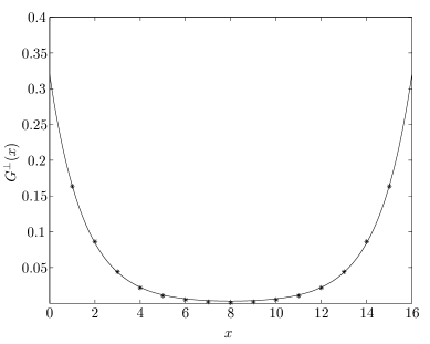
Figure 7: The transverse correlation function along an arbitrary lattice axis, fitted as $G^{\perp}(x)=a_{1}\cosh(M(x-L/2))+a_{2}$ with $a_{1}=0.0048$, $a_{2}=-0.0053$, $M=0.6084$. Data points are obtained with algorithm AI.

The numerical values of the observables, $\mathfrak{M}$, $M$ and the transverse susceptibility,

$$\chi^{\perp}\equiv\sum_{x}G_{x}^{\perp}\;,$$ (11)

which all can be derived from the two–point functions, are summarized in Table 1 for both algorithms.

algorithm	$\mathfrak{M}$	$a^{-4}\chi^{\perp}$	$aM$	$M$ [GeV]
AI	0.438	92.57	0.61	0.95
AII	0.366	79.66	0.67	1.03

Table 1: Numerical results for some observables as obtained from the longitudinal and transverse two–point functions, $G^{\parallel}$ and $G^{\perp}$, respectively.

The disagreement between AI and AII is statistically significant. We attribute it to the ubiquitous Gribov problem [21] (for Abelian gauges, see [22, 23]). On the lattice, this is the statement that maximizing gauge fixing functions like $F_{\mathrm{MAG}}$ or $F_{\mathrm{LLG}}$ is equivalent to a spin–glass problem with an enormous number of degenerate extrema. This implies that the algorithms AI and AII will almost certainly end up in different local maxima, which explains the difference between rows one and two in Table 1.

As shown in the last column of Table 1, the numerical results for the mass gap $M$ lead to a value of about 1 GeV in physical units.

$n^{3}$ is a local functional of the $n^{i}$, $n^{3}=(1-n^{i}n^{i})^{1/2}$. Thus, one expects the same exponential decay for the longitudinal correlator $G^{\parallel}$. This can be confirmed with a numerical value for the mass gap of $M=0.66\;a^{-1}$.

To improve statistics, we have calculated the time–slice correlator,

$$C^{\perp}(t)\equiv L^{-3}\sum_{\mbox{\footnotesize\boldmath$x$}}G^{\perp}_{\mbox{\footnotesize\boldmath$x$},t}\;.$$ (12)

In the continuum, for purely exponential decay of $G^{\perp}$, this would become proportional to a modified Bessel function $K_{2}$. An associated fit works very well as is shown in Fig. 8.

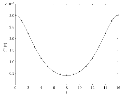
Figure 8: The time–slice correlator fitted to a (properly symmetrized) Bessel function, $C^{\perp}(t)=c_{1}[t^{2}K_{2}(Mt)+(t-L)^{2}K_{2}(M(L-t))]+c_{2}$, where $c_{1}=0.0006$, $c_{2}=0.0001$ and $M=0.6423$. Data points are obtained with algorithm AI.

Fitting the time–slice correlator according to Fig. 8, we obtain for the mass gap

$$aM=0.642\quad\mbox{i.e.}\quad M=0.97\;\mbox{GeV}\;.$$ (13)

This is the value with the smallest statistical errors.

The mass gap obtained differs significantly from the $SU(2)$ mass gap, $M_{SU(2)}\simeq$ 1.5 GeV, obtained directly from a Wilson ensemble with $\beta=2.4$ [24]. We believe that the difference is due to the highly nonlocal relation between the original Yang–Mills degrees of freedom (the link variables) and the color spin $n$. After all, we have implicitly solved the partial differential equation (7) with link variables $U$ in Landau gauge entering the adjoint Laplacian. The solution $n$ will clearly be a nonlocal functional of these $U$’s. Consequently, we cannot expect that the exponential decay of $G^{\perp}[n]$ will be governed by the lowest excitation of the $U$–ensemble.

4 Effective action and Schwinger–Dyson equations

At this point it is natural to ask whether there is an effective action $S_{\mathrm{eff}}[n]$ that reproduces the distribution of $n$–fields leading to the results of the previous section.

At low energies, it should make sense to employ an ansatz in terms of a derivative expansion,

$$S_{\mathrm{eff}}=\sum_{j}\lambda_{j}S_{j}[\mbox{\boldmath$n$}]+\sum_{j}\lambda_{j}^{\prime}\,S_{j}^{\prime}[\mbox{\boldmath$n$},\mbox{\boldmath$h$}]\;,$$ (14)

with $O(3)$ invariant operators $S_{j}$ and noninvariant operators $S_{j}^{\prime}$, which are ordered by increasing mass dimension. Up to dimension four, one has the symmetric terms,

$$\begin{array}[]{lcl}S_{1}=(\mbox{\boldmath$n$},\triangle\mbox{\boldmath$n$})\;,&&S_{2}=(\mbox{\boldmath$n$},\triangle^{2}\mbox{\boldmath$n$})\;,\\ S_{3}=\big{(}\mbox{\boldmath$n$}\cdot\triangle\mbox{\boldmath$n$},\mbox{\boldmath$n$}\cdot\triangle\mbox{\boldmath$n$}\big{)}\;,&&S_{4}=\big{(}\mbox{\boldmath$n$}\cdot\partial_{\mu}^{\dagger}\partial_{\nu}\mbox{\boldmath$n$},\mbox{\boldmath$n$}\cdot\partial_{\mu}^{\dagger}\partial_{\nu}\mbox{\boldmath$n$}\big{)}\;,\end{array}$$ (15)

and the symmetry–breaking terms including a unit vector ‘source field’ $h$ [14] (which can be thought of as the direction of an external magnetic field),

$$S_{1}^{\prime}=(\mbox{\boldmath$n$},\mbox{\boldmath$h$})\;,\quad S_{2}^{\prime}=(\mbox{\boldmath$n$}\cdot\mbox{\boldmath$h$},\mbox{\boldmath$n$}\cdot\mbox{\boldmath$h$})\;,\quad S_{3}^{\prime}=(\mbox{\boldmath$n$}\cdot\triangle\mbox{\boldmath$n$},\mbox{\boldmath$n$}\cdot\mbox{\boldmath$h$})\ .$$ (16)

In the above, we have introduced the scalar products

$$(f,g)\equiv\sum_{x}f_{x}g_{x}\;,\quad\mbox{\boldmath$u$}\cdot\mbox{\boldmath$v$}\equiv u^{a}v^{a}\;,$$ (17)

and the usual lattice Laplacian $\triangle$ (see App. A).

Note that the $n$–field configurations are classified by the Hopf invariant irrespective of the particular form of the (effective) action. This, together with the usual scaling arguments, shows that the action (14) with the operators (15) and (16) should still support classical knot soliton solutions. Our ansatz thus does not exclude this important feature.

The couplings in (14) can be determined by inverse Monte Carlo techniques. The notion is suggestive: instead of creating an ensemble from a given action, one wants to compute a (truncated) action which gives rise to the given ensemble of $n$–fields. A particular approach uses the Schwinger–Dyson equations [25, 26]. These represent an overdetermined linear system which can be used to solve for the couplings in terms of correlation functions. The latter are nothing but the coefficients of the linear system.

For an unconstrained scalar field $\phi$, the Schwinger–Dyson equations follow from translational invariance of the functional measure, implying

$$0=\int\mathcal{D}\phi\,\mathbb{P}_{x}\Big{\{}F[\phi]\exp(-S[\phi])\Big{\}}\;,$$ (18)

where $\mathbb{P}_{x}\equiv-i\delta/\delta\phi_{x}$ is the (functional) momentum operator, and $F$ an arbitrary functional of the field $\phi$. For a constrained field like $n$ with a curved target space things are slightly more subtle [25]. There is, however, a rather elegant way to derive the Schwinger–Dyson equations if one exploits the isometries of the target space $S^{2}$ [27]. The target space measure,

$$\mathcal{D}\mbox{\boldmath$n$}=\prod_{x}d\mbox{\boldmath$n$}_{x}\,\delta\big{(}\mbox{\boldmath$n$}_{x}^{2}-1\big{)}\;,$$ (19)

is obviously rotationally invariant, i.e. under $\mbox{\boldmath$n$}\to R\mbox{\boldmath$n$}$, $R\in O(3)$. This implies the modified Schwinger–Dyson identity

$$\int\mathcal{D}\mbox{\boldmath$n$}\,\mbox{\boldmath$L$}_{x}\,\Big{\{}F[\mbox{\boldmath$n$}]\exp\big{(}-S_{\mathrm{eff}}[\mbox{\boldmath$n$},\mbox{\boldmath$h$}]\big{)}\Big{\}}=0\;,$$ (20)

where $\mbox{\boldmath$L$}_{x}$ denotes the angular momentum operator (at lattice site $x$),

$$i\mbox{\boldmath$L$}_{x}=\mbox{\boldmath$n$}_{x}\times\frac{\partial}{\partial\mbox{\boldmath$n$}_{x}}\quad\hbox{or}\quad iL_{x}^{a}\equiv\epsilon^{abc}n_{x}^{b}\frac{\delta}{\delta n_{x}^{c}}\;.$$ (21)

In shorthand–notation, (20) can be rewritten as

$$\langle\mbox{\boldmath$L$}_{x}\,F[\mbox{\boldmath$n$}]-F[\mbox{\boldmath$n$}]\mbox{\boldmath$L$}_{x}\,S_{\mathrm{eff}}[\mbox{\boldmath$n$}]\rangle=0\;.$$ (22)

These exact identities can be used to determine the unknown couplings $\lambda_{j}$. To this end one chooses a set of field monomials $F_{i}[\mbox{\boldmath$n$}]$ and plugs them into (22) together with the form (14) of the action. This yields the local linear system

$$\sum_{j}\langle F_{i}\,\mbox{\boldmath$L$}_{x}\,S_{j}\rangle\lambda_{j}+\sum_{k}\langle F_{i}\,\mbox{\boldmath$L$}_{x}\,S_{k}^{\prime}\rangle\lambda_{k}^{\prime}=\langle\mbox{\boldmath$L$}_{x}\,F_{i}\rangle\;,$$ (23)

which, in principle, can be solved numerically, for instance by least–square methods. The identities obtained so far hold for arbitrary actions $S_{\mathrm{eff}}[\mbox{\boldmath$n$}]$. In particular, we have not made use of any symmetries. Taking the latter into account will lead to Ward identities.

Let us specialize to our lattice effective action (14). It is a sum of a symmetric part $S$ containing the terms (15) and an asymmetric part $S^{\prime}$ containing the terms (16),

$$S_{\mathrm{eff}}=S[\mbox{\boldmath$n$}]+S^{\prime}[\mbox{\boldmath$n$},\mbox{\boldmath$h$}]\;.$$ (24)

Due to the invariance of $S$ under global $O(3)$ rotations it is an $O(3)$–singlet and hence annihilated by the total angular momentum,

$$\mbox{\boldmath$L$}S=0,\qquad\mbox{\boldmath$L$}=\sum_{x}\mbox{\boldmath$L$}_{x}\;,$$ (25)

such that $\mbox{\boldmath$L$}S_{\mathrm{eff}}=\mbox{\boldmath$L$}S^{\prime}$. Thus, summing over all lattice sites $x$ in (22) yields the (broken) Ward identity,

$$\langle\mbox{\boldmath$L$}F[\mbox{\boldmath$n$}]-F[\mbox{\boldmath$n$}]\,\mbox{\boldmath$L$}S^{\prime}[\mbox{\boldmath$n$},\mbox{\boldmath$h$}]\rangle=0\;,$$ (26)

where the second terms contains the infinitesimal change of the non-invariant part $S^{\prime}$ of the effective action under rotations of $n$. Note that the coupling constants $\lambda_{j}$ of the $O(3)$–symmetric operators $S_{j}$ have disappeared in the Ward identity (26) so that only the symmetry–breaking couplings $\lambda^{\prime}$ are present. We have collected the explicit lattice Schwinger–Dyson and Ward identities used in our simulations in App. C. As the former are local relations, they naturally contain more information than the global Ward identities. In particular, one does have access to length scales.

5 Comparing Yang–Mills and FN ensembles

5.1 Leading–order ansatz

To leading order (LO) in the derivative expansion we have a standard nonlinear sigma model with symmetry–breaking term,

$$S_{\mathrm{eff}}=\sum_{x}(\lambda\mbox{\boldmath$n$}_{x}\cdot\triangle\mbox{\boldmath$n$}_{x}+\lambda^{\prime}\mbox{\boldmath$n$}_{x}\cdot\mbox{\boldmath$h$})\;,\quad\mbox{\boldmath$h$}\equiv\mbox{\boldmath$e$}_{z}\;.$$ (27)

Inverse Monte Carlo amounts to determining the couplings $\lambda$ and $\lambda^{\prime}$ such that the probability distribution associated with the LO action (27) fits the observables of the Yang–Mills ensemble of $n$–fields. The associated Schwinger–Dyson equation (23), with $F[\mbox{\boldmath$n$}]=n_{x}^{a}$, can be written as

$$\lambda H_{xy}+\lambda^{\prime}G^{\perp}_{xy}=-\mathfrak{M}\,\delta_{xy}\;,$$ (28)

where $H$ denotes the (antisymmetrized) two–point function of $n^{i}$ and $n^{i}\triangle n^{3}$,

$$H_{xy}\equiv\langle n_{x}^{i}n_{y}^{i}\triangle n_{y}^{3}\rangle-\langle n_{x}^{i}n_{y}^{3}\triangle n_{y}^{i}\rangle\equiv\langle n_{x}^{i}n_{y}^{[\,i}\triangle n_{y}^{3]}\rangle\;.$$ (29)

To analyse (28) we define a ‘reduced’ two–point function $h_{xy}$ and magnetization $\mu$,

$$h_{xy}\equiv H_{xy}/G_{xy}^{\perp}\;,\quad\mu\equiv\mathfrak{M}/G_{xx}^{\perp}\;,$$ (30)

and rewrite (28) as the inhomogeneous system (using translational invariance to replace $x-y\to x$),

$$\lambda h_{x}+\lambda^{\prime} = 0\;,\quad x=1,\ldots,8\;,$$ (31)

$$\lambda h_{0}+\lambda^{\prime} = -\mu\;.$$ (32)

The solution is found to be

$$\lambda = \phantom{-}\frac{1}{h_{x}-h_{0}}\,\mu\;,$$ (33)

$$\lambda^{\prime} = -\frac{h_{x}}{h_{x}-h_{0}}\,\mu\;,$$ (34)

with the numerical boundary value given by $h_{0}=0.1410$ (cf. Fig. 9). Clearly, the system (31), (32) is overdetermined (nine equations for two unknowns). This is reflected in the fact that $\lambda$ and $\lambda^{\prime}$ in (33) and (34) depend on the lattice distance $x$ via $h_{x}$. If the Yang–Mills ensemble were exactly described by the LO action (27), there would be no such $x$–dependence. Rather, for any $x=1,\ldots,8$, we would have the same values for $\lambda$ and $\lambda^{\prime}$, respectively. Thus, to test the quality of the LO ansatz, we divide (34) by (33) showing explicitly that $h_{x}$ should be constant,

$$h_{x}=-\frac{\lambda^{\prime}}{\lambda}\equiv-\kappa^{\prime}=const.\;,\quad x\neq 0\;.$$ (35)

Fig. 9 shows that this is not the case.

Figure 9: $h_{x}$ for the Yang–Mills ensemble. The boundary value is $h_{0}=0.1410$.

Therefore, a minimal sigma model with symmetry–breaking term does not yield a good representation of our Yang–Mills ensemble of $n$–fields. If we nevertheless insist on the LO description, we have to ‘fit’ $h_{x}$ by a horizontal line so that the numerical determination of the couplings via (33) and (34) is beset by large errors,

$$\lambda = -1.41\pm 5.25\;,$$ (36)

$$\lambda^{\prime} = -1.33\pm 0.74\;.$$ (37)

Obviously, $\lambda$ (including its sign) remains essentially undetermined. For $\lambda^{\prime}$ the situation is slightly better.

In order to assess the errors it is worthwhile to check whether our numerical accuracy is sufficient to really validate the Schwinger–Dyson identity (28) for the LO action (27) on the lattice. To this end we have simulated (27) with a combination of Metropolis and cluster algorithms producing a number of 150 configurations using the central values (36) and (37) as the input couplings. The result for $h_{x}$ in the LO ensemble is presented in Fig. 10.

Figure 10: $h_{x}$ for the LO ensemble. Fitting the data points yields $h_{x}=-\kappa^{\prime}=-0.938\pm 0.002$.

It is reassuring to note that the simulation of the minimal sigma model reproduces the input value $\kappa^{\prime}=0.943$ very well (for $x\neq 0$), the error being of the order of one percent. The prediction (35) thus can be verified with high accuracy for the LO action (27). We conclude that inverse Monte Carlo works quite well when applied to the minimal $\sigma$–model.

The discrepancy between the LO and Yang–Mills ensembles can be further visualized by looking at the susceptibility. For the action (27) and the choice $F[\mbox{\boldmath$n$}]=n_{x}^{a}$, the Ward identity (26) assumes the simple form

$$\chi^{\perp}=-\mathfrak{M}/\lambda^{\prime}\;.$$ (38)

A consistency check is provided by noting that this can directly be obtained by summing (28) over $x$. Plugging in the magnetization from Table 1 and $\lambda^{\prime}$ from (37) we find

$$\chi^{\perp}=0.33\pm 0.18\;,$$ (39)

This is way off the Yang–Mills value of 92.6 displayed in Table 1. For magnetization and mass gap the simulation of the LO ensemble yields the values

$$\mathfrak{M}=0.93\;,\quad M=1.5\;,$$ (40)

which are both larger than the Yang–Mills values of Table 1.

The discussion of this subsection thus shows quite clearly that more operators will have to be included in order to possibly make inverse Monte Carlo work reasonably well.

5.2 FN action with symmetry–breaking term

In this subsection we consider the FN action (1) with a LO symmetry–breaking term,

$$S_{\mathrm{eff}}=\sum_{x}\left\{\lambda\mbox{\boldmath$n$}_{x}\cdot\triangle\mbox{\boldmath$n$}_{x}+\lambda_{\mbox{\tiny FN}}\left[(\mbox{\boldmath$n$}\cdot\triangle\mbox{\boldmath$n$})^{2}-(\mbox{\boldmath$n$}\cdot\partial_{\mu}^{\dagger}\partial_{\nu}\mbox{\boldmath$n$})^{2}\right]+\lambda^{\prime}\mbox{\boldmath$n$}_{x}\cdot\mbox{\boldmath$h$}\right\}\;.$$ (41)

This ansatz does not include all terms of next–to–leading order (NLO) in the derivative expansion. It should be viewed as a minimal modification of the original FN action by adding an explicit symmetry–breaking term to obtain a mass gap.

The Schwinger–Dyson equation generalizing (28) becomes

$$\lambda H_{xy}+\lambda_{\mbox{\tiny FN}}H_{xy}^{\mbox{\tiny FN}}+\lambda^{\prime}G_{xy}^{\perp}=-\mathfrak{M}\,\delta_{xy}\;.$$ (42)

The new two–point function $H^{\mbox{\tiny FN}}$ is given by (90). The local identities (42) are to be solved for the three unknown couplings $\lambda$, $\lambda^{\prime}$ and $\lambda_{\mbox{\tiny FN}}$.

Figure 11: $h^{\mbox{\tiny FN}}_{x}$ for the Yang–Mills ensemble. The boundary value $h_{0}^{\mbox{\tiny FN}}=-31.24$ is not displayed.

Introducing another reduced two–point function,

$$h_{xy}^{\mbox{\tiny FN}}\equiv H_{xy}^{\mbox{\tiny FN}}/G_{xy}^{\perp}\;,$$ (43)

which is plotted in Fig. 11, we obtain, instead of (31) and (32), the (overdetermined) system,

$$\lambda h_{x}+\lambda_{\mbox{\tiny FN}}h_{x}^{\mbox{\tiny FN}}+\lambda^{\prime} = 0\;,\quad x=1,\ldots,8\;;$$ (44)

$$\lambda h_{y}+\lambda_{\mbox{\tiny FN}}h_{y}^{\mbox{\tiny FN}}+\lambda^{\prime} = 0\;,\quad y>x\;;$$ (45)

$$\lambda h_{0}+\lambda_{\mbox{\tiny FN}}h_{0}^{\mbox{\tiny FN}}+\lambda^{\prime} = -\mu\;,$$ (46)

to be solved for each pair of lattice distances $(x,y)$, $y>x$. The number of independent pairs is $7(7+1)/2=28$ for lattice extension $L=16$. The solutions, labelled by $x$ and $y$, are

$$\lambda = \frac{h_{x}^{\mbox{\tiny FN}}-h_{y}^{\mbox{\tiny FN}}}{d_{xy}}\,\mu\;,$$ (47)

$$\lambda^{\prime} = \frac{h_{x}h_{y}^{\mbox{\tiny FN}}-h_{y}h_{x}^{\mbox{\tiny FN}}}{d_{xy}}\,\mu\;,$$ (48)

$$\lambda_{\mbox{\tiny FN}} = -\frac{h_{x}-h_{y}}{d_{xy}}\,\mu\;,$$ (49)

where we have defined the determinant

$$d_{xy}\equiv h_{0}(h_{x}^{\mbox{\tiny FN}}-h_{y}^{\mbox{\tiny FN}})-h_{0}^{\mbox{\tiny FN}}(h_{x}-h_{y})+h_{x}h_{y}^{\mbox{\tiny FN}}-h_{y}h_{x}^{\mbox{\tiny FN}}\;.$$ (50)

We have checked that the numerical values for $d_{xy}$ are not close to zero so that there is no problem with small denominators in the solutions.

Figure 12: Variation of the couplings (47–49) with lattice distances $x$ and $y$. The values associated with $y>x$ are plotted along vertical lines labelled by $x=1,\ldots,8$. The horizontal lines denote the mean value. Note that, for larger distances, the data seem to deviate less from the central values. (a) coupling $\lambda$, (b) coupling $\lambda^{\prime}$, (c) coupling $\lambda^{\mbox{\tiny FN}}$.

For each pair of lattice distances $(x,y)$ we thus have a certain value for any of the three couplings (47–49). For each particular coupling those would all agree (within statistical errors) if the NLO action (41) would exactly describe the Yang–Mills ensemble. Again, however, analogous to the LO case, the couplings do vary with lattice distances $x$ and $y$ as shown in Fig. 12. Numerically, one finds,

$$\lambda = -0.232\pm 0.035\;,$$ (51)

$$\lambda^{\prime} = \phantom{-}0.257\pm 0.014\;,$$ (52)

$$\lambda_{\mbox{\tiny FN}} = -0.0402\pm 0.0004\;.$$ (53)

Several remarks are in order. First of all, the relative errors, given by the standard deviation from the mean (see Fig. 12), are small compared to the LO ansatz. In particular, the signs of all couplings are fixed. Interestingly, the addition of the FN coupling $\lambda_{\mbox{\tiny FN}}$, although small numerically, has a large effect: it reverts the sign of $\lambda^{\prime}$ as compared to (37), implying a negative magnetization. This follows, for instance, from the Ward identity (38), which still holds for the action (41), and the positivity of the susceptibility, hence

$$\mathfrak{M}=-\lambda^{\prime}\chi^{\perp}<0\;,$$ (54)

in contradistinction with the positive Yang–Mills value of Table 1.

To further analyse the result for the couplings, we divide (44) by $\lambda$, leading to a linear relation between $h$ and $h^{\mbox{\tiny FN}}$ (for $x\neq 0$),

$$h_{x}=-\kappa^{\prime}-\kappa_{\mbox{\tiny FN}}h_{x}^{\mbox{\tiny FN}}\;,\quad\kappa_{\mbox{\tiny FN}}\equiv\lambda_{\mbox{\tiny FN}}/\lambda\;.$$ (55)

Thus, plotting $h_{x}$ against $h_{x}^{\mbox{\tiny FN}}$ should yield a straight line with intercept $-\kappa^{\prime}$ and slope $-\kappa_{\mbox{\tiny FN}}$. The numerical values (51–53) yield

$$\kappa^{\prime}=-1.108\pm 0.228\;,\quad\kappa_{\mbox{\tiny FN}}=0.173\pm 0.024\;.$$ (56)

In analogy with the LO case, we have numerically checked the prediction (55) for the NLO action (41) by a Monte Carlo simulation with 150 configurations using the input couplings (51–53). Fig. 13 clearly demonstrates the expected linear behavior. A corresponding fit results in

$$\kappa^{\prime}=-1.120\;,\quad\kappa_{\mbox{\tiny FN}}=0.171\;,$$ (57)

being consistent with the central values of (56) to within one percent.

Figure 13: $h$ vs. $h^{\mbox{\tiny FN}}$ for the NLO action (41).

We thus conclude that inverse Monte Carlo also works quite well for the NLO ensemble. For the sake of explicit comparison with Fig.s 9 and 11 we display the reduced two–point functions obtained by simulating the NLO action in Fig.s 14 and 15.

Figure 14: $h_{x}$ for the NLO ensemble.

Figure 15: $h^{\mbox{\tiny FN}}_{x}$ for the NLO ensemble.

As expected, the NLO simulation yields a negative magnetization,

$$\mathfrak{M}=-0.49\;,$$ (58)

while the mass gap becomes $M=1.2$, i.e. slightly larger than the value listed in Table 1.

If the Yang–Mills ensemble has anything to do with the FN one, then plotting $h$ vs. $h^{\mbox{\tiny FN}}$ (as obtained from Yang–Mills) should also show straight–line behavior, at least approximately. Fig. 16 displays a linear fit to the the Yang–Mills data with parameters

$$\kappa^{\prime}=-1.232\;,\quad\kappa_{\mbox{\tiny FN}}=0.170\;.$$ (59)

Figure 16: $h$ vs. $h^{\mbox{\tiny FN}}$ for the Yang–Mills ensemble. The error bars reflect the fact that, for large distances $x$ (i.e. $x\simeq L/2=8$ for the lattice size used), $h$ and $h^{\mbox{\tiny FN}}$ are obtained by dividing two small numbers (from the tails of the two–point functions $G^{\perp}$, $H$ and $H^{\mbox{\tiny FN}}$).

Again, within error bars, these values are consistent with the preceding analysis (56). Note that reverting the sign of $\lambda^{\prime}$ amounts to reverting the sign of the intercept in Fig. 16. The data points clearly do not support anything like that. On the contrary, it seems that, for small $h^{\mbox{\tiny FN}}$ (corresponding to small distances $x$, see Fig. 11), the data points deviate from a straight line. Playing around with different fits indicates that $h$ rises with a negative power of $h^{\mbox{\tiny FN}}$ for small $h^{\mbox{\tiny FN}}$ so that in reality there may be no intercept at all.

The behavior of $\kappa^{\prime}$ as a function of lattice distances $x$ and $y$ may also be investigated. Dividing (48) by (47) we find

$$\kappa^{\prime}=\lambda^{\prime}/\lambda=\frac{h_{x}h_{y}^{\mbox{\tiny FN}}-h_{y}h_{x}^{\mbox{\tiny FN}}}{h_{x}^{\mbox{\tiny FN}}-h_{y}^{\mbox{\tiny FN}}}=-1.38\pm 0.29\;,$$ (60)

where, in the analytic expression, the determinant $d_{xy}$ has dropped out. Fig. 17 shows the variation of $\kappa^{\prime}$ with $x$ and $y$. Again, a different sign for $\kappa^{\prime}$ is completely out of reach.

Figure 17: Variation of $\kappa^{\prime}$ with lattice distances $x$ and $y$. The central value is $\kappa^{\prime}=-1.38$.

Following the logic of gradient expansions, one may argue that the effective action (41) is supposed to represent the Yang–Mills ensemble only for large distances. Fig. 16, for instance, seems to indicate that the straight–line fit works particularly well for the last three points to the right which correspond to $x=6,7,8$, respectively. In physical units, this amounts to distances $R$ larger than six lattice units, i.e. $R$ $\scriptstyle{\stackrel{{\scriptstyle>}}{{\sim}}}$ 0.8 fm. Restricting to the analogous data points in Fig. 12, we obtain for the couplings in (41),

$$\lambda = -0.2775\pm 0.026\;,$$ (61)

$$\lambda^{\prime} = \phantom{-}0.2661\pm 0.012\;,$$ (62)

$$\lambda^{\mbox{\tiny FN}} = -0.040\pm 0.0005\;,$$ (63)

and for the ‘reduced’ ones,

$$\kappa^{\prime}=-0.97\pm 0.13\;,\quad\kappa^{\mbox{\tiny FN}}=0.15\pm 0.01\;.$$ (64)

All these do not differ significantly from the values (51–53) and (56) obtained by using the unrestricted data set. In particular, the sign of $\lambda^{\prime}$ remains positive. We therefore conclude that, also at large distances, the minimally modified FN action (41) fails to describe the Yang–Mills ensemble of $n$–fields.

6 Summary and discussion

We have performed a lattice test of the FN conjecture stating that low–energy $SU(2)$ Yang–Mills theory is equivalent to a Skyrme–type sigma model. More specifically, FN suggest that the knot solitons of their model might be related to the Yang–Mills glueball spectrum.

Using standard Monte Carlo techniques, we have generated an ensemble of $SU(2)$ link fields from the Wilson action. This ensemble was then used to extract an associated ensemble of color vectors $n$, with $n$ parametrizing the gauge invariant distance between the maximally–Abelian and lattice Landau gauge slices. As these gauges are close to each other, there is a preferred direction for the $n$–field which corresponds to explicit symmetry breaking. In this way we avoid the appearance of massless Goldstone bosons and thus generate a nonvanishing mass gap. A study of the exponential decay of correlators yields a mass gap close to 1 GeV. To find the effective action describing the Yang–Mills ensemble of $n$–fields we have employed inverse Monte Carlo techniques. These are based on Schwinger–Dyson and Ward identities which we have derived analytically on the lattice. The identities have been evaluated numerically for the Yang–Mills ensemble on the one hand, and for ensembles stemming from LO and NLO effective actions on the other hand. As a result, we have found strong evidence that the ensemble generated from Yang–Mills theory cannot be described by the FN action plus a minimal symmetry–breaking term to allow for a mass gap. This follows from a number of discrepancies between the two ensembles. First, and most prominent, the sign of $\lambda^{\prime}$ is positive, implying negative magnetization $\mathfrak{M}$, at variance with the value from the Yang–Mills ensemble. Second, the reduced two–point function $h$ ($h^{\mbox{\tiny FN}}$) from the NLO ensemble increases (decreases) with lattice disctance $x$, while for Yang–Mills the behavior is just the opposite. Third, the size of the mass gap is larger than for the Yang–Mills ensemble of $n$–fields.

It is quite conceivable that magnetization (and susceptibility) can be recovered correctly by adding more (symmetry–breaking) terms to the NLO action (work in this direction is under way). The same remark applies to the mass gap. Note, however, that one cannot naturally expect the Yang–Mills and $\sigma$–model mass gaps to coincide due to the nonlocal relation between $n$ and the link variables $U$. Whether this represents a problem is a question of scales. If the effective $\sigma$–model were valid only for distances of, say, $R$ $\scriptstyle{\stackrel{{\scriptstyle>}}{{\sim}}}$ 0.8 fm corresponding to energies $E$ $\scriptstyle{\stackrel{{\scriptstyle<}}{{\sim}}}$ 0.25 GeV, as suggested by the discussion of Section 5, then it would make no sense to address questions like the glueball spectrum. An analogous situation holds for the Fermi theory of weak interactions which also is only effective much below the $W$ and $Z$ scales.

Finally, one should mention that there is still another fundamental problem associated with describing Yang–Mills theory in terms of effective $\sigma$–models. Allowing for finite temperature, the latter are in the universality class of the 4$d$ Heisenberg model, while $SU(2)$ Yang–Mills theory is in the 3$d$ Ising class [28]. This issue has been discussed recently in the context of constructing effective actions via Abelian projections [29, 30, 31]. Again, if the $\sigma$–model scale were below the critical temperature, the effective theory would only be valid in the confined phase and would have nothing to say about the behavior of Yang–Mills theory close to the phase transition. Otherwise, an infinite number of operators would be required which, of course, is anything else but an ‘effective’ description. Summarizing, we conclude that, while a reasonable effective model generalizing the FN action may exist in principle, it will be of little practical use.

Appendix A Conventions

Left and right lattice derivatives are defined as

$$\partial_{\mu}f_{x} \equiv f_{x+\mu}-f_{x}\;,$$ (65)

$$\partial_{\mu}^{\dagger}f_{x} \equiv f_{x-\mu}-f_{x}\;.$$ (66)

The ordinary lattice Laplacian $\triangle\equiv-\partial_{\mu}^{\dagger}\partial_{\mu}$ is a negative semi–definite operator. Its action on lattice functions $f$ is given by

$$\triangle f_{x}\equiv-\sum_{\mu}(2f_{x}-f_{x+\mu}-f_{x-\mu})\;.$$ (67)

The covariant Laplacian $\triangle[U]$ in the adjoint representation acts as

$$\triangle^{ab}[U]f_{x}^{b}\equiv-\sum_{\mu}\left(2f_{x}^{a}-R_{x,\mu}^{ab}\,f_{x+\mu}^{b}-R_{x-\mu,\mu}^{ba}\,f_{x-\mu}^{b}\right)\;,$$ (68)

where we have defined the adjoint link

$$R_{x,\mu}^{ab}\equiv\frac{1}{2}\mbox{tr}(\tau^{a}U_{x,\mu}\tau^{b}U_{x,\mu}^{\dagger})\;.$$ (69)

Appendix B Relating LLG and MAG

From (9) it follows immediately that the LLG minimizes the functional [32]

$$\bar{F}_{\mathrm{LLG}}\equiv\sum_{l}\mbox{tr}(\Eins-{}^{\Omega}U_{l})\;,\quad l\equiv(x,\mu)\;,$$ (70)

and thus tends to bring the links $U_{l}$ close to $\Eins$. The MAG, on the other hand, minimizes

$$\bar{F}_{\mathrm{MAG}}\equiv\sum_{l}(1-{}^{g}R_{l}^{33})\;,$$ (71)

and thus wants to bring the 33–entry of the adjoint link $R_{l}^{ab}$ close to 1. From (69) it is obvious that, if $U_{l}$ equals unity, the same will be true for $R_{l}$. This can be made more precise: if $U_{l}\simeq\Eins+iaA_{l}$, $A_{l}$ hermitean, then it is an easy exercise to show that $R_{l}^{33}=1+O(a^{2})$. In this sense, the LLG is close to the MAG.

Appendix C Schwinger–Dyson equations and Ward identities

We begin with computing the infinitesimal rotations of the various contributions in (15) and (16) to the effective action. It turns out that, for all $S_{j}$, the action of the angular momentum can be written as

$$i\mbox{\boldmath$L$}_{x}S_{j}=\mbox{\boldmath$n$}_{x}\times\mbox{\boldmath$K$}_{jx}\;,$$ (72)

(and analogous for the $S_{k}^{\prime}$) with the vectors $\mbox{\boldmath$K$}_{jx}$ and $\mbox{\boldmath$K$}_{kx}^{\prime}$ given by

$$\mbox{\boldmath$K$}_{1x} = 2\triangle\mbox{\boldmath$n$}_{x}$$ (73)

$$\mbox{\boldmath$K$}_{2x} = 2\triangle^{2}\,\mbox{\boldmath$n$}_{x}$$ (74)

$$\mbox{\boldmath$K$}_{3x} = 2\left[\triangle\mbox{\boldmath$n$}_{x}(\mbox{\boldmath$n$}_{x}\cdot\triangle\mbox{\boldmath$n$}_{x})+\triangle\left(\mbox{\boldmath$n$}_{x}(\mbox{\boldmath$n$}_{x}\cdot\triangle\mbox{\boldmath$n$}_{x})\right)\right]$$ (75)

$$\mbox{\boldmath$K$}_{4x} = 2\left[\partial_{\mu}^{\dagger}\partial_{\nu}\mbox{\boldmath$n$}_{x}(\mbox{\boldmath$n$}_{x}\cdot\partial_{\mu}^{\dagger}\partial_{\nu}\mbox{\boldmath$n$}_{x})+\partial_{\mu}^{\dagger}\partial_{\nu}\left(\mbox{\boldmath$n$}_{x}(\mbox{\boldmath$n$}_{x}\cdot\partial_{\mu}^{\dagger}\partial_{\nu}\mbox{\boldmath$n$}_{x})\right)\right]$$ (76)

$$\mbox{\boldmath$K$}_{1x}^{\prime} = h$$ (77)

$$\mbox{\boldmath$K$}_{2x}^{\prime} = 2\mbox{\boldmath$h$}\,(\mbox{\boldmath$n$}_{x}\cdot\mbox{\boldmath$h$})$$ (78)

$$\mbox{\boldmath$K$}_{3x}^{\prime} = \mbox{\boldmath$h$}\,(\mbox{\boldmath$n$}_{x}\cdot\triangle\mbox{\boldmath$n$}_{x})+\triangle\mbox{\boldmath$n$}_{x}(\mbox{\boldmath$n$}_{x}\cdot\mbox{\boldmath$h$})+\triangle(\mbox{\boldmath$n$}_{x}(\mbox{\boldmath$n$}_{x}\cdot\mbox{\boldmath$h$}))\;.$$ (79)

Choosing the $F$’s in (26) as $n_{x}^{a}$, $n_{x}^{a}n_{y}^{b}$ and $n_{x}^{a}n_{y}^{b}n_{z}^{c}$, respectively, results in the Ward identities

$$G_{\underline{x}y}^{ii}\lambda_{1}^{\prime}+2G_{\underline{x}\underline{x}y}^{3ii}\lambda_{2}^{\prime}+G_{\underline{x}\underline{x}y}^{\Delta ii}\lambda_{3}^{\prime} = -2G_{y}^{3}\;,$$ (80)

$$G_{\underline{x}yz}^{ii3}\lambda_{1}^{\prime}+2G_{\underline{x}\underline{x}yz}^{3ii3}\lambda_{2}^{\prime}+G_{\underline{x}\underline{x}yz}^{\Delta ii3}\lambda_{3}^{\prime} = -2G_{yz}^{33}+G_{yz}^{ii}\;,$$ (81)

$$G_{\underline{x}yzz^{\prime}}^{ii33}\lambda_{1}^{\prime}+2G_{\underline{x}\underline{x}yzz^{\prime}}^{3ii33}\lambda_{2}^{\prime}+G_{\underline{x}\underline{x}yzz^{\prime}}^{\Delta ii33}\lambda_{3}^{\prime} = -2G_{yzz^{\prime}}^{333}+2G_{yzz^{\prime}}^{i(i3)}\;.$$ (82)

Here, the superscript $(i3)$ denotes symmetrization in $i$, 3, and we have introduced the shorthand notations

$$G_{xyz\ldots}^{abc\ldots} \equiv \langle n_{x}^{a}n_{y}^{b}n_{z}^{c}\ldots\rangle\;,$$ (83)

$$G_{\underline{x}y\ldots}^{ii\ldots} \equiv \sum_{x}G_{xy\ldots}^{ii\ldots}\;,$$ (84)

$$G_{\underline{x}\underline{x}y\ldots}^{3ii\ldots} \equiv \sum_{x}\langle n_{x}^{3}n_{x}^{i}n_{y}^{i}\ldots\rangle\;,$$ (85)

$$G_{\underline{x}\underline{x}y\ldots}^{\Delta ii\ldots} \equiv \sum_{x}\langle(n_{x}^{a}\triangle n_{x}^{a})n_{x}^{i}n_{y}^{i}\ldots\rangle\;,$$ (86)

with $\underline{x}$ denoting summation over all lattice sites $x$. In particular, one has

$$G_{y}^{3}\equiv\mathfrak{M}\;,\quad G_{\underline{x}y}^{ii}\equiv 2\chi^{\perp}\;,\quad G_{xy}^{ii}\equiv 2G_{xy}^{\perp}\;,\quad\quad G_{xy}^{33}\equiv G_{xy}^{\parallel}\;.$$ (87)

It seems that a particular recurrence pattern arises in (80–82) that could be used to derive a Ward identity for an insertion of an arbitrary number of $n$’s. For the NLO derivative expansion, however, the three identities are sufficient to determine the symmetry–breaking couplings $\lambda^{\prime}$.

For the particular case that $F$ in (23) equals $n$, $F_{x}^{a}=n_{x}^{a}$, we can give the general Schwinger–Dyson equation in closed form,

$$\sum_{j}\lambda_{j}H_{j,xy}+\sum_{k}\lambda_{k}^{\prime}H_{k,xy}^{\prime}=-\mathfrak{M}\delta_{xy}\;,$$ (88)

where we have introduced the two–point function

$$H_{j,xy}\equiv\langle n_{x}^{i}n_{y}^{[\,i}K_{jy}^{3]}\rangle\;,$$ (89)

and, completely analogous, $H_{k,xy}^{\prime}$. The FN terms are (75) minus (76), so that the relevant two–point function becomes

$$H_{xy}^{\mbox{\tiny FN}}\equiv H_{3,xy}-H_{4,xy}\;,$$ (90)

which has been used in (42).

References

- [1] L. Faddeev and A. Niemi, Partially dual variables in SU(2) Yang-Mills theory, Phys. Rev. Lett. 82 (1999) 1624, [hep-th/9807069].
- [2] L. Faddeev and A. Niemi, Knots and particles, Nature 387 (1997) 58, [hep-th/9610193].
- [3] R. Battye and P. Sutcliffe, Knots as stable soliton solutions in a three-dimensional classical field theory, Phys. Rev. Lett. 81 (1998) 4798, [hep-th/9808129].
- [4] J. Hietarinta and P. Salo, Faddeev-Hopf knots: Dynamics of linked unknots, Phys. Lett. B451 (1999) 60, [hep-th/9811053].
- [5] P. van Baal and A. Wipf, Classical gauge vacua as knots, Phys. Lett. B515 (2001) 181, [hep-th/0105141].
- [6] E. Langmann and A. Niemi, Towards a string representation of infrared SU(2) Yang-Mills theory, Phys. Lett. B463 (1999) 252, [hep-th/9905147].
- [7] S. Shabanov, An effective action for monopoles and knot solitons in Yang-Mills theory, Phys. Lett. B458 (1999) 322, [hep-th/9903223].
- [8] S. Shabanov, Yang-Mills theory as an Abelian theory without gauge fixing, Phys. Lett. B463 (1999) 263, [hep-th/9907182].
- [9] H. Gies, Wilsonian effective action for SU(2) Yang-Mills theory with Cho-Faddeev-Niemi-Shabanov decomposition, Phys. Rev. D63 (2001) 125023, [hep-th/0102026].
- [10] F. Freire, Abelian projected SU(2) Yang-Mills action for renormalisation group flows, Phys. Lett. B526 (2002) 405, [hep-th/0110241].
- [11] S. Shabanov, Infrared Yang-Mills theory as a spin system: A lattice approach, Phys. Lett. B522 (2001) 201, [hep-lat/0110065].
- [12] N. Manton, The force between ‘t Hooft-Polyakov monopoles, Nucl. Phys. B126 (1977) 525.
- [13] Y. Cho, Restricted gauge theory, Phys. Rev. D21 (1980) 1080.
- [14] L. Dittmann, T. Heinzl, and A. Wipf, A lattice study of the Faddeev-Niemi effective action, Nucl. Phys. Proc. Suppl. 106 (2002) 649, [hep-lat/0110026].
- [15] L. D. Faddeev and A. J. Niemi, Electric-magnetic duality in infrared SU(2) Yang-Mills theory, Phys. Lett. B525 (2002) 195, [hep-th/0101078].
- [16] G. ‘t Hooft, Gauge theories with unified weak, electromagnetic and strong interactions, in: High Energy Physics, Proceedings of the EPS International Conference, Palermo 1975, A. Zichichi, ed., Editrice Compositori, Bologna 1976.
- [17] A. S. Kronfeld, M. L. Laursen, G. Schierholz, and U.-J. Wiese, Monopole condensation and color confinement, Phys. Lett B198 (1987) 516.
- [18] R. C. Brower, K. N. Orginos, and C.-I. Tan, Magnetic monopole loop for Yang-Mills instanton, Phys. Rev. D55 (1997) 6313, [hep-th/9610101].
- [19] T. Kovacs and E. Tomboulis, On P-vortices and the Gribov problem, Phys. Lett. B463 (1999) 104, [hep-lat/9905029].
- [20] C. Davies, G. Batrouni, G. Katz, A. Kronfeld, G. Lepage, K. Wilson, , P. Rossi, and B. Svetitsky, Fourier acceleration in lattice gauge theories. 1. Landau gauge fixing, Phys. Rev. D37 (1988) 1581.
- [21] V. Gribov, Quantization of non-Abelian gauge theories, Nucl. Phys. B139 (1978) 1.
- [22] F. Bruckmann, T. Heinzl, T. Tok, and A. Wipf, Instantons and Gribov copies in the maximally Abelian gauge, Nucl. Phys. B584 (2000) 589, [hep-th/0001175].
- [23] F. Bruckmann, T. Heinzl, T. Vekua, and A. Wipf, Magnetic monopoles vs. Hopf defects in the Laplacian (Abelian) gauge, Nucl. Phys. B593 (2001) 545, [hep-th/0007119].
- [24] M. J. Teper, Glueball masses and other physical properties of SU(N) gauge theories in d = 3+1: A review of lattice results for theorists, hep-th/9812187.
- [25] M. Falcioni, G. Martinelli, M. Paciello, G. Parisi, and B. Taglienti, A new proposal for the determination of the renormalization group trajectories by Monte Carlo renormalization group method, Nucl. Phys. B265 (1986) 187.
- [26] A. Gonzalez-Arroyo and M. Okawa, Renormalized coupling constants by Monte Carlo methods, Phys. Rev. D 35 (1987) 672.
- [27] A. Gottlob, M. Hasenbusch, and K. Pinn, Iterating block spin transformations of the O(3) non-linear sigma-model, Phys. Rev. D54 (1996) 1736, [hep-lat/9601014].
- [28] B. Svetitsky and L. Yaffe, Critical behavior at finite-temperature confinement transitions, Nucl. Phys. B210 (1982) 423.
- [29] K. Yee, Abelian projection QCD: Action and crossover, Phys. Lett. B347 (1995) 367, [hep-lat/9503003].
- [30] M. Ogilvie, Theory of Abelian projection, Phys. Rev. D59 (1999) 074505, [hep-lat/9806018].
- [31] M. Ogilvie, Center symmetry and Abelian projection at finite temperature, hep-lat/0208072.
- [32] M. Faber, J. Greensite, and S. Olejnik, Remarks on the Gribov problem in direct maximal center gauge, Phys. Rev. D64 (2001) 034511, [hep-lat/0103030].