Chiral $1/M^{2}$ corrections to $B^{(*)}\rightarrow D^{(*)}$ at Zero Recoil in
Quenched Chiral Perturbation Theory

Abstract

Heavy quark effective theory can be used to calculate the values of the semileptonic $B^{(*)}\to D^{(*)}$ decays in the limit that the heavy quark masses are infinite. We calculate the lowest order chiral corrections, which are of ${\mathcal{O}}(1/M^{2})$, from the breaking of heavy quark symmetry at the zero recoil point in quenched chiral perturbation theory. These results will aid in the extrapolation of quenched lattice calculations from the light quark masses used on the lattice down to the physical ones.

I Introduction

The Cabbibo-Kobayashi-Maskawa (CKM) matrix describes the flavor mixing among the quarks, its elements are fundamental input parameters for the standard model. Their precise knowledge is not only crucial to determine the standard model but also to shed light on the origin of $CP$ violation. The matrix element that parameterizes the amount of mixing between the $b$ and $c$ quarks, $V_{cb}$, can be extracted from the exclusive semileptonic $B$ meson decays $B\to Dl\nu$ and $B\to D^{*}l\nu$, where $l=e,\mu$. Heavy quark effective theory (HQET) (for a recent review, see Manohar and Wise (2000)), which is exact in the limit of infinite masses $M$ for the heavy quarks, predicts the width of the process $B\to D^{*}l\nu$ as

$$\frac{d\Gamma}{d{\omega}}(B\to D^{*})=\frac{G_{F}^{2}|V_{cb}|^{2}}{48\pi^{3}}{\mathcal{K}}({\omega}){\mathcal{F}}_{B\to D^{*}}({\omega})^{2},$$ (1)

where ${\omega}=v\cdot v^{\prime}$ is the scalar product of the 4-velocities $v$ and $v^{\prime}$ of the $D^{*}$ and $B$ mesons, respectively. ${\mathcal{K}}({\omega})$ is a known kinematical factor and ${\mathcal{F}}({\omega})$ is a form factor whose value at the kinematical point ${\omega}=1$ is ${\mathcal{F}}(1)=1$ in the $M\to\infty$ limit. There are, however, perturbative and non-perturbative corrections to ${\mathcal{F}}(1)$,

$${\mathcal{F}}_{B\to D^{*}}(1)=\eta_{A}+{\delta}_{1/M^{2}}+\dots,$$ (2)

where the parameter $\eta_{A}\approx 0.96$ is a QCD radiative correction known to two-loop order Czarnecki (1996) and ${\delta}_{1/M^{2}}$ are non-perturbative corrections of ${\mathcal{O}}(1/M^{2})$ to the infinite mass limit of HQET. Note that, according to Luke’s theorem Luke (1990) there are no ${\mathcal{O}}(1/M)$ corrections at zero-recoil. One chooses the zero-recoil point because, for ${\omega}=1$, ${\mathcal{F}}_{B\to D^{*}}$ can be expressed in terms of a single form-factor $h_{A_{1}}$ given by

$$\frac{\langle D^{*}(v,{\epsilon}^{\prime})|\bar{c}\gamma^{\mu}\gamma_{5}b|B(v)\rangle}{\sqrt{m_{B}m_{D^{*}}}}=-2ih_{A_{1}}(1){\epsilon}^{\prime*\mu}.$$ (3)

This is in contrast to the general case ${\omega}>1$ for which ${\mathcal{F}}_{B\to D^{*}}({\omega})$ is a linear combination of several different form factors of $B\to D^{*}l\nu$ mediated by vector and axial vector currents.

Several experiments, most recently by CLEO Briere et al. (2002), have determined the product $({\mathcal{F}}_{B\to D^{*}}(1)|V_{cb}|)^{2}$ by measuring $d\Gamma_{B\to D^{*}}/d{\omega}$ and extrapolating it to the zero-recoil point. The mixing parameter $|V_{cb}|$ can then be extracted once the value ${\mathcal{F}}_{B\to D^{*}}(1)$, that encodes the strong interaction physics, has been evaluated. The uncertainty in $|V_{cb}|$ is therefore determined by the experimental errors and by theoretical uncertainties in the determination of ${\mathcal{F}}_{B\to D^{*}}(1)$. Presently, the theoretical uncertainties dominate.

A model-independent way of calculating ${\mathcal{F}}(1)$ is provided by numerical lattice QCD simulations. In this method one implements field theory non-perturbatively using the Feynman path integral approach. The fermion determinant that arises from the path integral is very costly to calculate; it is often set to one in an approximation called quenched QCD (QQCD). This corresponds to dropping the contribution from virtual quark loops which are made of “sea” quarks that have propagators not connected to the inserted external operators. “Valence” quarks, those that are connected to the inserted operators, however, are kept. Recently, such calculations have been performed Simone et al. (2000); El-Khadra et al. (2001); Hashimoto et al. (2001); Kronfeld et al. (2002) for the decays $B\to D^{(*)}l\nu$. Several systematic uncertainties, such as from statistics and lattice space dependence, contribute to the error of these calculations. Another contribution to the uncertainties comes from the chiral extrapolation of the light quark mass. Since lattice QCD simulations are limited by the available computing power they presently cannot be performed with the physical masses of the light quarks. Therefore one needs to extrapolate from the heavier masses used on the lattice (of order the strange quark mass) down to the physical light quark masses. This extrapolation can be done by matching QQCD to quenched chiral perturbation theory (Q$\chi$PT) and calculating the non-analytic corrections ${\delta}_{1/M^{2}}$ in Eq. (2) in Q$\chi$PT. The formally dominant contributions to these corrections come from the hyperfine mass splitting between the heavy pseudoscalar and vector mesons that stems from the inclusion of heavy quark symmetry breaking operators of ${\mathcal{O}}(1/M)$ in the Lagrangian.

In QCD, the corrections due to $D$ meson hyperfine splitting have been calculated in chiral perturbation theory ($\chi$PT) by Randall and Wise Randall and Wise (1993). A more complete treatment, involving additional corrections due to $B$ meson hyperfine splitting, ${\mathcal{O}}(1/M)$ axial coupling corrections, and ${\mathcal{O}}(1/M)$ corrections to the current, has been given in Boyd and Grinstein (1995a). Recently, the $D$ meson hyperfine splitting corrections have also been determined in partially quenched chiral perturbation theory (PQ$\chi$PT) Savage (2002) for partially quenched QCD (PQQCD). In contrast to QQCD, PQQCD does not drop the contributions from sea quark loops but gives different (and separately varied) masses to the sea and valence quarks. Usually, sea quarks are heavier than valence quarks, so that the fermion determinant — although no longer equal to one — is much less costly to calculate than in ordinary QCD.

In this paper we calculate the ${\mathcal{O}}(1/M^{2})$ corrections in Eq. (2) due to $D$ and $B$ meson hyperfine splitting in quenched chiral perturbation theory (Q$\chi$PT). As we will show, these corrections are — upon expanding in powers of the hyperfine splitting ${\Delta}$ — of order ${\Lambda_{\text{QCD}}}^{3n/2}/(M^{n}m_{q}^{n/2})$ for $n\geq 2$ and formally larger than those coming from the inclusion of ${\mathcal{O}}(1/M)$ heavy quark symmetry breaking operators in the Lagrangian and current which are suppressed by powers of ${\Lambda_{\text{QCD}}}/M$. This argument is similar to the one that applies to $\chi$PT Manohar and Wise (2000).

Our Q$\chi$PT calculation can be used to extrapolate lattice results Hashimoto et al. (2001) that use the quenched approximation down to the physical light quark masses. So far, this extrapolation has been based upon the $\chi$PT calculation Randall and Wise (1993). Using Q$\chi$PT should therefore give a better estimate of the uncertainties related to the chiral extrapolation.

A central role in the lattice calculation of $B\to D^{*}$ Hashimoto et al. (2001); Kronfeld et al. (2002) is played by the double-ratios of matrix elements

$${\mathcal{R}}_{+}=\frac{\langle D|\bar{c}{\gamma}^{0}b|B\rangle\langle B|\bar{b}{\gamma}^{0}c|D\rangle}{\langle D|\bar{c}{\gamma}^{0}c|D\rangle\langle B|\bar{b}{\gamma}^{0}b|B\rangle},$$ (4)

$${\mathcal{R}}_{1}=\frac{\langle D^{*}|\bar{c}{\gamma}^{0}b|B^{*}\rangle\langle B^{*}|\bar{b}{\gamma}^{0}c|D^{*}\rangle}{\langle D^{*}|\bar{c}{\gamma}^{0}c|D^{*}\rangle\langle B^{*}|\bar{b}{\gamma}^{0}b|B^{*}\rangle},$$ (5)

and

$${\mathcal{R}}_{A_{1}}=\frac{\langle D^{*}|\bar{c}{\gamma}^{j}{\gamma}_{5}b|B\rangle\langle B^{*}|\bar{b}{\gamma}^{j}{\gamma}_{5}c|D\rangle}{\langle D^{*}|\bar{c}{\gamma}^{j}{\gamma}_{5}c|D\rangle\langle B^{*}|\bar{b}{\gamma}^{j}{\gamma}_{5}b|B\rangle}.$$ (6)

Since the numerator and denominator are so similar, statistical fluctuations are highly correlated and cancel in the ratios to a large degree. The ${\mathcal{O}}(1/M^{2})$ correction to the double ratios can therefore be calculated fairly accurately and used to derive the ${\mathcal{O}}(1/M^{2})$ correction to the matrix elements themselves. For this reason, we also calculate ${\mathcal{O}}(1/M^{2})$ corrections to the decay $B^{*}\rightarrow D^{*}$ in addition to the experimentally accessible decays $B\rightarrow D$ and $B\rightarrow D^{*}$, and thus the corrections to ${\mathcal{R}}_{+}$, ${\mathcal{R}}_{1}$, and ${\mathcal{R}}_{A_{1}}$.

II Quenched Chiral Perturbation Theory

In a world where all the quark masses are large compared to ${\Lambda_{\text{QCD}}}$ internal quark loops are suppressed and the results from QQCD are close to those from QCD. In the real world, however, light quarks are light ($\ll{\Lambda_{\text{QCD}}}$) and contributions from internal quark loops are substantial. One can nevertheless study the low-energy behavior of QQCD by its effective low energy theory, Q$\chi$PT Morel (1987); Sharpe (1992); Bernard and Golterman (1992a, b); Golterman (1994).

We consider a theory constructed from three light valence-quarks, $u$, $d$, $s$, and three light bosonic quarks, $\tilde{u}$, $\tilde{d}$, $\tilde{s}$ governed by the Lagrangian of QQCD

$${\cal L}=\sum_{a=u,d,s}\bar{q}^{a}(iD\hskip-6.49994pt/-m_{q})^{a}_{a}q_{a}+\sum_{\tilde{a}=\tilde{u},\tilde{d},\tilde{s}}\bar{\tilde{q}}^{\tilde{a}}(iD\hskip-6.49994pt/-m_{\tilde{q}})^{\tilde{a}}_{\tilde{a}}\tilde{q}_{\tilde{a}}=\sum_{j=u,d,s,\tilde{u},\tilde{d},\tilde{s}}\bar{Q}^{j}(iD\hskip-6.49994pt/-m_{Q})^{j}_{j}Q_{j}.$$ (7)

Here both types of quarks have been accommodated in the six-component vector $Q$ with the three quarks $q_{a}$ in the upper three entries and the three bosonic ghost-quarks $\tilde{q}_{\tilde{a}}$ in the lower three entries. The graded equal-time commutation relation governing the valence- and ghost-quarks is

$$Q^{\alpha}_{i}({\bf x}){Q^{\beta}_{j}}^{\dagger}({\bf y})-(-1)^{\eta_{i}\eta_{j}}{Q^{\beta}_{j}}^{\dagger}({\bf y})Q^{\alpha}_{i}({\bf x})={\delta}^{{\alpha}{\beta}}{\delta}_{ij}{\delta}^{3}({\bf x}-{\bf y}),$$ (8)

where ${\alpha}$ and ${\beta}$ are spin- and $i$ and $j$ are flavor-indices. The graded equal-time commutation relations for two $Q$’s and two $Q^{\dagger}$’s are analogous. $\eta_{k}$ is given by

$$\eta_{k}=\left\{\begin{array}[]{cl}1&\text{for }k=1,2,3\\ 0&\text{for }k=4,5,6\end{array}\right..$$ (9)

The quark mass matrix is given by $m_{Q}=\text{diag}(m_{u},m_{d},m_{s},m_{u},m_{d},m_{s})$, i.e., the fermionic and bosonic quarks have equal masses but different statistics. Therefore the contributions of fermionic and bosonic quarks in virtual quark loops cancel exactly. The Lagrangian in Eq. (7) exhibits a graded symmetry $[SU(3|3)_{L}\otimes SU(3|3)_{R}]\times U(1)_{V}$ that is assumed to be broken spontaneously to $SU(3|3)_{V}\times U(1)_{V}$. The dynamics of the emerging 36 pseudo-Goldstone mesons can be described at lowest order in the chiral expansion by the Lagrangian

$${\cal L}=\frac{f^{2}}{8}\text{str}\left(\partial^{\mu}\Sigma^{\dagger}\partial_{\mu}\Sigma\right)+{\lambda}\,\text{str}\left(m_{Q}\Sigma+m_{Q}^{\dagger}\Sigma^{\dagger}\right)+{\alpha}\partial^{\mu}\Phi_{0}\partial_{\mu}\Phi_{0}-\mu_{0}^{2}\Phi_{0}^{2}$$ (10)

where

$$\Sigma=\exp\left(\frac{2i\Phi}{f}\right)=\xi^{2}$$ (11)

and

$$\Phi=\left(\begin{array}[]{cc}\pi&\chi^{\dagger}\\ \chi&\tilde{\pi}\end{array}\right).$$ (12)

Here the $\pi$, $\tilde{\pi}$, and $\chi$ are $3\times 3$ matrices of pseudo-Goldstone bosons with quantum numbers of $\bar{q}q$ pairs, pseudo-Goldstone bosons with quantum numbers of $\bar{\tilde{q}}\tilde{q}$ pairs, and pseudo-Goldstone fermions with quantum numbers of $\bar{\tilde{q}}q$ pairs, respectively,

$$\pi=\left(\begin{array}[]{ccc}\eta_{u}&\pi^{+}&K^{+}\\ \pi^{-}&\eta_{d}&K^{0}\\ K^{-}&\bar{K^{0}}&\eta_{s}\end{array}\right),\quad\tilde{\pi}=\left(\begin{array}[]{ccc}\tilde{\eta}_{u}&\tilde{\pi}^{+}&\tilde{K}^{+}\\ \tilde{\pi}^{-}&\tilde{\eta}_{d}&\tilde{K}^{0}\\ \tilde{K}^{-}&\bar{\tilde{K^{0}}}&\tilde{\eta}_{s}\end{array}\right),\quad\text{and}\quad\chi=\left(\begin{array}[]{ccc}\chi_{\eta_{u}}&\chi_{\pi^{+}}&\chi_{K^{+}}\\ \chi_{\pi^{-}}&\chi_{\eta_{d}}&\chi_{K^{0}}\\ \chi_{K^{-}}&\chi_{\bar{K^{0}}}&\chi_{\eta_{s}}\end{array}\right).$$ (13)

The pion decay constant is fixed by Eq. (11) and $f=132\text{ MeV}$ in QCD.

The flavor-singlet field $\Phi_{0}$ is defined as

$$\Phi_{0}=\frac{1}{\sqrt{6}}\text{str}(\Phi)=\frac{1}{\sqrt{2}}(\eta^{\prime}-\tilde{\eta}^{\prime})$$ (14)

where str() denotes a supertrace over the flavor indices. $\Phi_{0}$ is invariant under $[SU(3|3)_{L}\otimes SU(3|3)_{R}]\times U(1)_{V}$ and thus arbitrary functions of it can be included in the Lagrangian. To lowest order in the chiral expansion only the two operators included in Eq. (10) with parameters ${\alpha}$ and $\mu_{0}$ remain and are understood to be inserted perturbatively Bernard and Golterman (1992a). Notice that this singlet field $\Phi_{0}$ is not heavy as in $\chi$PT and therefore cannot be integrated out. It introduces a new vertex, the so-called hairpin.

Upon expanding the Lagrangian in Eq. (10) one finds that the mesons with quark content $u\bar{u}$, $d\bar{d}$, and $s\bar{s}$, the only ones relevant for our calculation, have masses given by

$$m_{qq}^{2}=\frac{8\lambda m_{q}}{f^{2}}.$$ (15)

III Inclusion of Heavy Quarks

The $D$-mesons with quantum numbers of $c\bar{Q}$ can be written as a six-component vector

$$D=(D_{u},D_{d},D_{s},D_{\tilde{u}},D_{\tilde{d}},D_{\tilde{s}}).$$ (16)

Heavy quark symmetry is provided by combining creation and annihilation operators for the pseudoscalar and vector mesons, $D$ and $D^{*}$ respectively, together into the field $H^{D}$

$$H^{D} = \frac{1+v\hskip-5.0pt/}{2}(D\hskip-6.49994pt/^{*}+i\gamma_{5}D),$$ (17)

$$\bar{H}^{D}=\gamma^{0}H^{D\dagger}\gamma^{0} = ({D\hskip-6.49994pt/^{*}}^{\dagger}+i\gamma_{5}D^{\dagger})\frac{1+v\hskip-5.0pt/}{2},$$ (18)

where $v$ denotes the velocity of a heavy meson. In HQET the momentum of a heavy quark is only changed by a small residual momentum of ${\mathcal{O}}(\Lambda_{\text{QCD}})$. Hence, $v$ is not changed and $H$ is usually denoted by an index $v$ which we have dropped here to unclutter the formalism. In the heavy quark limit, the dynamics of the heavy mesons are described by the Lagrangian Booth (1995); Sharpe and Zhang (1996)

$${\cal L}_{D}=-i\,\text{tr}[\bar{H}_{a}^{D}v_{\mu}(\partial^{\mu}{\delta}_{ab}+iV_{ba}^{\mu})H_{b}^{D}]+g\,\text{tr}(\bar{H}_{a}^{D}H_{b}^{D}\gamma_{\nu}\gamma_{5}A_{ba}^{\nu})+{\gamma}\,\text{tr}(\bar{H}_{a}^{D}H_{a}^{D}\gamma_{\mu}\gamma_{5})\,\text{str}A^{\mu}$$ (19)

where the traces tr() are over Dirac indices and supertraces str() over the flavor indices are implicit. The additional coupling term involving $\Phi_{0}\sim\text{str}A^{\mu}$ is a feature of Q$\chi$PT and not present in $\chi$PT. The light-meson fields are

$$A_{\mu}=\frac{i}{2}(\xi^{\dagger}\partial_{\mu}\xi-\xi\partial_{\mu}\xi^{\dagger})=-\frac{1}{f}\partial_{\mu}\Phi+{\mathcal{O}}(\Phi^{3})$$ (20)

and

$$V_{\mu}=\frac{i}{2}(\xi^{\dagger}\partial_{\mu}\xi+\xi\partial_{\mu}\xi^{\dagger})=\frac{i}{2f^{2}}[\Phi,\partial_{\mu}\Phi]+{\mathcal{O}}(\Phi^{4}).$$ (21)

Expanding the Lagrangian ${\cal L}_{D}$ to lowest order in the meson fields leads to the (derivative) couplings $DD^{*}\partial\phi$ and $D^{*}D^{*}\partial\phi$ whose coupling constants are equal as a consequence of heavy quark spin symmetry. The $DD\partial\phi$ coupling vanishes by parity.

An analogous formalism applies to the fields $B$ and $B^{*}$ which are combined into $H^{B}$. Note that the axial coupling $g$ is the same for $H^{D}$ and $H^{B}$ mesons as dictated by heavy quark flavor symmetry.

We do not include terms of order $m_{q}\sim\sqrt{m_{\pi}}$ in the Lagrangian as explicit chiral symmetry breaking effects are suppressed compared to the leading corrections. The presence of these terms is implied by the nonzero masses $m_{qq}$.

IV Matrix elements of $\bar{B}^{(*)}\rightarrow D^{(*)}l\bar{\nu}$

The non-zero hadronic matrix elements for $B^{(*)}\rightarrow D^{(*)}$ can be defined in terms of the 16 independent form factors $h_{\pm}$, $h_{V}$, $h_{A_{1,2,3}}$, and $h_{1\dots 10}$ as Falk and Neubert (1993); Manohar and Wise (2000)

$$\frac{\langle D(v^{\prime})|\bar{c}\gamma^{\mu}b|B(v)\rangle}{\sqrt{m_{B}m_{D}}}=h_{+}({\omega})(v+v^{\prime})^{\mu}+h_{-}({\omega})(v-v^{\prime})^{\mu},$$ (22)

$$\frac{\langle D^{*}(v^{\prime},{\epsilon}^{\prime})|\bar{c}\gamma^{\mu}b|B(v)\rangle}{\sqrt{m_{B}m_{D^{*}}}}=-h_{V}({\omega})\varepsilon^{\mu\nu{\alpha}{\beta}}{\epsilon}^{\prime*}_{\nu}v^{\prime}_{\alpha}v_{\beta},$$ (23)

$$\frac{\langle D^{*}(v^{\prime},{\epsilon}^{\prime})|\bar{c}\gamma^{\mu}\gamma_{5}b|B(v)\rangle}{\sqrt{m_{B}m_{D^{*}}}}=-ih_{A_{1}}({\omega})({\omega}+1){\epsilon}^{\prime*\mu}+ih_{A_{2}}({\omega})(v\cdot{\epsilon}^{\prime*})v^{\mu}+ih_{A_{3}}({\omega})(v\cdot{\epsilon}^{\prime*})v^{\prime\mu},$$ (24)

$$\frac{\langle D^{*}(v^{\prime},{\epsilon}^{\prime})|\bar{c}\gamma^{\mu}b|B^{*}(v,{\epsilon})\rangle}{\sqrt{m_{B^{*}}m_{D^{*}}}} = -({\epsilon}^{\prime*}\cdot{\epsilon})[h_{1}({\omega})(v+v^{\prime})^{\mu}+h_{2}({\omega})(v-v^{\prime})^{\mu}]+h_{3}({\omega})({\epsilon}^{\prime*}\cdot v){\epsilon}^{\mu}$$ (25)

$$+h_{4}({\omega})({\epsilon}\cdot v^{\prime}){\epsilon}^{\prime*\mu}-({\epsilon}\cdot v^{\prime})({\epsilon}^{\prime*}\cdot v)[h_{5}({\omega})v^{\mu}+h_{6}({\omega})v^{\prime\mu}],$$

and

$$\frac{\langle D^{*}(v^{\prime},{\epsilon}^{\prime})|\bar{c}\gamma^{\mu}\gamma_{5}b|B^{*}(v,{\epsilon})\rangle}{\sqrt{m_{B^{*}}m_{D^{*}}}} = i\varepsilon^{\mu{\alpha}{\kappa}{\delta}}\left\{{\epsilon}^{*}_{\kappa}{\epsilon}_{\delta}\left[h_{7}({\omega})(v+v^{\prime})^{\mu}+h_{8}({\omega})(v-v^{\prime})^{\mu}\right]\right.$$ (26)

$$\left.\phantom{dadasd}+v^{\prime{\alpha}}v^{\beta}\left[h_{9}({\omega})({\epsilon}^{\prime*}\cdot v){\epsilon}^{\mu}+h_{10}({\omega})({\epsilon}\cdot v^{\prime}){\epsilon}^{\prime*\mu}\right]\right\}.$$

Here, ${\omega}=v\cdot v^{\prime}$ and $v$ [${\epsilon}$] and $v^{\prime}$ [${\epsilon}^{\prime}$] are the velocities [polarization vectors] of the initial state $B^{(*)}$ meson and final state $D^{(*)}$ meson, respectively. Note that we will not explicitly calculate matrix elements of $B^{*}\to D$ as these can be easily related to the $B\to D^{*}$ calculation by a hermitian conjugation of the matrix elements and an interchange of the $c$ and $b$ quarks, i.e., $B^{(*)}\leftrightarrow D^{(*)}$.

In the heavy quark limit the matrix elements in Eqs. (22)–(26) are reproduced by the operator

$$\bar{c}\gamma^{\mu}(1-\gamma_{5})b\rightarrow-\xi(\omega)\text{tr}[\bar{H}^{D}_{v^{\prime}}\gamma^{\mu}(1-\gamma_{5})H^{B}_{v}].$$ (27)

Here, $\xi({\omega})$ is the universal Isgur-Wise function Isgur and Wise (1989, 1990) with the normalization $\xi(1)=1$. To lowest order in the heavy quark expansion one finds

$$h_{+}({\omega})=h_{V}({\omega})=h_{A_{1}}({\omega})=h_{A_{3}}({\omega})=h_{1}({\omega})=h_{3}({\omega})=h_{4}({\omega})=h_{7}({\omega})=\xi({\omega})$$ (28)

and the remaining 8 form factors vanish.

The discussion of the $\bar{B}^{(*)}\rightarrow D^{(*)}l\bar{\nu}$ matrix elements is similar for different flavors of the light quark $q$ content of the $B^{(*)}$ and $D^{(*)}$ mesons; it applies equally to $q=u$, $d$, or $s$ as the theory splits into three similar copies of a one-flavor theory. In the limit of light quark $SU(3)_{V}$ flavor symmetry the matrix elements (and in particular the Isgur-Wise function) are therefore independent of the light quark flavor. However, in nature the masses of the $u$, $d$, and $s$ quarks are different and $SU(3)_{V}$ is not an exact symmetry. Therefore our results will include terms that depend upon $m_{q}$ via the meson masses $m_{qq}$ defined in Eq. (15).

V $1/M$ Corrections

The lowest order heavy quark symmetry violating operator that can be included in the Lagrangian ${\mathcal{L}}_{D}$ in Eq. (19) is the dimension-three operator $\frac{{\lambda}_{D_{2}}}{M_{D}}\text{tr}\left[\bar{H_{a}}^{D}\sigma^{\mu\nu}H_{a}^{D}\sigma_{\mu\nu}\right]$. It violates heavy-quark spin and flavor symmetries and comes from the QCD magnetic moment operator $\bar{c}\sigma^{\mu\nu}G_{\mu\nu}^{A}T^{A}c$, where $G_{\mu\nu}^{A}$ is the gluon field strength tensor and $T^{A}$ with $A=1\dots 8$ are the eight color $SU(3)$ generators. This operator gives rise to a mass difference between the $D$ and $D^{*}$ mesons of

$${\Delta}_{D}=m_{D^{*}}-m_{D}=-8\frac{{\lambda}_{D_{2}}}{\bar{M}_{D}}.$$ (29)

This effect can be taken into account by modifying the $D$ and $D^{*}$ propagators which become

$$\frac{i{\delta}_{ab}}{2(v\cdot k+3{\Delta}_{D}/4+i{\epsilon})}\quad\text{and}\quad\frac{-i{\delta}_{ab}(g_{\mu\nu}-v_{\mu}v_{\nu})}{2(v\cdot k-{\Delta}_{D}/4+i{\epsilon})},$$ (30)

respectively, so that in the rest frame, where $v=(1,0,0,0)$, an on-shell $D$ has residual energy of $-3{\Delta}_{D}/4$ and an on-shell $D^{*}$ has residual energy of ${\Delta}_{D}/4$. A similar effect due to the inclusion of a QCD magnetic moment operator for the $b$ quark applies to the $B^{(*)}$ mesons.

There are no corrections to the matrix elements for the semileptonic decays $B^{(*)}\rightarrow D^{(*)}e\nu$ of ${\mathcal{O}}(1/M)$ at zero-recoil according to Luke’s theorem Luke (1990). The leading corrections enter at ${\mathcal{O}}(1/M^{2})$. In addition to tree-level contributions from the insertion of ${\mathcal{O}}(1/M^{2})$ suppressed operators into the heavy quark Lagrangian or the current there are one-loop contributions from wavefunction renormalization and vertex correction. These one-loop diagrams have a non-analytic dependence on the meson mass $m_{qq}$ and depend on the subtraction point $\mu$. This dependence on $\mu$ is canceled by the tree-level contribution of the ${\mathcal{O}}(1/M^{2})$ operators.

Because of the absence of disconnected quark loops in QQCD, which manifests itself as a cancellation between intermediate pseudo-Goldstone bosons and pseudo-Goldstone fermions in loops in Q$\chi$PT, the only loop diagrams that survive are those that contain a hairpin interaction or a ${\gamma}$ coupling.

The wavefunction renormalization contributions for the pseudoscalar and vector meson, $Z_{D/B}$ and $Z^{*}_{D/B}$, respectively, come from the one-loop diagrams shown in Fig. (1) and have been calculated in Booth (1994, 1995); Sharpe and Zhang (1996). Including the ${\alpha}$ coupling we find for these diagrams

Figure 1: Graphs contributing to wavefunction renormalization for heavy (a) pseudoscalar and (b) vector mesons. A thin [thick] line denotes a heavy pseudoscalar [vector] meson, a dashed line denotes the $\Phi_{0}$, while a dashed-crossed line denotes the insertion of a hairpin. A full [empty] vertex denotes a $g$ [${\gamma}$] coupling.

.

$$Z = 1+\frac{ig^{2}\mu_{0}^{2}}{f^{2}}H_{1}({\Delta})-\frac{ig^{2}{\alpha}}{f^{2}}H_{2}({\Delta})+\frac{6i{\gamma}g}{f^{2}}F_{1}({\Delta})$$ (31)

and

$$Z^{*} = 1+\frac{ig^{2}\mu_{0}^{2}}{3f^{2}}H_{1}(-{\Delta})-\frac{ig^{2}{\alpha}}{3f^{2}}H_{2}(-{\Delta})+\frac{2i{\gamma}g}{f^{2}}F_{1}(-{\Delta})$$ (32)

$$+\frac{2ig^{2}\mu_{0}^{2}}{3f^{2}}H_{1}(0)-\frac{2ig^{2}{\alpha}}{3f^{2}}H_{2}(0)+\frac{4i{\gamma}g}{f^{2}}F_{1}(0).$$

The functions $H_{1}$, $H_{2}$, and $F_{1}$ come from loop integrals and are given in the Appendix. Note that in the heavy quark limit where ${\Delta}=0$ one recovers $Z=Z^{*}$, as required by heavy quark symmetry.

The vertex corrections come from one-loop diagrams. The non-vanishing contributions are shown in Fig. (2).

Figure 2: Q$\chi$PT graphs which contribute to the vertex correction of the form factors (a) $h_{+}(1)$, (b) $h_{A_{1}}(1)$, and (c) $h_{1}(1)$. A full [empty] square denotes the insertion of the operator $\bar{c}{\gamma}^{\mu}{\gamma}_{5}b$ [$\bar{c}{\gamma}^{\mu}b$].

Combining the wavefunction renormalization and vertex corrections and including a local counterterm to cancel the dependence on the renormalization scale $\mu$ we find the following corrections for the form factors:

$${\delta}h_{+}(1) = X_{+}(\mu)+\frac{Z_{B}-1}{2}+\frac{Z_{D}-1}{2}$$ (33)

$$-\frac{ig^{2}}{f^{2}}\left[\mu_{0}^{2}\,H_{5}({\Delta}_{B},{\Delta}_{D})-{\alpha}\,H_{8}({\Delta}_{B},{\Delta}_{D})\right]-\frac{6ig{\gamma}}{f^{2}}G_{5}({\Delta}_{B},{\Delta}_{D})$$

$$\rightarrow X_{+}(\mu)+\frac{1}{(4\pi f)^{2}}\left(\frac{g^{2}\mu_{0}^{2}}{3m^{2}}-\left[\frac{g^{2}{\alpha}}{3}-2g{\gamma}\right]\log\frac{m^{2}}{\mu^{2}}\right)({\Delta}_{B}-{\Delta}_{D})^{2}$$

$$+{\mathcal{O}}(\{{\Delta}_{B},{\Delta}_{D}\}^{3}),$$

$${\delta}h_{A_{1}}(1) = X_{A_{1}}(\mu)+\frac{Z_{B}-1}{2}+\frac{Z_{D}^{*}-1}{2}$$ (34)

$$-\frac{ig^{2}}{3f^{2}}\left[\mu_{0}^{2}\,H_{5}({\Delta}_{B},-{\Delta}_{D})-{\alpha}\,H_{8}({\Delta}_{B},-{\Delta}_{D})\right]-\frac{2ig{\gamma}}{f^{2}}G_{5}({\Delta}_{B},-{\Delta}_{D})$$

$$-\frac{2ig^{2}}{3f^{2}}\left[\mu_{0}^{2}\,H_{5}({\Delta}_{B},0)-{\alpha}\,H_{8}({\Delta}_{B},0)\right]-\frac{4ig{\gamma}}{f^{2}}G_{5}({\Delta}_{B},0)$$

$$\rightarrow X_{A_{1}}(\mu)+\frac{1}{(4\pi f)^{2}}\left(\frac{g^{2}\mu_{0}^{2}}{9m^{2}}-\left[\frac{g^{2}{\alpha}}{9}-\frac{2g{\gamma}}{3}\right]\log\frac{m^{2}}{\mu^{2}}\right)\left(3{\Delta}_{B}^{2}+{\Delta}_{D}^{2}+2{\Delta}_{B}{\Delta}_{D}\right)$$

$$+{\mathcal{O}}(\{{\Delta}_{B},{\Delta}_{D}\}^{3}),$$

and

$${\delta}h_{1}(1) = X_{1}(\mu)+\frac{Z_{B}^{*}-1}{2}+\frac{Z_{D}^{*}-1}{2}$$ (35)

$$-\frac{ig^{2}}{3f^{2}}\left[\mu_{0}^{2}\,H_{5}(-{\Delta}_{B},-{\Delta}_{D})-{\alpha}\,H_{8}(-{\Delta}_{B},-{\Delta}_{D})\right]-\frac{2ig{\gamma}}{f^{2}}G_{5}(-{\Delta}_{B},-{\Delta}_{D})$$

$$-\frac{2ig^{2}}{3f^{2}}\left[\mu_{0}^{2}\,H_{5}(0,0)-{\alpha}\,H_{8}(0,0)\right]-\frac{4ig{\gamma}}{f^{2}}G_{5}(0,0)$$

$$\rightarrow X_{1}(\mu)+\frac{1}{(4\pi f)^{2}}\left(\frac{g^{2}\mu_{0}^{2}}{9m^{2}}-\left[\frac{g^{2}{\alpha}}{9}-\frac{2g{\gamma}}{3}\right]\log\frac{m^{2}}{\mu^{2}}\right)\left({\Delta}_{B}-{\Delta}_{D}\right)^{2}$$

$$+{\mathcal{O}}(\{{\Delta}_{B},{\Delta}_{D}\}^{3}),$$

which are defined by $h_{+}(1)=1+{\delta}h_{+}(1)$ and analog expressions for ${\delta}h_{A_{1}}(1)$ and ${\delta}h_{1}(1)$. The functions $H_{5}$, $H_{8}$, and $G_{5}$ come from loop-integrals that are listed in the Appendix and we have defined $m=m_{qq}$. The insertions of tree-level ${\mathcal{O}}(1/M^{2})$ operators are represented by the functions $X_{+}(\mu)$, $X_{A_{1}}(\mu)$, and $X_{1}(\mu)$ which are independent of $m$ and exactly cancel the $\mu$ dependence of the logarithm. These functions can be extracted from lattice simulations by measuring the zero-recoil form factors for a varying mass of the light quark.

Experimentally, ${\Delta}_{D}\approx 142\,\text{MeV}$ and ${\Delta}_{B}\approx 46\,\text{MeV}$ so that the ratios ${\Delta}_{D}/m$ and ${\Delta}_{B}/m$, which enter the form factor corrections through the function $R({\Delta}/m)$ (defined in the Appendix), are ${\mathcal{O}}(1)$. On the lattice, however, one can vary all quark masses. Expanding first in powers of ${\Delta}$ and then taking the chiral limit $m\to 0$ one finds the formal limits given in Eqs. (33)–(35) where we have only kept the pieces non-analytic in $m$. This demonstrates that the terms linear in ${\Delta}_{D}$ and ${\Delta}_{B}$, although present in wavefunction renormalization and vertex corrections, cancel as required by Luke’s theorem Luke (1990). The leading order corrections are ${\mathcal{O}}(\{{\Delta}_{B},{\Delta}_{D}\}^{2})$.

As a consistency check one can restore heavy quark flavor symmetry by taking ${\Delta}_{B}={\Delta}_{D}$. Since the ${\mathcal{O}}(1/M^{2})$ corrections to $h_{+}(1)$ and $h_{1}(1)$ are proportional to $({\Delta}_{B}-{\Delta}_{D})^{2}$ they disappear as they should since the charge associated with the operators $\bar{c}{\gamma}_{\mu}c$ and $\bar{b}{\gamma}_{\mu}b$ is conserved. This argument does not apply for the $B\to D^{*}$ transition matrix element in the limit ${\Delta}_{B}={\Delta}_{D}$ since there is no conserved axial charge associated with the operators $\bar{c}{\gamma}_{\mu}{\gamma}_{5}c$ and $\bar{b}{\gamma}_{\mu}{\gamma}_{5}b$.

In the chiral limit, the term proportional to $\mu_{0}^{2}$ has a $1/m^{2}$ singularity and dominates over the terms proportional to ${\alpha}$ and ${\gamma}$ that are only log-divergent. This is analogous to a term of the form $(m_{qq}^{2}-m_{jj}^{2})/m_{qq}^{2}$ found by Savage Savage (2002) for PQ$\chi$PT (here, $m_{qq}$ and $m_{jj}$ are valence and sea quark masses, respectively). In the limit $m_{jj}\to m_{qq}$ this term, however, vanishes as PQ$\chi$PT goes to $\chi$PT where the dominant term is $\log m_{qq}$. In Q$\chi$PT, on the other hand, the $1/m_{qq}^{2}$ pole persists, revealing the sickness of QQCD where the hairpin interactions give a completely different chiral behavior than in QCD.

The size of $\mu_{0}$ can be estimated from the $\eta$-$\eta^{\prime}$ mass splitting Sharpe (1992), large $N_{C}$ arguments Witten (1979); Veneziano (1979) ($N_{C}$ being the number of colors), or lattice calculations. These estimates imply $\mu_{0}\approx 500-900\,\text{MeV}$; for the purpose of dimensional analysis we use $\mu_{0}\sim{\mathcal{O}}({\Lambda_{\text{QCD}}})$. Taking $g\sim{\mathcal{O}}(1)$ we therefore find that ${\delta}h_{+}$, ${\delta}h_{A_{1}}$, and ${\delta}h_{1}$ are of order ${\Delta}^{n}/m^{n}\sim{\Lambda_{\text{QCD}}}^{3n/2}/(M^{n}m_{q}^{n/2})$ for $n\geq 2$ and thus larger than tree-level heavy quark symmetry breaking operators that are suppressed by ${\Lambda_{\text{QCD}}}/M$.

To show the dependence of the zero-recoil form-factors on the mass of the light spectator quark it is necessary to know the numerical values of the parameters $\mu_{0}$, $g$, ${\alpha}$, and ${\gamma}$. In determining reasonable values for these couplings we follow the discussion by Sharpe and Zhang Sharpe and Zhang (1996). Assuming that $g$ is similar to the $\chi$PT value we use $g^{2}=0.4$. The hairpin coupling ${\alpha}$ is proportional to $1/N_{C}$, and thus assumed to be small; we use two values, ${\alpha}=0$ and ${\alpha}=0.7$. The coupling ${\gamma}$ is known to be suppressed by $1/N_{C}$ compared to $g$, the sign is undetermined. We take $-g\leq{\gamma}\leq g$ (see Sharpe and Zhang (1996) and references therein).

With these parameters, the dependence of $h_{+}(1)$ and $h_{A_{1}}(1)$ on the mass of the light spectator quark $m_{q}$ is show in Figs. (3) and (4), respectively.

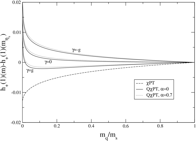
Figure 3: Dependence of $h_{+}(1)$ on the mass $m_{q}$ of the light spectator quark in Q$\chi$PT. For comparison, the $\chi$PT result from Randall and Wise (1993) is also shown (dashed line). The result has been normalized to unity for $m_{q}=m_{s}$. We have chosen $\mu_{0}=700\,\text{MeV}$ and $g^{2}=0.4$.

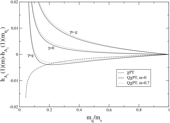
Figure 4: Dependence of $h_{A_{1}}(1)$ on the mass of the light spectator quark in Q$\chi$PT. The dashed line denotes the $\chi$PT result Randall and Wise (1993). The numerical values for the parameters are those used in Fig. (3).

The graphs are plotted against $m_{q}$ in units of the strange quark mass $m_{s}$ with $m_{q}/m_{s}=m^{2}/m_{\eta_{s}}^{2}$ where $m_{\eta_{s}}^{2}=2m_{K}^{2}$. The behavior of $h_{+}(1)$ in Q$\chi$PT is dominated at small $m$ by the $1/m^{2}$ pole that is non-existent in $\chi$PT. Lattice calculations of $h_{+}(1)$ El-Khadra et al. (2001) show a small downward trend for decreasing $m_{q}$ down to the chiral limit that is similar to the downward trend seen from the $\chi$PT calculation (dashed line). The same behavior (down to $m_{q}\approx 0.1m_{s}$) can also be seen for Q$\chi$PT for a certain choice of parameters (e.g., ${\gamma}$ positiv). The case of $h_{A_{1}}(1)$ is different as there is a pole at $m={\Delta}_{D}$ which is close to the physical pion mass. Here, both $D^{*}$ and $\pi$ can be on-shell and the decay $B\to D^{*}\pi$ becomes kinematically allowed. Lattice calculations of $h_{A_{1}}(1)$ Hashimoto et al. (2001) for $m_{q}=(0.6\dots 1)m_{s}$ show a small downward trend for decreasing $m_{q}$ similar to the downward trend seen from the $\chi$PT calculation [dashed line in Fig. (4)]. A similar trend down to $m_{q}\approx 0.2m_{s}$ can also be seen in the Q$\chi$PT calculation for a relatively large positiv value of ${\gamma}$.

Although the downward trend in the lattice data for the two cases seems significant as the statistical errors are highly correlated, the uncertainty is still relatively high (typically $\pm 0.01$) and the existing lattice data can be accommodated by a wide range of values for the parameters in the Q$\chi$PT Lagrangian.

Finally, we calculate the double ratios defined in Eqs. (4)–(6) using the results in Eqs. (33)–(35). We find

$${\mathcal{R}}_{+}=1+2{\delta}h_{+}(1),$$ (36)

$${\mathcal{R}}_{1}=1+2{\delta}h_{1}(1),$$ (37)

and

$${\mathcal{R}}_{A_{1}} = 1+\tilde{X}_{A_{1}}(\mu)$$ (38)

$$-\frac{ig^{2}}{3f^{2}}\left\{\mu_{0}^{2}\left[H_{5}({\Delta}_{B},-{\Delta}_{D})+H_{5}({\Delta}_{D},-{\Delta}_{B})-H_{5}({\Delta}_{D},-{\Delta}_{D})-H_{5}({\Delta}_{B},-{\Delta}_{B})\right]\right.$$

$$\left.\phantom{gggggg}-{\alpha}\left[H_{8}({\Delta}_{B},-{\Delta}_{D})+H_{8}({\Delta}_{D},-{\Delta}_{B})-H_{8}({\Delta}_{D},-{\Delta}_{D})-H_{8}({\Delta}_{B},-{\Delta}_{B})\right]\right\}$$

$$-\frac{2ig{\gamma}}{f^{2}}\left[G_{5}({\Delta}_{B},-{\Delta}_{D})+G_{5}({\Delta}_{D},-{\Delta}_{B})-G_{5}({\Delta}_{D},-{\Delta}_{D})-G_{5}({\Delta}_{B},-{\Delta}_{B})\right]$$

$$\rightarrow 1+\tilde{X}_{A_{1}}(\mu)-\frac{1}{(4\pi f)^{2}}\left(\frac{2g^{2}\mu_{0}^{2}}{9m^{2}}-\left[\frac{2g^{2}{\alpha}}{9}-\frac{4g{\gamma}}{3}\right]\log\frac{m^{2}}{\mu^{2}}\right)\left({\Delta}_{B}-{\Delta}_{D}\right)^{2}$$

$$+{\mathcal{O}}(\{{\Delta}_{B},{\Delta}_{D}\}^{3}),$$

where $\tilde{X}_{A_{1}}(\mu)$ is the counter term associated with ${\mathcal{R}}_{A_{1}}$.

VI Conclusions

Knowledge of the $B^{(*)}\to D^{(*)}$ form factors at the zero-recoil point is crucial to extract the value of $V_{cb}$ from experiment. In the limit that the heavy quarks are infinitely heavy HQET predicts that the form factors $h_{+}$, $h_{A_{1}}$, and $h_{1}$ are equal, $h_{+}(1)=h_{A_{1}}(1)=h_{1}(1)=\xi(1)$. The formally dominant correction due to breaking of heavy quark symmetry comes from the inclusion of a ${\mathcal{O}}(1/M)$ dimension-three operator in the Lagrangian that leads to hyperfine-splitting between the heavy pseudoscalar and vector mesons. These leading order corrections are ${\mathcal{O}}(\{{\Delta}_{B},{\Delta}_{D}\}^{2}$ as required by Luke’s theorem.

Recent lattice simulations using the quenched approximation of QCD have made a big step forward in determining these zero-recoil form factors. Presently, however, the simulations use light quark masses that are much heavier than the physical ones and therefore rely on a chiral extrapolation down to the physical quark masses. In this paper we have calculated the dominant corrections to the form factors $h_{+}$, $h_{A_{1}}$, and $h_{1}$ in Q$\chi$PT and determined the non-analytic dependence on the light quark masses via the light meson masses $m_{qq}$. Using these results, instead of the $\chi$PT calculation, to extrapolate the QQCD lattice measurements of these form factors down to the physical pion mass should give a more reliable estimate of the errors associated with the chiral extrapolation.

We have also calculated the corrections to certain double ratios that are used in lattice QCD calculations of the decay $B\to D^{*}$.

Appendix A Integrals

We list the functions $H_{1}$, $H_{2}$, $F_{1}$, $H_{5}$, $H_{8}$, and $G_{5}$ even though some of them have appeared in the literature before Boyd and Grinstein (1995b, a). Here, $m=m_{qq}$ is the mass of the $q\bar{q}$ light meson in the loop where $q=u$, $d$, or $s$ is the light (spectator) quark content of the heavy mesons. We have used dimensional regularization with the $\overline{\text{MS}}$ scheme, where $1/{\epsilon}^{\prime}\equiv 1/{\epsilon}-{\gamma}_{E}+\log 4\pi+1$. At the end we set $1/{\epsilon}^{\prime}=0$. As a shorthand we have defined the function

$$R(x)=\sqrt{x^{2}-1}\log\left(\frac{x-\sqrt{x^{2}-1+i{\epsilon}}}{x+\sqrt{x^{2}-1+i{\epsilon}}}\right),$$ (39)

which occurs frequently. We also need its derivative $dR/dx$ given by

$$R^{\prime}(x)=\frac{x}{x^{2}-1}R(x)-2.$$ (40)

For the calculation of the wavefunction renormalization contribution we need the derivatives of the loop integrals for the diagrams in Fig. (1):

$$H_{1}({\Delta})=\frac{i}{16\pi^{2}}\left[\log\frac{m^{2}}{\mu^{2}}-\frac{1}{{\epsilon}^{\prime}}-1-R^{\prime}\left(\frac{{\Delta}}{m}\right)\right],$$ (41)

$$H_{2}({\Delta}) = \frac{i}{16\pi^{2}}\left[\frac{16}{3}{\Delta}^{2}-\frac{10}{3}m^{2}+2(m^{2}-{\Delta}^{2})\left(\!\log\frac{m^{2}}{\mu^{2}}-\frac{1}{{\epsilon}^{\prime}}\right)+\frac{4}{3}{\Delta}mR\left(\frac{{\Delta}}{m}\right)\right.$$ (42)

$$\left.\phantom{dddddd}+\left(\frac{2}{3}{\Delta}^{2}-\frac{5}{3}m^{2}\right)R^{\prime}\left(\frac{{\Delta}}{m}\right)\right],$$

and

$$F_{1}({\Delta}) = \frac{i}{16\pi^{2}}\left[\frac{10}{3}{\Delta}^{2}-\frac{4}{3}m^{2}+\left(m^{2}-2{\Delta}^{2}\right)\left(\!\log\frac{m^{2}}{\mu^{2}}-\frac{1}{{\epsilon}^{\prime}}\right)+\frac{4}{3}{\Delta}mR\left(\frac{{\Delta}}{m}\right)\right.$$ (43)

$$\left.\phantom{dddddd}+\frac{2}{3}({\Delta}^{2}-m^{2})R^{\prime}\left(\frac{{\Delta}}{m}\right)\right].$$

For the loop-integrals of the vertex corrections one finds

$$H_{5}({\Delta},{\tilde{\Delta}})=\frac{i}{16\pi^{2}}\left(\log\frac{m^{2}}{\mu^{2}}-\frac{1}{{\epsilon}^{\prime}}-1-\frac{m}{{\Delta}-{\tilde{\Delta}}}\left[R\left(\frac{{\Delta}}{m}\right)-R\left(\frac{{\tilde{\Delta}}}{m}\right)\right]\right),$$ (44)

$$H_{8}({\Delta},{\tilde{\Delta}}) = \frac{i}{16\pi^{2}}\left(\left[2m^{2}-\frac{2}{3}({\Delta}^{2}+{\Delta}{\tilde{\Delta}}+{\tilde{\Delta}}^{2})\right]\left(\log\frac{m^{2}}{\mu^{2}}-\frac{1}{{\epsilon}^{\prime}}\right)+\frac{16}{9}({\Delta}^{2}+{\Delta}{\tilde{\Delta}}+{\tilde{\Delta}}^{2})\right.$$ (45)

$$\left.\phantom{dddddd}-\frac{10}{3}m^{2}+\frac{m(5m^{2}-2{\tilde{\Delta}}^{2})}{3({\Delta}-{\tilde{\Delta}})}R\left(\frac{{\tilde{\Delta}}}{m}\right)-\frac{m(5m^{2}-2{\Delta}^{2})}{3({\Delta}-{\tilde{\Delta}})}R\left(\frac{{\Delta}}{m}\right)\right),$$

and

$$G_{5}({\Delta},{\tilde{\Delta}}) = \frac{i}{16\pi^{2}}\left(\frac{10}{9}({\Delta}^{2}+{\Delta}{\tilde{\Delta}}+{\tilde{\Delta}}^{2})-\frac{4}{3}m^{2}+\left[m^{2}-\frac{2}{3}({\Delta}^{2}+{\Delta}{\tilde{\Delta}}+{\tilde{\Delta}}^{2})\right]\left(\!\log\frac{m^{2}}{\mu^{2}}-\frac{1}{{\epsilon}^{\prime}}\right)\right.$$ (46)

$$\left.\phantom{dddddd}+\frac{2m({\Delta}^{2}-m^{2})}{3({\Delta}-{\tilde{\Delta}})}R\left(\frac{{\Delta}}{m}\right)-\frac{2m({\tilde{\Delta}}^{2}-m^{2})}{3({\Delta}-{\tilde{\Delta}})}R\left(\frac{{\tilde{\Delta}}}{m}\right)\right).$$

References

Manohar and Wise (2000)
A. V. Manohar and
M. B. Wise,
Cambridge Monogr. Part. Phys. Nucl. Phys. Cosmol.
10, 1 (2000).
Czarnecki (1996)
A. Czarnecki,
Phys. Rev. Lett. 76,
4124 (1996),
eprint [http://arXiv.org/abs]hep-ph/9603261.
Luke (1990)
M. E. Luke,
Phys. Lett. B252,
447 (1990).
Briere et al. (2002)
R. A. Briere
et al. (CLEO), Phys.
Rev. Lett. 89, 081803
(2002), eprint [http://arXiv.org/abs]hep-ex/0203032.
Simone et al. (2000)
J. N. Simone
et al., Nucl. Phys. Proc. Suppl.
83, 334 (2000),
eprint [http://arXiv.org/abs]hep-lat/9910026.
El-Khadra et al. (2001)
A. X. El-Khadra,
A. S. Kronfeld,
P. B. Mackenzie,
S. M. Ryan, and
J. N. Simone,
Phys. Rev. D64,
014502 (2001),
eprint [http://arXiv.org/abs]hep-ph/0101023.
Hashimoto et al. (2001)
S. Hashimoto,
A. S. Kronfeld,
P. B. Mackenzie,
S. M. Ryan, and
J. N. Simone
(2001), eprint [http://arXiv.org/abs]hep-ph/0110253.
Kronfeld et al. (2002)
A. S. Kronfeld,
P. B. Mackenzie,
J. N. Simone,
S. Hashimoto,
and S. M. Ryan
(2002), eprint [http://arXiv.org/abs]hep-ph/0207122.
Randall and Wise (1993)
L. Randall and
M. B. Wise,
Phys. Lett. B303,
135 (1993),
eprint [http://arXiv.org/abs]hep-ph/9212315.
Boyd and Grinstein (1995a)
C. G. Boyd and
B. Grinstein,
Nucl. Phys. B451,
177 (1995a),
eprint [http://arXiv.org/abs]hep-ph/9502311.
Savage (2002)
M. J. Savage,
Phys. Rev. D65,
034014 (2002),
eprint [http://arXiv.org/abs]hep-ph/0109190.
Morel (1987)
A. Morel, J.
Phys. (France) 48, 1111
(1987).
Sharpe (1992)
S. R. Sharpe,
Phys. Rev. D46,
3146 (1992),
eprint [http://arXiv.org/abs]hep-lat/9205020.
Bernard and
Golterman (1992a)
C. W. Bernard and
M. F. L. Golterman,
Phys. Rev. D46,
853 (1992a),
eprint [http://arXiv.org/abs]hep-lat/9204007.
Bernard and
Golterman (1992b)
C. W. Bernard and
M. Golterman,
Nucl. Phys. Proc. Suppl. 26,
360 (1992b).
Golterman (1994)
M. F. L. Golterman,
Acta Phys. Polon. B25,
1731 (1994),
eprint [http://arXiv.org/abs]hep-lat/9411005.
Booth (1995)
M. J. Booth,
Phys. Rev. D51,
2338 (1995),
eprint [http://arXiv.org/abs]hep-ph/9411433.
Sharpe and Zhang (1996)
S. R. Sharpe and
Y. Zhang,
Phys. Rev. D53,
5125 (1996),
eprint [http://arXiv.org/abs]hep-lat/9510037.
Falk and Neubert (1993)
A. F. Falk and
M. Neubert,
Phys. Rev. D47,
2965 (1993),
eprint [http://arXiv.org/abs]hep-ph/9209268.
Isgur and Wise (1989)
N. Isgur and
M. B. Wise,
Phys. Lett. B232,
113 (1989).
Isgur and Wise (1990)
N. Isgur and
M. B. Wise,
Phys. Lett. B237,
527 (1990).
Booth (1994)
M. J. Booth
(1994), eprint [http://arXiv.org/abs]hep-ph/9412228.
Witten (1979)
E. Witten,
Nucl. Phys. B156,
269 (1979).
Veneziano (1979)
G. Veneziano,
Nucl. Phys. B159,
213 (1979).
Boyd and Grinstein (1995b)
C. G. Boyd and
B. Grinstein,
Nucl. Phys. B442,
205 (1995b),
eprint [http://arXiv.org/abs]hep-ph/9402340.