Simulations of Alice Electrodynamics on a Lattice

Abstract

In this paper we present results of numerical simulations and some (analytical) approximations of a compact $U(1)\ltimes\mathbb{Z}_{2}$ lattice gauge theory, including an extra bare mass term for Alice fluxes. The subtle interplay between Alice fluxes and (Cheshire) magnetic charges is analysed. We determine the phase diagram and some characteristics of the model in three and four dimensions. The results of the numerical simulations in various regimes, compare well with some analytic approximations.

1 Introduction

In this paper we investigate a lattice version of Alice electrodynamics (LAED). Alice electrodynamics (AED) is a gauge theory with gauge group $U(1)\ltimes\mathbb{Z}_{2}\sim O(2)$, in other words a minimally non-abelian extension of ordinary electrodynamics [1]. The nontrivial $\mathbb{Z}_{2}$ transformation reverses the direction of the electric and magnetic fields and the sign of the charges. This means that in Alice electrodynamics charge conjugation symmetry is gauged. However, as this non-abelian extension is discrete, it only affects electrodynamics through certain global (topological) features, such as the appearance of Alice fluxes (or vortices) and Cheshire charges [2]. The topological structure of $U(1)\ltimes\mathbb{Z}_{2}$ differs from that of $U(1)$ in a few subtle points. Firstly, AED allows topologically stable vortices since $\Pi_{0}(U(1)\ltimes\mathbb{Z}_{2})=\mathbb{Z}_{2}$, these will be referred to as Alice fluxes. Note that in this theory this flux is coëxisting with the unbroken $U(1)$ of electromagnetism and therefore it is not an “ordinary” magnetic flux. Secondly, just as the compact $U(1)$ gauge theory, AED also contains magnetic monopoles, because $\Pi_{1}(U(1)\ltimes\mathbb{Z}_{2})=\mathbb{Z}$. We note however, that due to the fact that the $\mathbb{Z}_{2}$ and the $U(1)$ part of the gauge group do not commute, magnetic charges of opposite sign belong to the same topological class. The aim of this paper is to get an understanding of the phase diagram in a simple lattice version of Alice electrodynamics but which does contain both monopoles and Alice fluxes. We do so by simulations and some analytic approximations.

The paper is organised as follows. In section 2 we specify the lattice model in detail. In section 3 we give the numerical results we obtained for the phase diagrams of the model in dimensions three and four. In section 3 we present some analytic approximations related to the phase diagram and other measurable quantities. In the final section we summarise the results and draw conclusions.

2 Lattice Alice Electrodynamics

In this section we introduce a specific LAED model. First we explain the different terms that appear in the action and then we discuss how magnetic monopoles and instantons are realized and can be measured. Finally we say a few things about the computational implementation of the model.

2.1 The action

Alice phases can be generated by spontaneously breaking $SU(2)$ to $U(1)\ltimes\mathbb{Z}_{2}$. In this case it is clear that Alice loops, monopoles and Cheshire charges may arise as regular classical finite energy solutions. In the study presented here we restrict ourselves to compact $U(1)\ltimes\mathbb{Z}_{2}$ gauge theory with an extra bare mass term for the Alice fluxes. Our lattice formulation of the theory allows for the formation of Alice fluxes and magnetic monopoles. The action we will use is given by:

$$I=\frac{1}{g^{2}}\sum_{plaquettes}\{-\Re(Tr(U_{1}U_{2}U_{3}^{\dagger}U_{4}^{\dagger}))+m_{f}P_{f}\}~{}.$$ (1)

The first part represents the normal Wilson [3] plaquette action for the gauge theory. The second term is the extra bare mass term for the $\mathbb{Z}_{2}$ fluxes in the model. $P_{f}$ is a functional of the $\mathbb{Z}_{2}$ degrees of freedom which, when evaluated on a plaquette, equals one if the plaquette is pierced by a $\mathbb{Z}_{2}$ flux, and equals zero if not. The parameter $m_{f}$ is the extra bare mass (in three dimensions) or tension (in four dimensions) for the Alice flux.

In principle one can also add an extra bare monopole mass term to the action. We have refrained from doing so because it is computationally much more involved and because we can realize all four phases in the model without this term (see table 1). To define suitable link variables for LAED we use the fact that compact $U(1)\ltimes\mathbb{Z}_{2}$ can be conveniently embedded in $SU(2)$, leading to:

$$U_{\nu}(x)=e^{iA_{\nu}(x)\tau_{3}}\tau_{1}^{a_{\nu}(x)}~{},$$ (2)

with $a_{\nu}(x)\in\{0,1\}$ and $A_{\nu}(x)\in\langle-\pi,\pi]$. Thus $a_{\nu}$ represents the $\mathbb{Z}_{2}$ gauge variable and $A_{\nu}$ the compact $U(1)$ gauge variable of the theory. We say that, if $a_{\nu}(x)=1$ a $\mathbb{Z}_{2}$-sheet in 3D, or a $\mathbb{Z}_{2}$-volume in 4D, crosses the link, implying that the $\mathbb{Z}_{2}$-sheets live on the dual lattice. These $\mathbb{Z}_{2}$-sheets can, of course, be moved around by local $\mathbb{Z}_{2}$ gauge transformations. A gauge transformation of the links is given by:

$$U_{\nu}(x)\to\Omega(x)U_{\nu}(x)\Omega(x+\hat{\nu})^{\dagger}~{},$$ (3)

with $\Omega(x)=e^{i\Sigma_{\nu}(x)\tau_{3}}\tau_{1}^{\sigma_{\nu}(x)}$, where $\sigma_{\nu}(x)\in\{0,1\}$ and $\Sigma_{\nu}(x)\in\langle-\pi,\pi]$.
The boundaries of the $\mathbb{Z}_{2}$-sheets, however, cannot be moved around by local $\mathbb{Z}_{2}$ gauge transformations, this in analogy with the endpoints of Dirac strings (being magnetic monopoles) in the compact $U(1)$ gauge theory. This is exactly what one should expect, since the boundaries of the $\mathbb{Z}_{2}$-sheets are closed Alice flux loops, which are physical objects carrying energy. Bearing this in mind it is easy to locate the Alice fluxes, namely by just counting the number of $\mathbb{Z}_{2}$-sheets crossing the links of a plaquette. If an even number of $\mathbb{Z}_{2}$-sheets crosses the links of the plaquette, then no Alice flux pierces the plaquette, but if an odd number does, then that means that an Alice flux does pierce the plaquette. This observation allows one to define the $P_{f}$ operator, which applied to a plaquette measures the presence of an Alice flux,

$$P_{f}=\frac{1}{2}(1-(-1)^{\sum_{i=1}^{4}a_{i}})~{},$$ (4)

where the four $a_{i}$ summed over belong to links $U_{1}$, $U_{2}$, $U_{3}$ and $U_{4}$, bounding a single plaquette. Equations (1), (2) and (4) define our LAED model.

2.2 The problem of locating monopoles (or instantons)

In this model of LAED in four dimensions, there are magnetic monopoles, in three dimensions these appear as instantons. There are a few intricacies in detecting them compared to the usual compact $U(1)$ lattice gauge theory. In this section we will explain under what circumstances and how we can detect a monopole/instanton in LAED. As our model of LAED has a lot of similarities with compact $U(1)$ lattice gauge theory, we try to use these similarities in determining the monopole content of a configuration.

Let us first consider the case that there are no Alice fluxes present. Clearly, this corresponds to the limit of an infinitely large mass, $m_{f}$, for the flux. In this case there may still be closed $\mathbb{Z}_{2}$ surfaces, but these surfaces are not physical and can be moved around by making suitable local $\mathbb{Z}_{2}$ transformations. Suppose we want to determine the monopole content of a specific cube in such a configuration. We would like to see if a Dirac string ends in the cube, just as one does for compact $U(1)$ lattice gauge theory. We distinguish two cases, the first where no $\mathbb{Z}_{2}$-sheet crosses the cube of interest and the second where one or more $\mathbb{Z}_{2}$-sheets do cross the cube.

In the first case we determine the monopole content of the cube just as in compact $U(1)$ lattice gauge theory. In the second case we should find a new or more general definition due to the presence of the $\mathbb{Z}_{2}$-sheets. Bearing in mind that a monopole is a physical object which cannot be moved around by gauge transformations, one may use local $\mathbb{Z}_{2}$ gauge transformations to gauge the $\mathbb{Z}_{2}$-sheets away from the cube of interest. After this procedure we can again determine the monopole content by the methods of compact $U(1)$ lattice gauge theory.

$\mathbb{Z}_{2}$-sheets can be gauged out of the cube of interest in several different ways. One would expect this not to make any difference to the outcome of the measurement of the monopole charge of the cube of interest, but it does! As we mentioned in the introduction, monopoles of opposite sign belong to the same topological class. For the measurement of the monopole charge of a single cube this means that one cannot distinguish between positive and negative charges. To see that this is the case, let us consider a cube which is not intersected by a $\mathbb{Z}_{2}$-sheet. If one performs a ’global’ $\mathbb{Z}_{2}$ gauge transformation to all the links of this cube, this has the same effect as pulling a $\mathbb{Z}_{2}$-sheet through the cube; all the $U(1)$ degrees of freedom change sign, since $\tau_{1}e^{iA\tau_{3}}\tau_{1}=e^{-iA\tau_{3}}$, see equation (3). Obviously this means that the outcome of the measurement of the magnetic charge of the cube changes sign. Hence only the absolute value of the magnetic charge is a locally gauge invariant quantity, i.e. an observable.

Next we consider the situation where fluxes are present. Now we have two different type of cubes, cubes which are pierced by a flux and cubes which are not. The latter are obviously equivalent to the cubes we just discussed. Thus at this point we may restrict our considerations to cubes which are pierced by fluxes. The statement is, that for a cube which is pierced by a flux, the notion of a gauge invariant magnetic charge breaks down completely. Let us explain why this is the case.

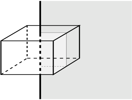
Figure 1: A cube that is pierced by a flux which is the boundary of a $\mathbb{Z}_{2}$-sheet.

If an Alice flux pierces through a cube, it is obviously not possible to gauge the $\mathbb{Z}_{2}$-sheet out of the cube. In figure 1 we depicted a cube pierced by a flux and the $\mathbb{Z}_{2}$-sheet connected to the flux. If one tries to define Dirac strings through the plaquettes bounding the cube of interest one gets into all sorts of trouble. For the plaquettes where no flux pierces through one can up to a sign determine the (real magnetic flux through the) Dirac string. This sign problem seems to be a minor one, as it appears to be for the monopole charge itself, but that is not true, because there is a separate sign ambiguity for the Dirac strings through each of the plaquettes and not just a single overall sign, as was the case for a cube not pierced by a flux. This means that in such a cube, even the absolute value of the net magnetic charge is not an invariant quantity.

Yet another problem arises if one wants to define the Dirac string through a plaquette which is pierced by a flux, because an odd number of $\mathbb{Z}_{2}$-sheets cross the links bounding the plaquette. The problem basically follows directly from Alice electrodynamics itself, where if one sweeps a $\mathbb{Z}_{2}$-sheet through a $U(1)$ link field, this will change sign. So even the sign of the individual $U(1)$ link variables is not defined uniquely on a plaquette which is intersected by an odd number of sheets, even if one looks only at that particular plaquette. This obstruction to defining the magnetic flux through such a plaquette, is just a manifestation of what is generally called the obstruction to globally define a $U(1)$ charge in the presence of an Alice flux in Alice electrodynamics.

However not all is lost. The previous discussion only shows that it is impossible to determine the magnetic charge of a cube, or more general of a volume, whose bounding surface is pierced by a flux. There is however no problem in determining the magnetic charge of a volume which contains a loop of flux not crossing the boundary.

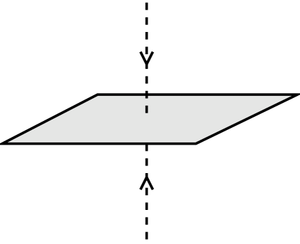
Figure 2: This figure shows an Alice loop with its $\mathbb{Z}_{2}$-sheet. The $\mathbb{Z}_{2}$-sheet is pierced by a Dirac string, which changes sign/direction once it passes the $\mathbb{Z}_{2}$-sheet. In this configuration the Alice loop carries a magnetic Cheshire charge.

To see this consider the configuration given in figure 2. A configuration is shown of an Alice loop and a Dirac string piercing the $\mathbb{Z}_{2}$-sheet bounded by the Alice loop. This figure demonstrates, that an Alice loop configuration is capable of carrying a magnetic charge. We note that there is no Dirac string coming from the flux itself (this is actually possible and even necessary for the unit charged Alice loop). Remember that we are, for plaquettes not pierced by a flux, able to determine the Dirac string up to a sign. We also note that any attempt to measure the location of the monopole will fail. It looks like that the cube where the the Dirac string pierces the $\mathbb{Z}_{2}$-sheet does contain a magnetic charge, but as the position of the sheet is gauge dependent this is just a gauge illusion. Yet, drawing a closed 2-surface around the loop there is a gauge invariant quantity of magnetic flux emanating from that surface, i.e. there is magnetic charge inside. This magnetic charge is present, not as a localised or even localiseable quantity, but rather as a global property carried by a closed Alice loop as a whole, in which case one speaks of a magnetic “Cheshire” charge. And indeed, although one can determine the magnetic charge carried by the Alice loop as a whole, one can not assign this magnetic charge to any of the cubes inside the volume containing the loop. These nonlocaliseable charges may in the continuum even be energetically favoured, as we showed in [4], ’t Hooft Polyakov monopoles may decay in their Cheshire versions.

We conclude, that once we enter a phase where there are very many Alice fluxes around, detecting and localising magnetic charge gets a hairy business. The only useful thing one may still do, is to measure the fraction of monopole carrying cubes of the number of cubes not pierced by an Alice flux. In view of these observations, when in the following we talk about the monopole density, we mean the average absolute charge per unpierced cube and when we talk about flux density we mean the fraction of plaquettes pierced by an Alice flux, i.e. $\langle P_{f}\rangle$, unless stated otherwise.

2.3 Implementation of the model

Although formula (2) suggests that we should implement LAED using (Pauli) matrices we have not done so. Instead, we exploited the fact that the structure of our $U(1)\ltimes\mathbb{Z}_{2}$ gauge theory is very close to that of the compact $U(1)$. The only effect of the $\mathbb{Z}_{2}$ degrees of freedom is the appearance of Alice fluxes and $\mathbb{Z}_{2}$-sheets. If there are an odd number of $a$ variables equal to one in a plaquette, then the plaquette is pierced by a $\mathbb{Z}_{2}$ flux and the first term in the action is always zero irrespective of the values of the $A$ fields. This can be understood as a consequence of the fact that the $U(1)$ symmetry is globally frustrated in the presence of an Alice flux. If, in the contrary, there are an even or zero number of $a$ variables equal to one in a plaquette, the $a$ variables can be gauged away, changing only the sign of some of the $A$ fields and the action is just the action of compact $U(1)$. In view of these observations, we have for our simulations used the following simple action, which is equivalent to the action of formula (1), but does not require any matrix calculations.

$$I=\frac{1}{g^{2}}\sum_{plaquettes}\{-(1-P_{f})\cos{\tilde{F}}+m_{f}P_{f}\}~{},$$ (5)

where $\tilde{F}$ is the $F$ of $U(1)$ after the $\mathbb{Z}_{2}$ fields have been gauge transformed out of the plaquette, which is always possible if $P_{f}=0$.

We have investigated this model, using a combination of a Monte Carlo method for the $A_{\nu}(x)$ variables, and a heat bath method for the $a_{\nu}(x)$ variables. We examined the model on a periodic hyper cubic lattice of size $10^{d}$, where d is the dimension. Although we will not go into detail on the order of the phase transitions we mention that it has been suggested [5], that the order, oddly enough, would depend on the imposed boundary conditions.

Our LAED model contains a pure compact $U(1)$ and a $\mathbb{Z}_{2}$ gauge theory in different limits of the model. In the limit of $m_{f}\to\infty$ the model is equal to pure compact $U(1)$ gauge theory. In the limit of $g^{2}\to\infty$ while keeping $m_{f}/g^{2}$ finite the model is equal to $\mathbb{Z}_{2}$ gauge theory. Before we proceed we like to mention a few things about the $\mathbb{Z}_{2}$ gauge theory to avoid confusion later on. In $\mathbb{Z}_{2}$ gauge theory there is only one parameter, in the $\mathbb{Z}_{2}$ limit of our model this parameter is $m_{f}/g^{2}$. Normally, the $\mathbb{Z}_{2}$ gauge theory is only studied for positive values of its parameter. However, in our situation we are also interested in the region where $m_{f}/g^{2}$ becomes negative. In the pure $\mathbb{Z}_{2}$ gauge theory the region of positive and negative values of the parameter form a mirror image of each other. Note that this mirror map is different from the usual duality that is also present in $\mathbb{Z}_{n}$ type gauge theories. This mirror symmetry holds, at least, for a hyper cubic lattice, where one may map the negative coupling side on the positive side if one replaces “fluxes” by “no-fluxes” in every sense. So “no-fluxes” are the places where “no flux” pierces through a plaquette, i.e. they are the holes in the flux condensate. The model can equally well be described by either of the two objects. This mirror symmetry follows from the fact that for a hyper cubic lattice both objects, fluxes and no-fluxes, form closed loops in three dimensions and closed surfaces in four dimensions. This shows that the regions of positive values and negative values of $m_{f}/g^{2}$ are can be naively mapped onto each other. As we will show, in LAED the Alice mirror symmetry is broken by the interactions with the $U(1)$ gauge fields for finite values of $g^{2}$.

3 The phase diagram in three and four dimensions

In this section we present various numerical results for the LAED model. Because we have two types of topological objects in the theory, which may or may not condense, one may in principle expect four phases. It is quite easy to anticipate where in the parameter space the four phases could occur, as we have indicated in table 1.

$m_{f}$ small $m_{f}$ large $g^{2}$ small Fluxes No Condensate $g^{2}$ large Fluxes and Monopoles/ Monopoles/ Instantons Instantons

Table 1: The four phases of LAED.

In figure 3(a) we have plotted the flux density and the monopole density in four dimensions. It is clear that various interesting transitions do occur. Using a hysteresis type of analysis we could determine the order of these transitions, and we found that all but one, are of first order. Only the transition from the phase with only Alice fluxes condensed, to the phase where both Alice fluxes and monopoles are condensed, is different. In fact, it does appear not to be a phase transition at all, but rather a crossover phenomenon, see also section 4.4 and the discussion in section 4.5.

In figure 3(b) we have plotted some contours for the Alice flux and monopole densities. The curves indicate where the first order phase transitions take place, but also show the change of the first order monopole transition if no fluxes are condensed, to the crossover monopole transition if fluxes are condensed.

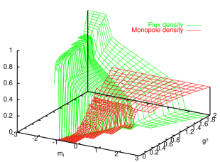
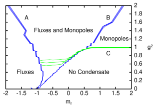
(a) (b)

Figure 3:
(a): The 4-dimensional flux and the monopole densities are plotted as a function of $m_{f}$ and $g^{2}$. The four different phases of table 1 can be clearly distinguished.
(b): A plot of some specific monopole and the Alice flux density contours in four dimensions. We identify the four phases of the model. The lines denoted $B$ mark the transition involving the Alice fluxes, where to the left of $B$ the fluxes are condensed. The lines $A$ correspond to a second phase transition involving the fluxes. The lines $C$ denote the monopole transition, notice the splitting of the height lines once the Alice fluxes are condensed.

Note that in figures 3(a) and 3(b) we have only plotted the monopole density up to the ’second’ flux density transition, line A in figure 3(b), where the flux density jumps to about one and only very few cubes (if any) are left where no flux pierces through, making the fluctuations for the monopole measurement very large.

Though in our limited model we find all of the anticipated four phases, each characterised by some condensate, we do not find all possible transitions from one phase to another. There is apparently no transition from the phase with condensed monopoles and no fluxes to the phase with condensed fluxes and no monopoles.

In appropriate limits of the model we recover the results for the lattice gauge theories of compact $U(1)$ and $\mathbb{Z}_{2}$ separately, consistent with equation (5). The pure $U(1)$ gauge theory arises in the limit of $m_{f}\to\infty$, where the Alice fluxes are suppressed and the only feature reminiscent of the $\mathbb{Z}_{2}$ part of the gauge theory are pure $\mathbb{Z}_{2}$ gauge transformations, which of course do not affect any of the physics. In this limit we therefore expect only the transition corresponding to monopole condensation. The pure $\mathbb{Z}_{2}$ gauge theory arises in the limit of $g^{2}\to\infty$, while keeping $m_{f}/g^{2}$ finite, which is usually only studied with $m_{f}/g^{2}\geq 0$. We verified that the limiting behaviours of the results of our simulations are in agreement with the known results of the $\mathbb{Z}_{2}$ and $U(1)$ gauge theories [6, 7, 8, 9], see also [10] and references therein.

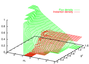
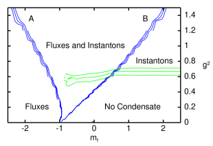
(a) (b)

Figure 4:
(a): The 3-dimensional flux and instanton densities are plotted as a function of $m_{f}$ and $g^{2}$. The four different phases of table 1 are clearly distinguishable.
(b): In this figure we plotted some specific height lines of the instanton and the Alice flux density in three dimensions. We identify the four phases of the model. Line $B$ is the condensation line of the Alice fluxes, to the left of it the fluxes are condensed. Line $A$ is a second phase transition. In comparison with figure 3(b) there is no line $C$. In three dimensions the instanton condensation is always a crossover.

In figure 4(a) we plotted the results for the instanton and Alice flux density in three dimensions. Also in this case we encounter all four phases of the theory, but the transitions are of different order. The instanton condensation is always a crossover and the flux condensation appears to be of second order, which it certainly should be in the $\mathbb{Z}_{2}$ gauge theory limit [7]. We did not determine the order of the flux condensation for small $g^{2}$.

In figure 4(a) the transition for small values of $g^{2}$ appears to become a first order phase transition, but this is mainly due to the fact that we use $m_{f}$ and $g^{2}$ to parameterise the model, whereas the, in some sense more natural, choice of $(m_{f}+1)/g^{2}$ and $1/g^{2}$ could give a different picture, which is also true for the four dimensional case. We will come back to this point in section 4.5.

In figure 4(b) we, just as in figure 3(b), plotted specific height lines of the instanton and Alice flux density. These lines show the location of the Alice flux phase transitions and divide the parameter space up in the four different regions linked to the phases. Again in the $U(1)$ and $\mathbb{Z}_{2}$ limit we recover the results of these pure gauge theories separately.

In three dimensions the flux density becomes very high before the second phase transition of the fluxes, line A in figure 4(b), occurs and consequently the fluctuations of the instanton density measurements become very large in a larger region.

4 Analytic and other approximations

LAED contains both pure compact $U(1)$ and $\mathbb{Z}_{2}$ gauge theory. As both of these theories have been studied thoroughly over the years, our aim is not to make estimates for these models, but rather to treat their (numerical) results as known and focus on the interaction of these two models in LAED. To this end we give (analytical) approximations of some characteristic quantities of the model. We subsequently discuss the average action of unpierced plaquettes, the flux condensation lines, the contours of constant flux density in the region between the two flux condensation lines $A$ and $B$ and the monopole/instanton density. We conclude this section with a brief discussion of the approximations we made.

4.1 The average action of unpierced plaquettes

To approximate the average action per unpierced plaquette, $-\langle\cos{\tilde{F}}\rangle$, we split the parameter space of the model into two regions, a region where the $\mathbb{Z}_{2}$ fluxes do not condense and the region where they do.

In the region where the $\mathbb{Z}_{2}$ fluxes do not condense we approximate the theory by a pure U(1) gauge theory (in the present context considered to be given) and $-\langle\cos{\tilde{F}}\rangle$ is approximated accordingly, i.e. we ignore the effect which the few Alice fluxes have, that may be present. In the region where the fluxes do condense and the flux density is large, we approximate the average action of unpierced plaquettes by the average action of a single plaquette. The $U(1)$ link variables are irrelevant to plaquettes pierced by a flux, as follows from formula (5). In the limit of a high flux density the plaquettes which are not pierced by a flux become isolated in the sense that the value of the $U(1)$ degrees of freedom have almost no effect on the surrounding plaquettes. Thus we can approximate $-\langle\cos{\tilde{F}}\rangle$ in the condensed phase by:

$$\langle\cos{\tilde{F}}\rangle\approx\frac{\int^{2\pi}_{0}\frac{d\tilde{F}}{2\pi}\cos{\tilde{F}}e^{\frac{\cos{\tilde{F}}}{g^{2}}}}{\int^{2\pi}_{0}\frac{d\tilde{F}}{2\pi}e^{\frac{\cos{\tilde{F}}}{g^{2}}}}=\frac{I_{1}(\frac{1}{g^{2}})}{I_{0}(\frac{1}{g^{2}})}~{},$$ (6)

where the functions $I_{0}$ and $I_{1}$ are modified Bessel functions.

The difference between these two limits, the single plaquette and the $U(1)$ limit, vanishes for large $g^{2}$. In four dimensions, for small $g^{2}$, the fraction of pierced fluxes typically is very large in the flux condensed phase. Thus we may expect that the two limits describe the model for any value of $g^{2}$. In three dimensions there is no such jump in the flux density and we expect an intermediate region, for small $g^{2}$, to be present.

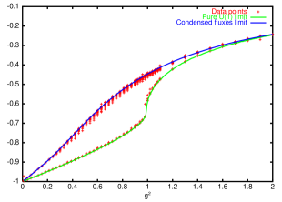
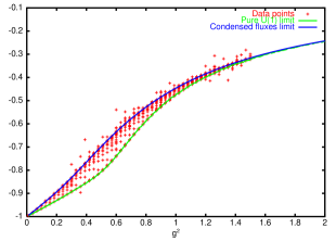
(a) (b)

Figure 5:
(a): The average plaquette action $-\langle\cos{\tilde{F}}\rangle$ in four dimensions. All the data points, i.e. including those corresponding to different values of $m_{f}$ and $g^{2}$, lie either on the pure $U(1)$ line or (almost) on the approximation for condensed fluxes phase. The division is so clear due to the strong first order $\mathbb{Z}_{2}$ transition, i.e. in the flux condensed phase the flux density is fairly high for small $g^{2}$.
(b): The average plaquette action $-\langle\cos{\tilde{F}}\rangle$ in three dimensions. Here the transition from the one region to the other is much more smooth, because the $\mathbb{Z}_{2}$ transition in three dimensions is only of second order, also the pure $U(1)$ result deviates much less from the flux condensed limit. The points outside the region between the two limits are points where the flux density is very high, implying that the fluctuations become very large.

In figure 5(a) we plotted $-\langle\cos{\tilde{F}}\rangle$ as a function of $g^{2}$ in four dimensions. We see that the data splits up into two lines. Part of the data points lie on the pure $U(1)$ line while the other part lies (almost) on the single plaquette line. This strict separation of the data points in these two sets is due to the strong first order behaviour of the $\mathbb{Z}_{2}$ flux condensation for small $g^{2}$. We see that each point is very well described by either the first or the second approximation indeed.

In figure 5(b) we plotted $-\langle\cos{\tilde{F}}\rangle$ as a function of $g^{2}$ in three dimensions. The two approximations now generate the boundaries between which the data points lie. The fact that there is no clear division of the data in two sets in three dimensions, is due to the fact that the $\mathbb{Z}_{2}$ phase transition is of second order. The flux density grows gradually across the transition region. That points appear also outside the region bounded by the two approximations is due to very large fluctuations when the flux density is high, i.e. when there are a small number of unpierced plaquettes.

4.2 The condensation lines of the Alice fluxes

To approximate the location of the Alice flux condensation lines in the parameter space of the model we make use of an action versus entropy argument. The weight factor of a configuration is determined by $e^{S-I}$. The important quantity is the relative weight factor, $e^{\Delta S-\Delta I}$, between configurations. Assuming that $S-I$ of the object that condenses, is additive with respect to the so called background, we find that $\Delta S-\Delta I=S_{object}-I_{object}$. Now typically the location of the critical point can be approximated by $I_{object}=S_{object}$.

As we saw in figures 3(b) and 4(b) there are two flux condensation lines in LAED. In the $\mathbb{Z}_{2}$ gauge theory these are just each other mirror image. For finite $g^{2}$ this symmetry between the two condensation lines is broken due to the interactions with the $U(1)$ fields. We may still compare them, in the sense that at the first transition line, B, the fluxes condense, while at the other, A, the “no-fluxes” condense. The coupling between the $\mathbb{Z}_{2}$ and the $U(1)$ fields manifests itself as follows: if a flux is created then a piece of the $U(1)$ fields is “eaten” away, in the sense that the $U(1)$ fields become irrelevant because they are projected out and do not affect the action of the plaquettes involved. This is an effect that we have to take into account, and as we shall see, this can be done very accurately for the no-flux condensation line, but only partially for the flux condensation line.
The four dimensional case:

First we determine the transition line of the “no-flux” condensate with the help of the action versus entropy argument. When a no-loop (i.e. a loop of no-flux) is created, the plaquettes through which it pierces carry a $U(1)$ action. We determine the no-flux density and will assume that the contributions of the $U(1)$ field of a plaquette are independent of each other. We then approximate the location of the condensation line by assuming that the average over the $U(1)$ degrees of freedom in the relative weight factor for a plaquette is equal to one. This gives us:

$$\ln{(\int^{2\pi}_{0}\frac{d\tilde{F}}{2\pi}e^{c_{nl}+\frac{m_{f}}{g^{2}}+\frac{\cos{\tilde{F}}}{g^{2}}})}=0~{},$$ (7)

where $c_{nl}$ denotes the given value of the condensation point of the no-loops in the pure $\mathbb{Z}_{2}$ gauge theory limit and we used $\Delta I=-\frac{m_{f}}{g^{2}}-\frac{\cos{\tilde{F}}}{g^{2}}$ per plaquette. We note that the value of $c_{nl}$ equals to minus the value for the loops, $c_{l}$, as follows from the mirror symmetry of the $\mathbb{Z}_{2}$ gauge theory, as we discussed at the end of section 2.3. From now on we will adopt the notation $c_{nl}=-c_{4D}(\equiv-c_{l})$.

Formula (7) leads to the following equation for the transition curve in the $(m_{f},g^{2})$ plane:

$$m_{f}=-g^{2}c_{4D}-g^{2}\ln{I_{0}(\frac{1}{g^{2}})}~{}.$$ (8)

As can be seen in figure 6(a) the approximation of the no-loop condensation line is very good.

We can try to do the same for the Alice loop condensation line. We use again $I_{object}=S_{object}$, but are now not able to include all contributions. The entropy and action contribution of the loop are clear, one thing that changes in equation (8) is the sign in front of the first term on the r.h.s.. The problem is a reliable estimate of the $U(1)$ contribution. Obviously we may no longer assume that the $U(1)$ contribution of each plaquette is independent. On the other hand it is known that the correlation length decreases exponentially in the confining phase, which implies that we should expect this approximation to still work if $g^{2}>g^{2}_{c}\approx 1$.

We can also approximate the Alice loop condensation line in a slightly different way, where we use the contribution to the action of the $U(1)$ fields as given by the pure $U(1)$ theory and ignore the change in the entropy due to the $U(1)$ fields. For the action we then take:

$$I_{object}=(\frac{m_{f}}{g^{2}}+\frac{\langle\cos{\tilde{F}}\rangle}{g^{2}})~{},$$ (9)

with $\langle\cos{\tilde{F}}\rangle$ the average of $\cos{\tilde{F}}$ for given $g^{2}$ and is equal to $\langle\cos{F}\rangle$ of pure $U(1)$ gauge theory as follows from the previous section (which is evaluated numerically and in the present context considered as given). This leads to the following approximation for the position of the condensation line for the loops:

$$m_{f}=g^{2}c_{4D}-\langle\cos{\tilde{F}}\rangle~{}.$$ (10)

We note that in the pure $\mathbb{Z}_{2}$ limit, the second term on the r.h.s. of equations (8) and (10) becomes zero and that $c_{4D}$ and its three dimensional analogue $c_{3D}$ follow from pure $\mathbb{Z}_{2}$ gauge theory results as mentioned before. In fact, they are even known analytically [6]. In the limit of $g^{2}\to 0$ the only state that is allowed, is the global minimum, which means that the condensation lines need to go to $m_{f}=-1$ for $g^{2}\to 0$. This is true for both approximations.

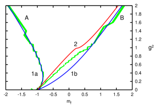
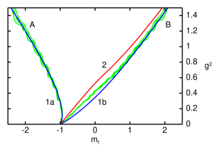
(a) (b)

Figure 6:
(a): A plot of the phase transition lines, A and B, in four dimensions and of the approximations we made. The approximation for the no-loop condensation line, 1a, is very good. For $g^{2}>1$ the same approximation works also very good for the loop condensation line, 1b, while the other approximation, 2, deviates in a qualitatively expected way from the loop condensation line.
(b): A plot of the phase transition lines, A and B, in three dimensions and of the approximations we made. The approximation for the no-flux condensation line, 1a, is very good. For $g^{2}>0.6$ the same approximation works also very good for the flux condensation line, 1b, while the other approximation, 2, deviates in an expected way from the flux condensation line.

In figure 6(a) we have plotted the approximations for the condensation lines in four dimensions and some specific height lines, which characterise the position of the phase transitions. We see that the approximation of the condensation of the no-loops is very good. For $g^{2}>1$ the same method works also very well for the loop condensation line. The other approximation for the loop condensation line does not work as well, but we qualitatively understand why.
The three dimensional case:

In three dimensions we follow the same strategy. We repeat the arguments given for the four dimensional case, leading to exactly the same equations (8) and (10), where we only have to replace the four dimensional quantities by their three dimensional counterparts. In particular $c_{4D}$ is replaced by $c_{3D}$ and $\langle\cos{\tilde{F}}\rangle_{4D}$ is replaced by $\langle\cos{\tilde{F}}\rangle_{3D}$.

In figure 6(b) we plotted the resulting condensation lines for the three dimensional theory. The plot shows some specific height lines which characterise the phase transitions as well as the approximations for the lines where the phase transitions should occur. Again we find that the approximation for the no-flux condensation line is very good. The approximation of the analogue of equation (8) is very good for larger values of $g^{2}$, whereas the deviation of the other approximation to the flux condensation line is qualitatively understood.

4.3 Contours of constant flux density

In this subsection we will approximate the flux density in the region between the two flux condensation lines, by assuming that in this region the correlation lengths of both fields are zero, so that it suffices to look at the single plaquette.

This means that we get the same answer for the three and four dimensional case. The fraction of plaquettes being pierced by an Alice flux, $\rho_{f}$, can be approximated by:

$$\rho_{f}\approx\frac{e^{s_{f}-I_{f}}}{e^{s_{f}-I_{f}}+e^{s_{nf}}\int^{2\pi}_{0}\frac{d\tilde{F}}{2\pi}~{}e^{-I_{\tilde{F}}}}~{}.$$ (11)

Using $s_{f}=s_{nf}$ and $I_{f}=\frac{m_{f}}{g^{2}}$ this gives:

$$m_{f}=g^{2}\ln{\frac{1-\rho_{f}}{\rho_{f}}}-g^{2}\ln{\int^{2\pi}_{0}\frac{d\tilde{F}}{2\pi}~{}e^{-I_{\tilde{F}}}}~{},$$ (12)

which leads to:

$$m_{f}=g^{2}\ln{\frac{1-\rho_{f}}{\rho_{f}}}-g^{2}\ln{I_{0}(\frac{1}{g^{2}})}~{}.$$ (13)

Note that in the limit $g^{2}\to 0$ we find that all the height lines meet at $m_{f}=-1$, just as one should expect, whereas in the $\mathbb{Z}_{2}$ limit one obtains that $\frac{m_{f}}{g^{2}}=\ln{\frac{1-\rho_{f}}{\rho_{f}}}$.

In four dimensions, within the region of the two condensation lines, which is the region we are probing, our approximation works very well, see figure 7(a). In three dimensions the approximation does not work in the whole region, but works very well between the height lines $0.7$ and $0.3$, see figure 7(b).

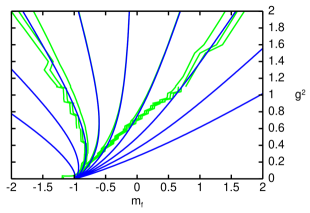
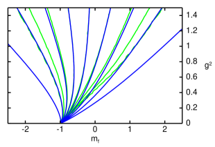
(a) (b)

Figure 7:
(a): Contour lines of the flux density in four dimensions and their approximations. We plotted from, left to right, the height lines: $0.9,0.8,\cdots,0.2,0.1$. The approximations for the height lines $0.6,\cdots,0.4$ are perfect up to the point where they reach the condensation line.
(b): Contour lines of the flux density in three dimensions and their approximations. We plotted from, left to right, the height lines: $0.9,0.8,\cdots,0.2,0.1$. The approximations for the height lines $0.7,\cdots,0.3$ are very good up to the point where they reach the condensation line.

The approximation of the flux density, equation (13), can be split into two parts. The first term on the right hand side is due to the $\mathbb{Z}_{2}$ degrees of freedom. In the $\mathbb{Z}_{2}$ limit this term can be compared with pure $\mathbb{Z}_{2}$ gauge theory, which we did not use as input in this estimate. The second term on the right hand side is due to the $U(1)$ degrees of freedom. Moving away from the $0.5$ height line makes the approximation of $\mathbb{Z}_{2}$ term less good while moving from the $0.9$ height line to the $0.1$ height line makes the $U(1)$ term less good. The validity of the $U(1)$ term can be seen by fitting the $\mathbb{Z}_{2}$ part of the approximation with results from pure $\mathbb{Z}_{2}$ gauge theory. This gives a perfect fit for all values $g^{2}$ for a high flux density, but as one expects, fails in the region of low flux density and small $g^{2}$.

4.4 The monopole/instanton density

In this subsection we will approximate the monopole/instanton density. In the phase where the Alice fluxes do not condense the monopole condensation line and height lines are easily understood. In this phase there are almost no fluxes, and ignoring these the model becomes a pure $U(1)$ theory and on expects the monopole density to behave accordingly, allowing us to use the known numerical results.

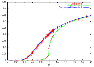
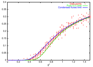
(a) (b)

Figure 8:
(a): A plot of the monopole density. Just as in figure 5(a) all the data points, i.e. including those for different values of $m_{f}$ and $g^{2}$, perfectly match the two different approximations. The monopole density is or equal to the pure $U(1)$ monopole density or is (almost) equal to the approximation for the condensed fluxes phase.
(b): A plot of the instanton density. The instanton density lies between the two different approximations. That the data does not jump from one line to the other line is due to the fact that the $\mathbb{Z}_{2}$ transition is much softer in three dimensions. The points outside the region between the two limits are points where the flux density is very high, implying that the statistics is bad.

In the phase where the Alice fluxes do condense we may approximate the monopole density by the monopole density of a single cube. That this can be done follows basically from the results of sections 4.1 and 4.3. The cubes not pierced by any $\mathbb{Z}_{2}$ flux are in the condensed phase isolated in the sense that the $U(1)$ degrees of freedom of the links have hardly any effect on the surrounding plaquettes. This makes it safe to use the single cube approximation in the phase where the fluxes have condensed.

We determined the single cube density by using random link values, with which we determined the energy of the cube, the charge inside the cube and the entropy of the configuration. With this information we calculated the monopole density for different values of $g^{2}$ and compared it with the data points we found. This approximation is the same for the three and four dimensional model, though in three dimensions these are of course instantons.

Just as in section 4.1 one expects the two approximations to describe the model very well in four dimensions, but in three dimensions one expects an intermediate region. This is exactly what we find, see figures 8(a) and 8(b). Again we note that the points outside the region bounded by the two approximations are points where the flux density is very high, i.e. the fluctuations become very large.

4.5 Discussion

The approximations we made in the last few sections describe the model fairly well. In four dimensions the approximations work extremely well. The phase with condensed fluxes can apparently be understood as a phase where the correlation lengths of the fields are vanishingly small. In three dimensions the division of the phase space is not as clear, but our approximation of the height lines of the flux density does imply a region where the correlation length of both fields is also vanishingly small. If the Alice fluxes do not condense the theory is very well described by a pure compact $U(1)$ gauge theory.

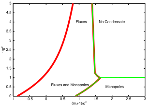
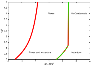
(a) (b)

Figure 9: The phase diagrams of four, (a), and three, (b), dimensional LAED in the new parameters. The details and implications are explained in the text.

As mentioned before, the fact that all the contour lines of the flux density come together at $m_{f}=-1$ for $g^{2}\to 0$, does not mean that the phase transition becomes or stays first order. It is mainly due to the choice of parameters that all the contour lines of the flux density come together. If one uses the in some sense more natural parameters $(m_{f}+1)/g^{2}$ and $1/g^{2}$, it is not at all clear that this will happen. This is illustrated in in figure 9, where we have plotted the phase diagram of the model in terms of the conventional parameters. The crossover transitions are not marked, they are associated to regions with different condensates not separated by a phase transition line. Although there is a second flux transition line, the “no-flux” condensation, there is no monopole/instanton transition at this point. We deduce this from the results of section 4.4. The fact that we are not able to determine the monopole/instanton density there is due to the fact the fluctuations are very large in that region of parameter space. However one would expect the single cube approximation of section 4.4 also to be valid in that region of parameter space.

The position of the monopole transition line, see figure 9(a) is also following from the results of section 4.4. We pointed out that the monopole data splits up into two regions, the regions where the fluxes have or have not condensed. This means that the $U(1)$ monopole transition line splits up and follows the (first) flux transition line. We have drawn it all the way along this flux condensation line, but it is not yet clear whether there is always a monopole transition. For $g^{2}\to 0$ and $g^{2}\to\infty$ the difference in the monopole density between the two regions becomes smaller and smaller.

To some extend the same is true for the instanton density, see figure 9(b). Although in that case there is an intermediate region, see section 4.4. In this region the instanton density grows with increasing flux density, and since in this region the flux density has a transition one would expect also the instanton density to show a transition. The data also appears to imply this, but is not shown here. Again it is not clear what happens to this transition in the limits of $g^{2}\to 0$ and $g^{2}\to\infty$. In these limits the difference of the instanton density between the regions where the fluxes have or have not condensed goes to zero.

5 Conclusions and outlook

We have studied Alice electrodynamics on a lattice, with a model that allows the formation of magnetic monopoles and Alice fluxes. It includes the usual Wilson lattice action for the $U(1)$ gauge theory and has an extra bare mass term for Alice fluxes. This term suffices to reach all four phases of Alice electrodynamics given in table 1.

We have determined the regions in phase space corresponding to the four different phases of LAED and presented results on some measurable quantities; the monopole density, the flux density and $\langle\cos{\tilde{F}}\rangle$. We then approximated the locations of the flux and the so called no-flux condensation line in the phase diagram of the model, both in three and four dimensions. These approximations worked very well except for the flux condensation line for small values of the gauge coupling. The other approximations we made also all work quite well, with the remark that in three dimensions there is an intermediate region which we have not yet investigated. We successfully compared our numerical results with approximations of the flux density between the flux and the no-flux condensation line, the monopole/instanton density, $\langle\cos{\tilde{F}}\rangle$ and the position of the monopole condensation line. The monopole condensation becomes a crossover in the region where the Alice fluxes are condensed. In section 4.5 we gave the resulting phase diagrams.

It would be interesting to examine the fate of the phase transitions in the monopole and instanton density induced by (first) condensing Alice fluxes for small and large values of $g^{2}$. For small values of $g^{2}$ it is also not clear if the two flux transitions merge or not in the parameter space with the coordinates $(m_{f}+1)/g^{2}$ and $1/g^{2}$. In a forthcoming paper we will address interesting questions concerning the screening versus confinement of charges and/or magnetic monopoles in the various phases of the theory.

We thank Jan Smit and Jeroen Vink for valuable advice and support related to lattice gauge theories. This work was partially supported by the ESF COSLAB program.

References

- [1] A. S. Schwarz, Field theories with no local conservation of the electric charge, Nucl. Phys. B 208 (1982) 141.
- [2] Mark Alford, Katherine Benson, Sidney Coleman, John March-Russell, and Frank Wilczek, Zero modes of nonabelian vortices, Nucl. Phys. B 349 (1991) 414–438.
- [3] Kenneth G. Wilson, Confinement of quarks, Phys. Rev. D 10 (1974) 2445–2459.
- [4] F. A. Bais and J. Striet, On a core instability of ’t Hooft Polyakov type monopoles, Phys. Lett. B 540 (2002) 319–323.
- [5] C. B. Lang and T. Neuhaus, Compact U(1) gauge theory on lattices with trivial homotopy group, Nucl. Phys. B 431 (1994) 119–130.
- [6] R. Balian, J. M. Drouffe, and C. Itzykson, Gauge fields on a lattice 2. Strong coupling expansions and transition points, Phys. Rev. D 11 (1975) 2104.
- [7] Gyan Bhanot and Michael Creutz, The phase diagram of Z(n) and U(1) gauge theories in three- dimensions, Phys. Rev. D 21 (1980) 2892.
- [8] Michael Creutz, Laurence Jacobs, and Claudio Rebbi, Monte Carlo study of abelian lattice gauge theories, Phys. Rev. D 20 (1979) 1915.
- [9] T. A. DeGrand and Doug Toussaint, Topological excitations and Monte Carlo simulation of abelian gauge theory, Phys. Rev. D 22 (1980) 2478.
- [10] Burkard Klaus and Claude Roiesnel, High-statistics finite size scaling analysis of U(1) lattice gauge theory with a Wilson action, Phys.Rev. D 58 (1998) 114509.