Calorons, instantons and constituent monopoles in SU(3) lattice gauge theory

Abstract

We analyze the zero-modes of the Dirac operator in quenched SU(3) gauge configurations at non-zero temperature and compare periodic and anti-periodic temporal boundary conditions for the fermions. It is demonstrated that for the different boundary conditions often the modes are localized at different space-time points and have different sizes. Our observations are consistent with patterns expected for Kraan - van Baal solutions of the classical Yang-Mills equations. These solutions consist of constituent monopoles and the zero-modes are localized on different constituents for different boundary conditions. Our findings indicate that the excitations of the QCD vacuum are more structured than simple instanton-like lumps.

Understanding the relevant excitations of the QCD vacuum is a major scientific goal and lattice calculations can contribute valuable non-perturbative information. A prominent candidate for such relevant excitations are instantons which are particularly successful in providing a mechanism for chiral symmetry breaking [1]. Lattice calculations have helped to corroborate these ideas. Recently several studies of the zero-modes and near zero-modes of the Dirac operator [2, 3, 4] which provide a powerful and natural filter retaining the infrared fluctuations of the underlying gauge field were presented. It was established that the vacuum has a lumpy structure and the lumps are locally chiral [3] and (anti) self-dual [4].

However, it is generally believed, that instantons are not responsible for confinement. On the other hand all lattice calculations show that the deconfinement transition and the restoration of chiral symmetry coincide at a single critical temperature which suggests that there is an underlying mechanism linking the two phenomena. In recent years Kraan and van Baal [5] have constructed new solutions for the classical SU(N) Yang Mills equations with compactified time, i.e. at finite temperature (KvB solutions). The KvB solutions generalize the caloron solution [6] and a lump of topological charge $1$ is built of N constituent monopoles, a feature which might provide a link to the confinement problem. Note that for KvB solutions the monopole lumps appear in multiples of N. A single lump is not an independent object and only N lumps together have topological charge $\pm 1$. Strong evidence for SU(2) KvB solutions in cooled lattice gauge configurations were given for twisted [7] and periodic boundary conditions [8]. The zero-mode for the KvB solution [9] shows characteristic features which should allow to use the eigenvectors of the Dirac operator as a filter retaining infrared fluctuations and search for traces of KvB solutions also in thermalized configurations.

Before presenting our lattice calculations we briefly discuss a few properties of SU(3) KvB solutions and their zero-mode. KvB solutions [5] are characterized by the Polyakov loop at spatial infinity which in a suitable gauge can be expressed as $P_{\infty}=\exp(i2\pi\mbox{diag}(\mu_{1},\mu_{2},\mu_{3}))$ with $\mu_{1}+\mu_{2}+\mu_{3}=0$ and $\mu_{1}\leq\mu_{2}\leq\mu_{3}\leq\mu_{4}\equiv 1+\mu_{1}$. The action density can be written down in a relatively simple form [5] and depends in addition to the phases $\mu_{1},\mu_{2},\mu_{3}$ also on three 3-vectors $\vec{y}_{1},\vec{y}_{2},\vec{y}_{3}$. As remarked the KvB solutions can be seen to be superpositions of constituent monopoles and the 3 corresponding lumps are in space located at $\vec{y}_{1},\vec{y}_{2},\vec{y}_{3}$. The $m$-th constituent monopole can be assigned a mass $8\pi^{2}(\mu_{m+1}-\mu_{m})$ (both the masses and the monopole positions $\vec{y}_{i}$ are in units of the inverse temperature). A general choice for the parameters of the KvB solution will give rise to three lumps at different positions with different width.

The zero-mode $\psi$ in the background of a KvB solution has been computed [9] for arbitrary temporal boundary conditions $\psi(t+1/T,\vec{x})=\exp(i2\pi z)\psi(t,\vec{x})$ with $z=1/2$ corresponding to anti-periodic boundary conditions (b.c.) and $z=0$ giving the periodic case. The remarkable feature of the zero-mode is that it traces only one of the monopoles. In particular it is located on the $m$-th monopole when $z\in\{\mu_{m},\mu_{m+1}\}$. At least for well separated monopoles the width of the lump seen by the zero-mode depends on the size of the underlying gluonic lump and also the quantity $\sigma=\min[z-\mu_{m},\mu_{m+1}-z]$. The lump is narrow for large $\sigma$ and broad for small $\sigma$. This is an important feature in the deconfined phase where due to the $Z_{3}$ symmetry of the action the Polyakov loop can have three different phases $0,\pm 2\pi/3$. At sufficiently high temperatures configurations with real Polyakov loop have $\mu_{i}\sim 0,i=1,2,3$. The anti-periodic zero-mode has $z=1/2$, is located on monopole 3 and has $\sigma\sim 1/2$ and thus is quite localized. The periodic zero-mode with $z=0$ can be located on any of the monopoles. It has $\sigma\sim 0$ and is very broad. For configurations with phase $2\pi/3$ of the Polyakov loop (the case with phase $-2\pi/3$ is similar) one has $(\mu_{1},\mu_{2},\mu_{3})\sim(-2/3,1/3,1/3)$. The anti-periodic mode has $\sigma\sim 1/6$ while the periodic mode has $\sigma\sim 1/3$ and both of them are localized on monopole 1. This implies that for complex Polyakov loop the roles are reversed and here the periodic mode is more localized. However, the difference in localization is not as pronounced since the values $\sigma\sim 1/6$ and 1/3 differ less than $\sigma\sim 1/2$ and 0 obtained for real Polyakov loop.

To summarize, if KvB solutions are present in thermalized SU(3) gauge configurations then one should find instances where the zero-modes with anti-periodic b.c. and periodic b.c. are located at different positions and the lumps they see can differ in size. In the deconfined phase the differences in size should show a particular pattern when comparing configurations with real and complex Polyakov loop. These are simple stable signatures which distinguish KvB solutions from instantons or calorons.

In our numerical analysis we use quenched SU(3) gauge configurations generated with the Lüscher-Weisz action [10] on $6\times 20^{3}$ lattices. We adjust the inverse gauge coupling $\beta$ such that one ensemble is below the critical temperature and the other one in the deconfined high temperature phase. The lattice spacing $a$ and the values for the temperature $T$ and $T_{c}$ for the Lüscher-Weisz action listed in Table I were determined in [11].

size	$\beta$	statistics	$a$ [fm]	$T$ [MeV]	$T/T_{c}$
$6\times 20^{3}$	8.20	70	0.115	287	0.96
$6\times 20^{3}$	8.45	64 + 25	0.094	350	1.17

TABLE I.: Parameters of our calculations.

We calculate the eigenvalues and eigenvectors of the chirally improved Dirac operator [12] using the implicitly restarted Arnoldi method [13]. This is done for both, periodic and anti-periodic temporal b.c. for the fermions (the spatial b.c. are always periodic). The chirally improved Dirac operator is not exactly chiral but a good approximation of an exactly chiral lattice Dirac operator. The topological zero-modes of the continuum manifest themselves as small real modes. It can be shown [14] that although the eigenvalues are not exactly zero they give rise to the correct topological susceptibility through the index theorem. Although the small real eigenvalues do not vanish exactly we will refer to the corresponding modes as zero-modes in the following. From a larger set of configurations we select those configurations which have a single zero-mode for both b.c., i.e. are in the sector with topological charge $Q=\pm 1$. The restriction to the $|Q|=1$ sector is necessary to avoid mixing between multiple zero-modes that occurs in higher sectors. For our configurations with $|Q|=1$ we find that for both, periodic and anti-periodic boundary conditions the zero-mode is always dominated by a single lump. The position of the lump, however, can be different for the two choices of the boundary conditions.

The ensemble in the high temperature phase has a non-vanishing Polyakov loop. We will use this ensemble to study the influence of the expectation value of the Polyakov loop on the zero-modes. We divide the deconfining ensemble into sub-ensembles with complex respectively real Polyakov loop containing 64 (25) configurations. We will refer to these subensembles as the complex respectively the real sector.

In order to analyze the localization of the zero modes we form the scalar density $\rho(x)=\sum_{c,d}|\psi(x)_{c,d}|^{2}$ from the zero-modes $\psi(x)_{c,d}$ by summing over the color and Dirac indices $c,d$. The resulting density $\rho$ is gauge invariant. In Fig. 1 we show $y$-$z$ slices of the scalar density and compare the anti-periodic case (l.h.s.) to the periodic case (r.h.s.). The plots are for a configuration in the confining phase.

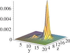
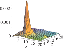
FIG. 1.: Scalar density of the zero-mode for anti-periodic temporal b.c. (l.h.s.) and periodic temporal b.c. (r.h.s.). We show $y$-$z$ slices for a configuration below $T_{c}$.

Fig. 1 clearly demonstrates that the zero-modes with periodic and anti-periodic b.c. are located at different space-time points. For anti-periodic b.c. $\rho$ has its maximum at $(t,x,y,z)=(2,9,13,13)$ while for periodic b.c. it is located at (1,9,6,7). The figure shows the $y$-$z$ slices through the maxima, i.e. the $t=2,x=9$ slice for anti-periodic b.c., respectively the $t=1,x=9$ slice for the periodic case. The maxima are separated by 9.3 lattice spacings which corresponds to 1.1 fm. It is also obvious from the figure that the two lumps have different height and width. This is not what is expected for the zero-mode of a classical caloron but agrees well with the behavior predicted for the KvB solutions. When scanning through our ensemble we have detected many configurations showing such behavior.

Having found instances of configurations resembling KvB solutions we now turn to a more quantitative analysis. One interesting observable was already addressed, the distance between the maximum of $\rho_{A}$ and the maximum of $\rho_{P}$. The subscript $A$ refers to $\rho$ computed from the zero mode with anti-periodic b.c, while the subscript $P$ is used for $\rho$ computed from the periodic zero-mode.

A related observable is the overlap of the support of the two lumps. The support is defined as the function $\theta(x)$ which has $\theta(x)=1$ for the lattice points $x$ carrying the lump in $\rho$ and $\theta(x)=0$ for all other points. An open question is how to identify the lump. For a narrow lump the support is small while a broad lump has a much larger support.

We will base our definition of the support on the so-called inverse participation ratio $I=V\sum_{x}\rho(x)^{2}$, where $V$ is the total number of points in our lattice. Note that we use normalized eigenvectors such that $\sum_{x}\rho(x)=1$. It is easy to see that for an entirely localized state ($\rho(x)=1$ for only one lattice point and 0 else) the inverse participation ratio is $I=V$, while for a completely delocalized state ($\rho(x)=1/V$ for all lattice points) $I=1$. The inverse participation ratio is a convenient measure for the localization, assuming large values for localized states and small values for spread out states.

Using $I$ we now define a number $N=V/(32I)$ and use this to determine the support by setting $\theta(x)=1$ for those $N$ lattice points $x$ which carry the $N$ largest values of $\rho$ and $\theta(x)=0$ for all other points. The normalization of $N$ was chosen such that if the lump was a 4-D Gaussian the support would consist of the 4-volume carrying the points inside the half-width of the Gaussian. Note that $N$ is the size of the support, i.e. $N=\sum_{x}\theta(x)$.

With our definition of the support $\theta$ for both the anti-periodic ($\theta_{A}$) and periodic ($\theta_{P}$) lumps we can define the overlap function $C$ of the two lumps as $C(x)=\theta_{P}(x)\theta_{A}(x)$. From this we compute the relative overlap $R=2/(N_{A}+N_{P})\sum_{x}C(x)$. The relative overlap $R$ is a real number ranging from 0.0 to 1.0. If the lump in $\rho_{A}$ and the lump in $\rho_{P}$ sit on top of each other (at least the core up to about the half-width) and have the same size then $R=1.0$. If the two lumps are entirely separated one has $R=0.0$. Values in between give the ratio of the common volume of the two supports to the average size of the two supports. Note that even if the two lumps sit on top of each other, but have different sizes $N_{A},N_{P}$ one has $R<1.0$.

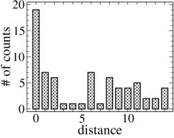
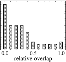
FIG. 2.: Histograms for the distance of the maxima (l.h.s.) and the relative overlap of the lumps for different boundary conditions (r.h.s.). The data are for the ensemble below $T_{c}$.

In Fig. 2 we show histograms for the distance between the maxima in $\rho_{A}$ and $\rho_{P}$ (l.h.s.) and histograms for the relative overlap (r.h.s). The distances were rounded to the nearest integer while the relative overlap $R$ was rounded to the nearest multiple of $0.1$. The data shown are for the ensemble below $T_{c}$. When looking at the l.h.s. plot one finds that for many configurations the maxima of the two lumps sit on top of each other. However, the distribution shows also that for 50% of the configurations the two lumps are separated by at least 6 lattice spacings which corresponds to 0.7 fm, almost twice the typical instanton size. This indicates that for a large fraction of the ensemble the zero-modes with different b.c. see different lumps.

Also from the histograms for the relative overlap (r.h.s. plot in Fig. 2) one comes to the same conclusion. Only for a small fraction of the configurations one finds that the lumps seen by anti-periodic and periodic zero-modes coincide and for many cases they do not overlap at all. A comparison of the two plots in Fig. 2 shows that although many pairs of lumps may have the same position of their maximum they still differ in size such that their relative overlap is smaller than 1.

In order to further study the evidence for KvB solutions we now turn to the ensemble in the high-temperature phase. For these configurations the theory is deconfined and the Polyakov loop has a non-vanishing expectation value. As discussed above the phase of the Polyakov loop plays an important role for the properties of the KvB solutions and one expects significant differences between the complex and the real sector.

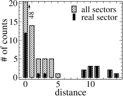
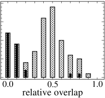
FIG. 3.: Same as Fig. 2 but for the ensemble above $T_{c}$.

Let us begin our discussion of the deconfined phase by again looking at the histograms for the distance between the peaks of $\rho$ and their overlap. Fig. 3 is equivalent to Fig. 2 but now shows data for the ensemble above $T_{c}$. In addition to showing the data for the full ensemble we also display the results for the subensemble in the real sector. These data are represented by thinner, black bars.

When inspecting the histograms for the distance between the peaks (l.h.s. plot) we find that again a certain amount of configurations shows rather large distances but the fraction of these configurations is smaller. 12% of the ensemble show distances of at least 7 lattice spacings (again corresponding to $\sim 0.7$ fm). Note that these configurations are entirely dominated by the real sector. This is exactly as pointed out in our summary of the KvB zero-modes where we discussed that in the complex sector the two zero-modes sit on the same lump.

Another effect is evident from the two plots in Fig. 3. Although more than half of the configurations have the center of the two lumps at exactly the same lattice point we do not see many configurations where the lumps have a large overlap. The distribution is instead peaked at an overlap of 0.5. The reason for this behavior is the difference in size between the two lumps. One of them is much narrower than the other one and thus their relative overlap is considerably smaller than 1.

We directly study the phenomenon of the large difference of the sizes of the two lumps by comparing the inverse participation ratio $I$ of the zero-mode for anti-periodic and periodic b.c. ($I_{A},I_{P}$). Fig. 4 shows a scatter plot of our results with the data in the real sector represented by filled circles and open triangles are used for the complex sector. In the real sector one finds that the anti-periodic inverse participation ratio (ranging from $I_{A}\sim 25$ up to $I_{A}\sim 180$) is much larger than its periodic counterpart ($I_{P}\sim$ 2-5). For the complex sector the situation is similar but the role of the boundary conditions is reversed. However, the effect is not as dramatic as in the real sector. For not too localized modes ($I_{P}$ up to 70) one finds that the inverse participation ratio for the periodic b.c. is about 3-times larger than for the anti-periodic case. The qualitative pattern for the different sectors of the Polyakov loop matches the predictions for KvB solutions discussed in our summary of the properties of the KvB zero-modes.

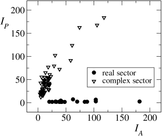
FIG. 4.: Comparison of the inverse participation ratio of the zero mode for periodic ($I_{P}$) and anti-periodic ($I_{A}$) b.c. The data are from the ensemble above $T_{c}$.

We remark that we have performed an equivalent analysis also on a $16^{4}$ lattice at $a=0.094$ fm. Although this is a typical lattice for zero-temperature calculations we still find a substantial amount of configurations with zero-modes showing the characteristic properties of KvB solutions. This observation might account for the failure of identifying the profile of classical instanton zero-modes in quenched lattice configurations [15].

In this letter we have studied zero-modes of the Dirac operator for gauge configurations with topological charge $\pm 1$ for temperatures slightly below $T_{c}$ and a second ensemble in the deconfined phase above $T_{c}$. Analyzing the localization of the zero-modes we observed large differences when comparing temporal anti-periodic and periodic b.c. for the fermions. For a substantial portion of the ensemble we found that the zero-mode is located at different positions for different b.c. and also the width of the lumps can differ substantially. For the ensemble in the deconfined phase we observed that the behavior also depends on the phase of the Polyakov loop. The emerging picture for the zero-modes is qualitatively well described by the properties of the zero-modes of Kraan - van Baal solutions. Our results indicate that the picture of topological excitations being single lumps might be too simple and a substructure resembling the constituent monopoles of Kraan - van Baal solutions is evident.

Acknowldegements: I would like to thank Meinulf Göckeler, Michael Müller-Preussker, Paul Rakow, Stefan Schaefer, Andreas Schäfer, Christian Weiss and in particular Pierre van Baal for discussions and the Austrian Academy of Science for support (APART 654). The calculations were done on the Hitachi SR8000 at the Leibniz Rechenzentrum in Munich and I thank the LRZ staff for training and support.

REFERENCES

- [1] D. Diakonov and V.Y. Petrov, Phys. Lett. B 147 (1984) 351; Nucl. Phys. B 272 (1986) 457; T. Schäfer and E.V. Shuryak, Rev. Mod. Phys. 70 (1998) 323 and references therein.
- [2] T.L. Ivanenko and J.W. Negele, Nucl. Phys. Proc. Suppl. 63 (1998) 504; T. DeGrand and A. Hasenfratz, Phys. Rev. D 64 (2001) 034512; M. Göckeler, P.E.L. Rakow, A. Schäfer, W. Söldner, T. Wettig, Phys. Rev. Lett. 87 (2001) 042001; T. DeGrand, Phys. Rev. D 64 (2001) 094508; C. Gattringer, M. Göckeler, C.B. Lang, P.E.L. Rakow, A. Schäfer, Phys. Lett. B 522 (2001) 194; I. Horváth et al., hep-lat/0203027.
- [3] I. Horváth, N. Isgur, J. McCune and H.B. Thacker, Phys. Rev. D 65 (2002) 014502; T. DeGrand and A. Hasenfratz, Phys. Rev. D 65 (2002) 014503; T. Blum et al., Phys. Rev. D 65 (2002) 014504; R.G. Edwards and U.M. Heller, Phys. Rev. D 65 (2002) 014505; I. Hip, T. Lippert, H. Neff, K. Schilling and W. Schroers, Phys. Rev. D 65 (2002) 014506; C. Gattringer, M. Göckeler, P.E.L. Rakow, S. Schaefer, A. Schäfer, Nucl. Phys. B 617 (2001) 101, Nucl. Phys. B 618 (2001) 205; P. Hasenfratz, S. Hauswirth, K. Holland, T. Jörg and F. Niedermayer, Nucl. Phys. Proc. Suppl. 106 (2002) 751.
- [4] C. Gattringer, Phys. Rev. Lett. 88 (2002) 221601.
- [5] T.C. Kraan and P. van Baal, Phys. Lett. B 428 (1998) 268, Nucl. Phys. B 533 (1998) 627, Phys. Lett. B 435 (1998) 389.
- [6] B.J. Harrington and H.K. Shepard, Phys. Rev. D 17 (1978) 2122, Phys. Rev. D 18 (1978) 2990.
- [7] M. Garcia Perez, A. Gonzalez-Arroyo, A. Montero and P. van Baal, JHEP 9906 (1999) 001.
- [8] E.M. Ilgenfritz, B.V. Martemyanov, M. Müller-Preussker, S. Shcheredin and A.I. Veselov, Phys. Rev. D 66 (2002) 074503, hep-lat/0209081.
- [9] M. Garcia Perez, A. Gonzalez-Arroyo, C. Pena and P. van Baal, Phys. Rev. D 60 (1999) 031901; M.N. Chernodub, T.C. Kraan and P. van Baal, Nucl. Phys. Proc. Suppl. 83 (2000) 556.
- [10] M. Lüscher and P. Weisz, Commun. Math. Phys. 97 (1985) 59, Err.: 98 (1985) 433; G. Curci, P. Menotti and G. Paffuti, Phys. Lett. B 130 (1983) 205, Err.: B 135 (1984) 516.
- [11] C. Gattringer, R. Hoffmann and S. Schaefer, Phys. Rev. D 65 (2002) 094503, C. Gattringer, P.E.L. Rakow, A. Schäfer and W. Söldner, Phys. Rev. D 66 (2002) 054502.
- [12] C. Gattringer, Phys. Rev. D 63 (2001) 114501; C. Gattringer, I. Hip, C.B. Lang, Nucl. Phys. B597 (2001) 451.
- [13] D.C. Sorensen, SIAM J.Matrix Anal.Appl.13 (1992) 357.
- [14] C. Gattringer, R. Hoffmann and S. Schaefer, Phys. Lett. B 535 (2002) 358.
- [15] I. Horváth et al., Phys. Rev. D 66 (2002) 034501.