DESY 02-148
Edinburgh 2002/08
LU-ITP 2002/017
September 2002
A non-perturbative determination of $Z_{V}$ and $b_{V}$ for $O(a)$ improved quenched and unquenched Wilson fermions

Abstract

By considering the local vector current between nucleon states and imposing charge conservation we determine, for $O(a)$ improved Wilson fermions, its renormalisation constant and quark mass improvement coefficient. The computation is performed for both quenched and two flavour unquenched fermions.

1 INTRODUCTION

Due to the presence of the ‘Wilson term’ in the lattice fermion action for Wilson fermions the discretisation errors are $O(a)$. As the gluon part of the action (sum of plaquettes) has only $O(a^{2})$ errors, it is also desirable to achieve this for the fermion action. The Symanzik programme allows a systematic reduction of errors to $O(a^{2})$ upon including additional higher dimensional operators. The (on-shell) action is improved with a suitably tuned ‘clover’ term. However it is also necessary to improve each operator separately. Much work has been devoted to this topic in recent years; here we shall just concentrate on the local vector current: $V^{(q)}_{\mu}=\overline{q}\gamma_{\mu}q$. In this case just two additional operators $am_{q}V^{(q)}_{\mu}$ and $\mbox{\small$\frac{1}{2}$}ia\partial_{\lambda}T^{(q)}_{\mu\lambda}$ are required giving the $O(a)$ improved and renormalised vector current as

$${\cal V}_{\mu}^{(q)R}=Z_{V}(1+am_{q}b_{V})(V^{(q)}_{\mu}+\mbox{\small$\frac{1}{2}$}iac_{V}\partial_{\nu}T^{(q)}_{\mu\nu})$$

with $T^{(q)}_{\mu\nu}=\overline{q}\sigma_{\mu\nu}q$. The second improvement operator only has an effect in non-forward matrix elements and will not be considered further here. The renormalisation constant $Z_{V}$ and improvement coefficient $b_{V}$ are functions of the coupling constant $g_{0}$ and perturbatively we have, [2], to one loop (independently of the presence of fermions),

$$Z_{V}(g_{0}) = 1-0.12943g_{0}^{2}+\ldots,$$

$$b_{V}(g_{0}) = 1+0.15323g_{0}^{2}+\ldots,$$

but in presently accessible regions of $\beta\equiv 6/g_{0}^{2}$ there may be considerable deviations.

2 THE CONSERVED CURRENT

There is an exact symmetry of the action $q\to e^{-i\alpha}q$, $\overline{q}\to e^{i\alpha}\overline{q}$ giving via the Noether theorem the Ward identity (WI)

$$\langle\Omega\overline{\Delta}_{\mu}J^{(q)}_{\mu}\rangle=\left\langle{\partial\Omega\over\partial q}q\right\rangle+\left\langle\overline{q}{\partial\Omega\over\partial\overline{q}}\right\rangle,$$

where $\Omega$ is an arbitrary operator, $\overline{\Delta}_{\mu}$ is the lattice backward derivative, and $J^{(q)}_{\mu}$ the exactly conserved vector current ($CVC$),

$$J^{(q)}_{\mu}(x+\mbox{\small$\frac{1}{2}$}\hat{\mu})=$$

$$\mbox{\small$\frac{1}{2}$}\left[\overline{q}_{x}(\gamma_{\mu}-1)U_{\mu}(x)q_{x+\hat{\mu}}-\overline{q}_{x+\hat{\mu}}(\gamma_{\mu}+1)U_{\mu}(x)^{\dagger}q_{x}\right]$$

Roughly speaking the RHS of this equation counts the number of $q$ and $\overline{q}$ in operator $\Omega$. For our numerical results we take $\Omega\to B\overline{B}$ where $B$ is the (unpolarised) nucleon operator to give, upon solving the WI equation,

$$R(J^{(u-d)}_{4}) = {\langle B(t)J^{(u-d)}_{4}(\tau)\overline{B}(0)\rangle\over\langle B(t)\overline{B}(0)\rangle}$$ (3)

$$= \left\{\begin{array}[]{ll}c_{1}^{(u-d)}&0<\tau<t\\ c_{2}^{(u-d)}&t<\tau<N_{T}-1\end{array}\right.$$

($J_{4}^{(u-d)}\equiv J_{4}^{(u)}-J_{4}^{(d)}$) where $c_{i}^{(u-d)}$ are constants and with jump, $\Delta R(J_{4}^{(u-d)})\equiv c_{1}^{(u-d)}-c_{2}^{(u-d)}=1$, ie charge conservation. The numerical advantage of considering $u-d$ is that the hard to compute quark line disconnected terms cancel. (For the $CVC$ this term vanishes though.) In Fig. 1 we show this ratio for the conserved vector current.

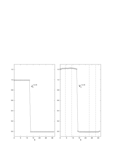
Figure 1: $R(J_{4}^{(u-d)})$ and $R(V_{4}^{(u-d)})$ plotted against the operator position $\tau$ for the quenched ($n_{f}=0$) data set $\beta=6.0$, $\kappa=0.1342$ on a $N_{S}^{3}\times N_{T}=16^{3}\times 32$ lattice with $t=13$. Typical fit intervals for $V_{4}^{(u-d)}$ are given by the pairs of vertically dashed lines.

A very good signal is observed (indeed the result should be true to machine accuracy).

3 THE LOCAL CURRENT

The local vector current ($LVC$) is not conserved on the lattice and so we do not expect the jump to be equal to one. This is shown in the RH picture in Fig. 1. We now define the renormalisation constants ($Z_{V}$, $b_{V}$) by demanding that the renormalised local current has the same behaviour as the conserved current, so that

$$Z_{V}(1+am_{q}b_{V})=\left[\Delta R(V_{4}^{(u-d)})\right]^{-1}.$$

Thus upon plotting the data, the intercept gives $Z_{V}$ and the gradient $Z_{V}b_{V}$. ($am_{q}=\mbox{\small$\frac{1}{2}$}(1/\kappa-1/\kappa_{c})$ and $\kappa_{c}(g_{0})$ is estimated from $r_{0}m_{q}\propto(r_{0}m_{ps})^{2}$.) In Fig. 2 we show quenched results from which the intercept and gradient can be found.

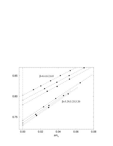
Figure 2: $\Delta R(V_{4}^{(u-d)})$ for quenched configurations for $\beta=6.4$, $6.2$ and $6.0$ (upper set of curves, top to bottom respectively) and for the unquenched configurations for $\beta=5.29$, $5.25$ and $5.20$ (lower set of curves).

Other alternative non-perturbative determinations have been given by the ALPHA collaboration, [3], using the Schrödinger functional, the LANL collaboration, [4] using other Ward identities and Martinelli et al., [5] by ‘mimicking’ perturbation theory.

As well as quenched data sets ($n_{f}=0$), in collaboration with UKQCD, we have also generated unquenched data sets. In this study we use the configurations with parameters given in Table 1.

$\beta$	$\kappa_{sea}$	Volume	Trajs.	Group
5.20	0.1342	$16^{3}\times 32$	5000	QCDSF
5.20	0.1350	$16^{3}\times 32$	8000	UKQCD
5.20	0.1355	$16^{3}\times 32$	8000	UKQCD
5.25	0.1346	$16^{3}\times 32$	2000	QCDSF
5.25	0.1352	$16^{3}\times 32$	8000	UKQCD
5.25	0.13575	$24^{3}\times 48$	1000	QCDSF
5.29	0.1340	$16^{3}\times 32$	4000	UKQCD
5.29	0.1350	$16^{3}\times 32$	5000	QCDSF
5.29	0.1355	$24^{3}\times 48$	2000	QCDSF

Table 1: Data sets used in the unquenched, $n_{f}=2$, simulations.

We now present our results. In Fig. 3

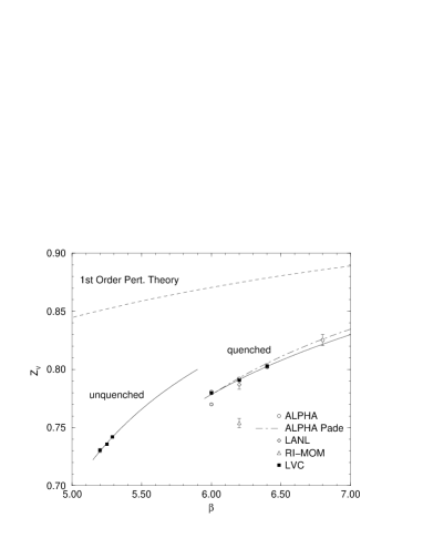
Figure 3: $Z_{V}$ ($LVC$, filled squares) determined in this work for quenched and unquenched $O(a)$ improved fermions. For the quenched case a comparison is made with ALPHA, [3], LANL, [4] and RI-MOM, [5]. Padé fits are also given for our and the ALPHA results.

we show $Z_{V}$ and in Fig. 4,

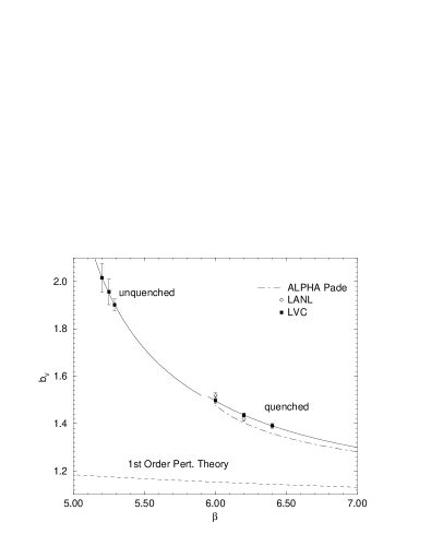
Figure 4: $b_{V}$ ($LVC$, filled squares) determined in this work again for both quenched and unquenched $O(a)$ improved fermions. Also shown is the Padè fit from ALPHA, [3], and the LANL, [4] results for quenched fermions.

$b_{V}$. For quenched fermions good agreement with other methods is found.

4 CONCLUSIONS

The method described here reproduces the results of other approaches for $O(a)$ improved quenched fermions. (But one needs to remember that $Z_{V}$ definitions can vary by $O(a^{2})$ while $b_{V}$ definitions may vary by $O(a)$.) For $O(a)$ improved unquenched fermions $Z_{V}$ is smaller and $b_{V}$ larger than for quenched fermions at the same lattice spacing (roughly $a_{n_{f}=2}(5.25)\sim a_{n_{f}=0}(6.0)$). Further details and final results will appear in [6].

References

[1]
M. Lüscher, hep-lat/9802029.
[2]
E. Gabrielli et al.,
Nucl. Phys. B362 (1991) 475;
M. Göckeler et al.,
Nucl. Phys. Proc. Suppl. 53 (1997) 896, hep-lat/9608033;
S. Sint et al.,
Nucl. Phys. B502 (1997) 251, hep-lat/9704001.
[3]
M. Lüscher et al.,
Nucl. Phys. B491 (1997) 344, hep-lat/9611015.
[4]
T. Bhattacharya et al.,
Nucl. Phys. Proc. Suppl. 106 (2002) 789, hep-lat/0111001.
[5]
G. Martinelli at al.,
Nucl. Phys. B445 (1995) 81, hep-lat/9411010;
D. Becirevic et al.,
Nucl. Phys. Proc. Suppl. 83 (2000) 863, hep-lat/9909039.