Finite density QCD via imaginary chemical potential

Abstract

We study QCD at nonzero temperature and baryon density in the framework of the analytic continuation from imaginary chemical potential. We carry out simulations of QCD with four flavor of staggered fermions, and reconstruct the phase diagram in the temperature–imaginary $\mu$ plane. We consider ansätze for the analytic continuation of the critical line and other observables motivated both by theoretical considerations and mean field calculations in four fermion models and random matrix theory. We determine the critical line, and the analytic continuation of the chiral condensate, up to $\mu_{B}\simeq 500$ MeV. The results are in qualitative agreement with the predictions of model field theories, and consistent with a first order chiral transition. The correlation between the chiral transition and the deconfinement transition observed at $\mu=0$ persists at nonzero density.

I Introduction

QCD at finite temperature and density is of fundamental importance, both on purely theoretical and phenomenological grounds. At high temperature asymptotic freedom will produce deconfinement and chiral symmetry restoration, at high density a richer phase structure and new phenomena have been predicted [1]. In principle, the lattice formulation provides a rigorous framework for the study of such phenomena. In practice, however, the lattice regularization is usually combined with importance sampling, which cannot be naively applied at nonzero baryon density, where the quark determinant becomes complex [2].

It has been recently realized [3] that this problem can be circumvented in the high $T$, low $\mu$ part of the QCD phase diagram where one can take advantage of physical fluctuations [4] Interesting physical information can be obtained by computing the derivatives with respect to $\mu$ at zero chemical potential and high temperature [5, 6, 7]. Fodor and Katz proposed an improved reweighting and applied it to the study of the four [8] and two plus one flavor model [9] . In refs. [10, 11, 12] the imaginary chemical potential approach was advocated and exploited in connection with the canonical formalism. In ref. [13] it was proposed that the analytic continuation from imaginary chemical potential could be practical at high temperature, and the idea was tested in the infinite coupling limit. In refs. [14]  [15] the method was applied successfully to the dimensionally reduced model. In ref. [16] it was proposed that the critical line itself can be analytically continued and results for two flavor of staggered fermions were presented.

In this work we study QCD with four flavors of staggered fermions within the imaginary chemical potential approach. Some of the results presented here have been preliminarly reported in [17]

In the next Section we review the formalism and the method. In Section III we reconstruct the phase diagram in the temperature–imaginary chemical potential plane. This is an interesting physical question by itself, it is a mandatory step toward the reconstruction of the phase diagram for real chemical potential, and provides some guidance for the analytic continuation. In Section IV we discuss a few aspects of the analytic continuation and offer two examples from model field theories: we will note there that by considering $\mu^{2}$ rather than $\mu$, an analogy can be made between QCD at finite baryon density and ordinary statistical systems in external fields. The remaining part of the paper is devoted to numerical results at nonzero baryon density. The critical line is presented Section V, including a first assessment of the dependence on the number of flavors obtained combining the results by de Forcrand and Philipsen [16] with ours, and a cross check with the four flavor results by Fodor and Katz [9]. The results for the chiral condensate are presented in Section VI. In Section VII we discuss the nature of the chiral transition. Finally in Section VIII we summarize our results and give our conclusions.

II Formalism and method

In the following we will briefly review the formulation of lattice QCD with a non-zero chemical potential $\mu$ and the possible uses of working with a purely imaginary $\mu$. The zero density QCD partition function, $Z(V,T)={\rm Tr}\left(e^{-\frac{H_{\rm QCD}}{T}}\right)$, with $H_{\rm QCD}$ the QCD Hamiltonian, can be discretized on an euclidean lattice with finite temporal extent $\tau=1/T$

$$Z=\int\left({\cal D}U{\cal D}\psi{\cal D}\bar{\psi}\right)e^{-\beta S_{G}[U]}e^{-S_{F}[U,\psi,\bar{\psi}]}=\int\left({\cal D}U\right)e^{-\beta S_{G}[U]}\det M[U]$$ (1)

where $U$ are the gauge link variables, $\psi$ and $\bar{\psi}$ are the fermionic variables, $S_{G}$ is the pure gauge action and $S_{F}$ is the fermionic action which can be expressed in terms of the fermionic matrix $M[U]$, $S_{F}=\bar{\psi}M[U]\psi$.

To describe QCD at finite density the grand canonical partition function, $Z(V,T,\mu)={\rm Tr}\left(e^{-\frac{H_{\rm QCD}-\mu N}{T}}\right)$, where $N=\int d^{3}x\psi^{\dagger}\psi$ is the quark number operator, can be used. The correct way to introduce a finite chemical potential $\mu$ on the lattice [2] is to modify the temporal links appearing in the integrand in Eq. (1) as follows:

$$U_{t} \to e^{a\mu}U_{t}\;\;\;\;\;\;\;\;{\rm(forward\;temporal\;link)}$$ (2)

$$U_{t}^{\dagger} \to e^{-a\mu}U_{t}^{\dagger}\;\;\;\;{\rm(backward\;temporal\;link)}\;,$$ (3)

where $a$ is the lattice spacing. $S_{G}$ is left invariant by this transformation but $\det M[U]$ gets a complex phase which makes importance sampling, and therefore standard lattice MonteCarlo simulations, unfeasible.

The situation is different when the chemical potential is purely imaginary: $U_{t}\to e^{ia\mu_{I}}U_{t}$, $U_{t}^{\dagger}\to e^{-ia\mu_{I}}U_{t}^{\dagger}$. This is like adding a constant $U(1)$ background field to the original theory; $\det M[U]$ is again real and positive and simulations are as easy as at $\mu=0$. The question then arises how simulations at imaginary chemical potential may be of any help to get physical insight in finite density QCD.

One possibility is analytic continuation which should be practical at relatively high temperature [13]. $Z(V,T,\mu)$ is expected to be an analytical even function of $\mu$ away from phase transitions. For small enough $\mu$ one can write:

$$\log Z(\mu) = a_{0}+a_{2}\mu^{2}+a_{4}\mu^{4}+O(\mu^{6})\;$$ (4)

$$\log Z(\mu_{I}) = a_{0}-a_{2}\mu_{I}^{2}+a_{4}\mu_{I}^{4}+O(\mu_{I}^{6})\;.$$ (5)

Simulations at small $\mu_{I}$ will thus allow a determination of the expansion coefficients for the free energy and, analogously, for other physical quantities, which can be cross-checked with those obtained by reweighting techniques (see  [18, 19, 20] for further material on the reweighting approach). This method is expected to be useful in the high temperature regime, where the first coefficients should be sensibly different from zero; moreover the region of interest for present experiments (RHIC, LHC) is that of high temperatures and small chemical potential, with $\mu/T\sim 0.1$. This method has been already investigated in the strong coupling regime [13], in the dimensionally reduced $3$–$d$ QCD theory [14], and in full QCD with two flavours [16]. The Taylor expansion coefficients can also be measured as derivatives with respect to $\mu$ at $\mu=0$  [5, 6, 7].

$Z(V,T,i\mu_{I})$ can also be used to reconstruct the canonical partition function $Z(V,T,n)$ at fixed quark number $n$ [21], i.e. at fixed density:

$$Z(V,T,n) = {\rm Tr}\left((e^{-\frac{H_{\rm QCD}}{T}}\delta(N-n)\right)=\frac{1}{2\pi}{\rm Tr}\left(e^{-\frac{H_{\rm QCD}}{T}}\int_{0}^{2\pi}{\rm d}\theta e^{i\theta(N-n)}\right)$$ (6)

$$= \frac{1}{2\pi}\int_{0}^{2\pi}{\rm d}\theta e^{-i\theta n}Z(V,T,i\theta T)\;.$$ (7)

As $n$ grows, the factor $e^{-i\theta n}$ oscillates more and more rapidly and the error in the numerical integration grows exponentially with $n$: this makes the application of the method difficult especially at low temperatures where $Z(V,T,i\mu_{I})$ depends very weakly on $\mu_{I}$. The method has been applied in QCD  [11] and in the 2–d Hubbard model [10] [12], where $Z(V,T,n)$ has been reconstructed up to $n=6$  [12].

The study of the phase structure of QCD in the $T$ – $i\mu_{I}$ plane is also interesting by its own, as we will discuss in the next Section, and to understand the ranges of applicability of analytic continuation.

Results reported in the present paper refer to QCD with four degenerate staggered flavours of bare mass $a\cdot m=0.05$ on a $16^{4}\times 4$ lattice, where the phase transition is expected at a critical coupling $\beta_{c}\simeq 5.04$ [22]. The algorithm used is the standard HMC algorithm.

III The phase diagram in the imaginary $\mu$ – temperature space

Let us write $Z(\theta)\equiv Z(V,T,i\theta T)={\rm Tr}\left(e^{i\theta N}e^{-\frac{H_{\rm QCD}}{T}}\right)$. Since $N$ is a number operator, $Z(\theta)$ is clearly periodic in $\theta$ with period $2\pi$; moreover a period $2\pi/3$ is expected in the confined phase, where only physical states with $N$ multiple of 3 are present. However it has been shown by Roberge and Weiss [21] that $Z(\theta)$ is always periodic $2\pi/3$, for any physical temperature, and that the only difference between the low $T$ and the high $T$ phase should be a smooth, analytic periodic behaviour at low $T$, as predicted from a strong coupling calculation, and a non-analytic periodic behaviour at high T with discontinuities in the first derivatives of the free energy at $\theta=2\pi/3(k+1/2)$, as predicted from a weak coupling calculation. This suggests a very interesting scenario for the phase diagram of QCD in the $T$ – $i\mu_{I}$ plane which needs confirmation by lattice calculations.

In order to get more insight into the phase structure of the theory, it is very useful to consider the phase of the trace of the Polyakov loop, $P(\vec{x})$. Let us parametrize $P(\vec{x})\equiv|P(\vec{x})|e^{i\phi}$, and let $\langle\phi\rangle$ be the average value of the phase. In the pure gauge theory the average Polyakov loop is non zero only in the deconfined phase, where the center symmetry is spontaneously broken and $\langle\phi\rangle=2k\pi/3$, $k=-1,0,1$, i.e. the Polyakov loop effective potential is flat in the confined phase and develops three degenerate minima above the critical temperature. In presence of dynamical fermions $P(\vec{x})$ enters explicitely the fermionic determinant and $Z_{3}$ is broken: the effect of the determinant is therefore like that of an external magnetic field which aligns the Polyakov loop along $\langle\phi\rangle=0$. In the high temperature phase the $Z_{3}$ degeneracy is lifted and $\langle\phi\rangle=0$ is the true vacuum.

When $\mu_{I}\neq 0$, what enters the fermionic determinant is $P(\vec{x})e^{i\theta}$, $\theta\equiv\mu_{I}/T$, instead of $P(\vec{x})$. Therefore the determinant now tends to align $\langle\phi\rangle+\theta$ along zero, like a magnetic field pointing in the $-\theta$ direction. Hence one expects $\langle\phi\rangle=-\theta$ at low temperatures. At high temperatures the fermionic determinant still lifts the $Z_{3}$ degeneracy, but it is $\theta$ that fixes which is the vacuum. In particular for $(k-1/2)<\frac{3}{2\pi}\theta<(k+1/2)$ one expects $\langle\phi\rangle\sim 2k\pi/3$ and $\theta=2(k+1/2)\pi/3$ should correspond to phase transitions from one $Z_{3}$ sector to the other.

In Fig. 1 we report our results for $\langle\phi\rangle$ versus the imaginary chemical potential for different values of $\beta$. Since $T=1/(N_{t}a)$ and $N_{t}=4$ in our case, we have $\theta=4a\mu_{I}$. For $\beta=4.94$ and $5.01$, which are below the critical $\beta$ at $\mu_{I}=0$, $\beta_{c}(\mu_{I}=0)\equiv\beta_{c}\simeq 5.04$, one has $\langle\phi\rangle\simeq-\theta=-4a\mu_{I}$, i.e. $\langle\phi\rangle$ is driven continously by the fermionic determinant. For $\beta=5.10$, which is well above $\beta_{c}$, we see that $\langle\phi\rangle\simeq 0$, almost independently of $\mu_{I}$, as long as $\theta<\pi/3$, while for $\theta>\pi/3$ there is a sudden change to $\langle\phi\rangle\simeq-\pi/3$: we are clearly crossing the Roberge-Weiss (RW) phase transition from one $Z_{3}$ sector to the other. At intermediate values, $\beta=5.065$ and $5.085$, $\langle\phi\rangle\simeq 0$ until a critical value of $a\mu_{I}$, where it starts moving almost linearly with $\mu_{I}$ crossing continuously the $Z_{3}$ boundary: in this case there is no RW phase transition, but there is anyway a critical value of $\mu_{I}$ after which $\langle\phi\rangle$ is no more constrained to be $\simeq 0$ and changes again lienarly with $\theta$: as we will soon clarify, this critical value of $\mu_{I}$ corresponds to the crossing of the chiral critical line, i.e. the continuation in the $T$–$\mu_{I}$ plane of the chiral phase transition.

We display our results for the chiral condensate in Fig. 2. We expect a periodicity with period $2\pi/3$ in terms of $\theta$. Moreover $\langle\bar{\psi}\psi\rangle$, like the partition function, is an even function of $\mu_{I}$: this, combined with the periodicity, leads to symmetry around all points $\theta=n\pi/3$, with $n$ an integer number, for $\langle\bar{\psi}\psi\rangle$ as well as for the partition function itself. For $\beta<\beta_{c}$, $\langle\bar{\psi}\psi\rangle$ has a continuous dependence on $a\mu_{I}$ with the expected periodicity and symmetries. For $\beta>\beta_{c}$ the correct periodicity and symmetries are still observed but the dependence is less trivial. At $\beta=5.065$ there is a critical value $a\mu_{I}\simeq 0.17$ for which the theory has a transition to a spontaneously broken chiral symmetry phase: we are clearly going through the chiral critical line. The same happens for $\beta=5.085$ at $a\mu_{I}\simeq 0.22$: in this case we have proceeded further, observing also the transition back to a chirally restored phase at $a\mu_{I}\simeq 0.30$, which is, correctly, the symmetric point with respect to $\theta=\pi/3$. At $\beta=5.10$ we never cross, when moving in $\mu_{I}$, the chiral critical line, but only RW critical lines .

Besides the sets of runs at fixed $\beta$ and variable $\mu_{I}$, we have also performed runs at fixed $\mu_{I}$ and variable $\beta$ to look for other locations of the chiral line in the $T$–$\mu_{I}$ plane. In every case the location of the phase transition has not been determined by looking at susceptibilities, since our statistics for each single run were rather poor to this aim (of the order of 1000 molecular dynamics time units), but rather by looking at sharp changes of various physical quantities, among which the chiral condensate or the Polyakov loop. In each case sharp drops or jumps have been observed, allowing quite precise determinations of the transition point and suggesting the first order nature of the phase transition also at $\mu_{I}\neq 0$. The drop of the condensate is always coincident with the sharp jump of the Polyakov loop, also at $\mu_{I}\neq 0$, suggesting that the coincidence of chiral symmetry restoration and deconfinement holds true also at $\mu_{I}\neq 0$. A summary of all our determinations of the chiral critical line is reported in Table I.

It is interesting to illustrate in more details the determination of the endpoint of the RW critical line, $\beta_{E}=5.097(2)$. We have performed a simulation at exactly $\theta=\pi/3$, starting thermalization from a zero field configuration: we thus drive the system to one side of the RW critical line (assuming that the line is there), i.e. on the border of one $Z_{3}$ sector, since on the $16^{3}\times 4$ lattice it is already practically unfeasible to flip through the RW line in reasonable simulation time. Let us now consider the baryon density, $\langle b\rangle=\frac{T}{V}\frac{\partial}{\partial\mu}\ln Z$: it is an odd function of $\mu$, since $Z$ is an even function. Therefore, for an imaginary chemical potential, $\langle b\rangle$ is also purely imaginary and an odd function of $\mu_{I}$. This, combined with the periodicity in $\mu_{I}$, leads to the expectation that $\langle b\rangle(\theta=\frac{\pi}{3}^{-})=-\langle b\rangle(\theta=\frac{\pi}{3}^{+})$. The last relation clearly implies that $\langle b\rangle=0$ at $\theta=\pi/3$, unless $\langle b\rangle$ is not continuous on that point. Thus a non-zero value of $\langle b\rangle$ at $\theta=\frac{\pi}{3}^{-}$ implies the presence of the Roberge-Weiss critical line. On the right hand side of Fig. 3 the imaginary part of $\langle b\rangle$ at $\theta=\frac{\pi}{3}^{-}$ is plotted as a function of $\beta$: one can clearly see a transition from a zero to a non-zero expectation value, which permits the determination of $\beta_{E}$. We have verified that at $\beta_{E}$ also the chiral condensate and the polyakov loop have a sharp change, as we show in Fig. 4, and this implies that at this point, for $\theta=\pi/3$, we also meet the chiral critical line, so that the RW critical line ends on the chiral critical line. On the left hand side of Fig. 3 we present instead the imaginary part of $\langle b\rangle$ as a function of $\mu_{I}$ for different values of $\beta<\beta_{E}$: in this case $\langle b\rangle$ is always zero and continuous at $\theta=\frac{\pi}{3}$, but it is interesting to note how it starts developing the discontinuity as $\beta\to\beta_{E}$.

We present, in Fig. 5, a sketch of the phase diagram in the $\beta$–$\mu_{I}$ plane, as emerges from our data and by exploiting the above mentioned symmetries. We can distinguish a region where chiral symmetry is spontaneously broken (indicated as IV in the figure) and three regions (I, II and III), which correspond to different $Z_{3}$ sectors and repeat periodically, where chiral symmetry is restored. The chiral critical line separates region IV from other regions, while the RW critical lines separate regions I,II and III among themselves. As we have noticed above, the sharp drops fo the chiral condensate at the transition points suggest that the chiral critical line is first order also at $\mu_{I}\neq 0$, so that we expect all regions to be separeted by first order critical lines.

IV From imaginary to real $\mu$ and the critical line in the $T,\mu^{2}$ plane

We will concern ourselves with the properties of the critical line, as well with the $\mu$ dependence of a number of physical observables.

To this end one needs to analytically continue the results from purely imaginary to real chemical potential: generically speaking, one deals with a function of a purely imaginary variable, continues it to the entire complex plane, and finally takes the limit $\epsilon\to 0$ of $f(x+i\epsilon)$, $x$ and $\epsilon$ being real variables. General arguments guarantees that the analytical continuation is unique in the analyticity domain of the function. In practice, $f(x)$ is unknown and has to be approximated by some series expansion or suitable ansatz. In either case, one has to pay attention to the fact that, by modifying the original expression by a non–leading term, the difference in physical quantities is still non leading. This can be complicated, and often mathematical arguments need to be supplemented by some physical insight  [23], even in relatively simple cases  [24].

The critical line itself can be analytically continued from imaginary to real chemical potential: a nice argument together with an application to the two flavor model has been given in [16]. The analytical continuation of the critical line is easily discussed by considering that $\cal Z(\mu)$, an even function of $\mu$, is real valued for either real and purely imaginary $\mu$ : for real $\mu$, the imaginary part of the determinant cancels out in the statistical ensemble, and it is even possible to cancel it exactly on a finite number of configurations by considering the appropriate symmetry transformation [25, 26]; for imaginary chemical potential, the determinant itself is real, yielding authomatically a real partition function. For a complex $\mu$, $\cal Z(\mu)$ is, in general, complex.

We can map the complex $\mu$ plane onto the complex $\mu^{2}$ plane, and consider ${\cal Z}(\mu^{2})$ (on a finite lattice this is an exact polynomial). Then, $\cal{Z}$ is real valued on the real $\mu^{2}$ axis, complex elsewhere : the situation is analogous to e.g. the partition function as a function of a magnetic field, which becomes complex as soon as the external field becomes complex, and the physical domain (real partition function) is associated with real values of the couplings. The critical behavior of the system is then dictated by the zeroes of the partition function (Lee-Yang zeros) in the complex $\mu^{2}$ plane. The locus of the Lee Yang zeros is thought to be associated to a general surface of phase separation [27], and phase transition points, for each value of the temperature, are associated with the Lee-Yang edge building up in the infinite volume limit, thus defining a curve in the $T,\mu^{2}$ plane.

This simple reasoning shows that it is very natural to think of the critical line as a smooth function $T(\mu^{2})$, making it natural the analytic continuation from positive to negative $\mu^{2}$ values. Indeed, experience with statistical models shows that not only the critical line, but also the critical exponents are smooth functions of the couplings [28] (aside of course from endpoints, bifurcation points, etc.). Hence, they can be safely expanded, either via Taylor expansion or a suitable ansatz. In particular, $\mu^{2}_{c}=0$ has no special character: it is just the point where the Lee Yang edge hits the real axis where $T=T_{c}$.

Clearly the analytic continuation from imaginary chemical potential is practical when the critical line is smooth, and a few coefficients suffice to describe it. It is then of some interest to discuss examples whose critical lines are exactly computable: we will indeed find that a second order expression in $T$ and $\mu$ well approximates the critical line over a large $\mu$ interval.

A The Gross-Neveu model

The Gross-Neveu model in three dimensions is interacting, renormalizable and can be chosen with the same global symmetries as those of QCD which, when spontaneously broken at strong coupling, produce Goldstone particles and dynamical mass generation. As such, the Gross-Neveu model (as well as other four fermion models) can provide some guidance to the understanding of the QCD critical behavior (see e.g.refs. [29, 30, 31]).

The critical line for the three dimensional GN model was calculated in ref. [32] and reads

$$1-\mu/\Sigma_{0}=2T/\Sigma_{0}\ln(1+e^{-\mu/T})$$ (8)

where $\Sigma_{0}$ is the order parameter in the normal phase. Setting $\mu=0$ in the above equation gives the critical temperature at zero chemical potential, $T_{c}(\mu=0)=\Sigma_{0}/2\ln 2\simeq.72\Sigma_{0}$

Expanding now $\ln(1+e^{(-x)})\simeq\ln 2-1/2x+1/8x^{2}$, and eliminating $\Sigma_{0}$ in favour of $T_{c}$, we get

$$(T-1/2T_{c})^{2}+\mu^{2}/(8\ln 2)=T_{c}^{2}/4$$ (9)

It is easy to check that this expression approximates very well the exact result  8, and then that a second order expression in $\mu$ is a good approximation to the critical line in this model.

B Random Matrix Theories

As it is well known (see e.g. [33]), there is a remarkable relation between the symmetry breaking classes of QCD and the classification of chiral Random matrix Ensembles.

For QCD with fermions in the complex representation (i.e. $N_{c}>2$, fundamental fermions) with pattern of SSB $SU(N_{f})_{R}\times SU(N_{f})_{L}\rightarrow SU(N_{f})$, the corresponding RMT is chiral unitary, $\beta=2$ in the Dyson representation. On the lattice, staggered fermions have unusual patterns of $\chi SB$: all real and pseudoreal representations are swapped. However, for complex representations, the corresponding RMT ensemble remains chiral unitary [33]. The critical line in the $T,\mu$ plane for this ensemble derived in ref. [34]:

$$(\mu^{2}+T^{2})^{2}+\mu^{2}-T^{2}=0$$ (10)

is thus valid both on the lattice and in the continuum. Expanding it to $O(\mu^{2}$) we obtain

$$T^{2}=T_{c}^{2}-3\mu^{2}$$ (11)

and by comparison with the exact result 10, we note that this expression describes well the critical line basically till its endpoint.

V The critical line for the four flavor model

In Section III we have presented our measurements of the critical points in the temperature imaginary chemical potential plane, see again Table I. Here we use those data to reconstruct the critical line for real chemical potential. We used both least $\chi^{2}$ and least squares fits to a second order polynomial, and we studied the effect of a fourth order term.

A significant sample of the results of the least $\chi^{2}$ and least squares fits to a second order polynomials

$$\beta_{c}(\mu)=a+b\mu^{2}$$ (12)

are collected in Table II and Table III.

The weight of each data point for the least square fits is zero or one, i.e. we either include or discard it, and the quality of our fits -for different $\mu$ ranges indicated in the Table- is measured by the squared sum of residuals, to be compared with $\sum(\Delta\beta)^{2}$. Some of the fits (whose results we omit) included a linear term, and we confirm that it is compatible with zero, as it should on symmetry grounds. The least $\chi^{2}$ fits have been performed by discarding one point at the time.

From the least square polynomial fits we obtain

$$\beta_{c}=5.038(2)+0.94(7)\mu^{2}_{c}$$ (13)

and from the minimum $\chi^{2}$ polynomial fits:

$$\beta_{c}=5.036(2)(2)+0.98(3)(6)\mu^{2}_{c}$$ (14)

The central values are the average of the results, the first error is the mean (absolute) deviation, the second one is the maximum error measured in individual fits. We combine all of these estimates to quote as our final result for the critical line in lattice units:

$$\beta=5.037(3)+0.96(10)\mu^{2}+O(\mu^{4})$$ (15)

The continuation to real chemical potential is shown in Fig. 6. The dotted lines are drawn in correspondence of the central values of the fit parameters 15 plus and minus the quoted errors. The dispersion remains reasonable in a fair interval of chemical potentials ( $\mu=.2$ corresponds, roughly, to a baryochemical potential of about 370 Mev and $\mu=.3$ to about 516 Mev.) Moreover, in the same interval, we note a nice agreement between our results and those obtained by Fodor and Katz via their improved reweighting [8] in the same four flavor model and with the same quark mass $m_{q}=0.05$. Obviously our results, being uncorrelated, look less regular.

The line obtained via improved reweighting changes concavity around $\mu\simeq.4$. This is not easy to understand from a physical point of view, but, from a purely numerical perspective, this behavior could be reproduced by a negative fourth order coefficient in the expansion of the critical line. It would then be desirable to place at least bounds on the coefficient of the fourth order term, but, on the other hand, as the quadratic fits are satisfactory, this is not an easy task. To get a feeling of the effect of a fourth order term we constrained the constant and the second order term to leave the fourth order coefficient as a variable. The results are given in Fig. 7. The solid line corresponds to the result of a second order fit up to $\mu=.2$. The dotted line is the correction to that result induced by a fourth order correction, which is very small. More sizable corrections are induced by constraining the second order coefficient to its extreme value (as inferred from the errorbars) and then fitting the fourth order term as a free parameter.

From Fig. 6 and Fig. 7 we conclude that the imaginary chemical potential approach provides a safe estimate for the critical line up to $\mu\simeq.3$ (corresponding to a baryochemical potential of $\simeq$ 500 MeV) before loosing accuracy, and that within this interval imaginary chemical potential and reweighting give consistent results for the critical line. The loss of accuracy for the imaginary chemical potential results is mostly due to the influence of the fourth order term: we emphasize anyway that the results obtained with a fourth order term are much less accurate, however consistent with the ones coming from a second order polynomial. To reduce the error band we would need better data for the critical line at imaginary chemical potential.

To convert to physical units we need the lattice spacing as a function of the coupling. We used as an input the lattice spacing measured at $\beta=5.10$  [35] to fix the scale in the two loop $\beta$ function. We have verified that the ratio $r_{meas}$ of the scales taken at the two extrema of the interval of interest [5.04:5.10] measured in  [35] agrees within a few percent with the ratio $r_{\beta}$ coming from the two loop $\beta$ function. Clearly the uncertainty induced by the interpolation and/or by the choice of the $\beta$ used as an input is less than the numerical errors on the lattice results.

In Fig. 8 the external band show the results of the conversion to physical units by use of the two loop $\beta$ function, the errors being those induced by the analytic continuation. In the same plot we draw the ellipse arc

$$T=\sqrt{(T_{c}^{2}-k\mu^{2})}$$ (16)

which turns out to be a nice approximation to the data in physical units, with $k=0.021$ (this just the result of the fit in the interval [0:400 MeV] to the central values of our critical line). Other functional forms would work as well, and, in particular, the parabola $T=T_{c}(1-0.5k\mu^{2}/T_{c}^{2})$ obviously provides a good approximation to the data, given the smallness of $(k/T_{c})^{2}$.

The results by De Forcrand and Philipsen [16] combined with ours allow an assessment of the flavor dependence of the critical line in QCD: this is done in Fig. 9 in the form of a scale invariant plot. We omit the errorbars for the sake of clarity, and just remind the reader that the errors – both for the two and the four flavor model – are reasonably small up to $\mu_{B}\simeq 500$. We see that the transition in four flavor QCD lies consistently below that of the two flavor theory, and that this effect increases with increasing density. It looks as if the production of real fermions further favors the phase transition, which is indeed the expected behaviour (see e.g.  [36]).

VI Chiral condensate

Taylor expansion and Fourier decomposition are natural parametrisation for our observables. In particular, the analysis of the phase diagram in the temperature-imaginary chemical potential plane suggests to use Fourier analysis for $T\leq T_{c}$. Moreover, the fugacity expansion

$${\cal Z}=\sum c_{n}e^{3\mu nN_{t}}$$ (17)

hints that this would be easier in the cold phase, at stronger coupling, where a few coefficients might suffice. At high temperature, in the weak coupling regime, on the other hand, perturbation theory might serve as a guidance, suggesting that the first few terms of the Taylor expansion might be adequate in a wider range of chemical potentials.

As the chiral condensate is an even function of the chemical potential, its Fourier decomposition reads:

$$\langle\bar{\psi}\psi\rangle=\sum_{n}a_{F}^{n}\cos(nN_{t}N_{c}\mu_{I})$$ (18)

which is easily continued to real chemical potential

$$\langle\bar{\psi}\psi\rangle=\sum_{n}a_{F}^{n}\cosh(nN_{t}N_{c}\mu_{R})$$ (19)

In our Fourier analysis of the chiral condensate results we limit ourselves to $n=0,1,2$ and we assess the validity of the fits via both the value of the $\chi^{2}$ and the stability of $a_{F}^{0}$ and $a_{F}^{1}$ given by one and two cosine fits. We summarize the results of the Fourier analysis of the chiral condensate results in Table IV.

The Fourier analysis turns out to be satisfactory at $\beta=5.01$ and $\beta=5.03$ where -as discussed in Section III and shown in Fig. 2 above- the chiral condensate is a continuous function of $\beta$. One cosine fit is actually enough to describe our data at $\beta=5.01$ and $\beta=5.03$, with the current statistical accuracy: adding a term $\cos(2N_{t}N_{c}\mu)=\cos(24\mu)$ in the expansion does not modify the value of the coefficients $a_{F}^{0}$ and $a_{F}^{1}$, and does not particularly improve the $\chi^{2}$. The term $\cos(24\mu)$ is anyway needed in order to asses the errors on the analytic continuation to real $\mu_{B}$, as we will discuss below.

At $\beta=5.10$ (in the fits we discarded of course the points corresponding to the RW discontinuity) we know (see again Section III and Fig. 2) that the periodicity is no longer smooth. Indeed, the values of the first two Fourier coefficients depend on the type of the fit (two or three parameters).

Next, we have considered polynomial fits. In these fits we exploited the symmetries and the periodicity of the model to improve the statistical accuracy: all of the results were traslated, or symmetrised, to the first half period. For a quick comparison with the Fourier analysis we use a polynomial fit of the form

$$\langle\bar{\psi}\psi\rangle=a^{P}_{0}-72a^{P}_{2}\mu^{2}+864a^{P}_{4}\mu^{4}$$ (20)

When one cosine fit is adequate, the Taylor expansion would give $a^{P}_{0}=a_{F}^{1}+b_{F}^{1}$, and $a^{P}_{2}=a^{P}_{4}$. At $\beta=5.01$ and $\beta=5.03$ this is indeed the case, within our largish errors. For $\beta=5.10$ a second order Taylor expansion is adequate at $\mu<0.2$, while a fourth order term does not substantially improve the behavior. As discussed above, the quality of the polynomial fits should improve at higher temperature, closer to the perturbative regime, where a second order polynomial should become exact. Results for the polynomial fits are collected in Table  V.

We can now continue the results of the Fourier analysis to real chemical potential. Fig. 10 shows the behavior of the chiral condensate as a function of real chemical potential for $\beta=5.01$ and $\beta=5.03$, using 19 for both one and two cosine fits. We show the errorband induced by the fits with a $\cos(24\mu)$ term in a large chemical potential range. The symbols (triangles and squares) are instead plotted only in the broken phase, i.e. for $\mu<\mu_{c}(\beta)$ (see next Section for more on this point).

We have checked that the analytic continuation to real chemical potential of the results of the polynomial fits:

$$\langle\bar{\psi}\psi\rangle=a^{P}+72a^{P}_{2}\mu^{2}+864a^{P}_{4}\mu^{4}$$ (21)

is affected by comparable, if not smaller, systematic errors as the ones observed with the Fourier parametrization.

As a final comment on the polynomial fit results, we consider the temperature dependence of $a^{P}_{2}$. The Maxwell relation

$$\frac{\partial J_{0}}{\partial m}=\frac{\partial\langle\bar{\psi}\psi\rangle}{\partial\mu}$$ (22)

shows that $a^{P}_{2}$ is the derivative with respect to the quark mass of the quark number susceptibility (by taking the $\mu$ derivative of either sides of the relation above). These results suggest that such derivatives -in lattice units- do not change much with temperature, in contrast with the quark number susceptibility itself: the results for the number density (we postpone a discussion of thermodynamics to another publication and we just quote the central values) are:

$$J_{0}=0.055\mu+1.30\mu^{3}$$ (23)

$$J_{0}=0.073\mu+1.44\mu^{3}$$ (24)

$$J_{0}=0.455\mu+1.39\mu^{3}$$ (25)

at $\beta=5.01,5.03,5.10$ from top to bottom. The coefficient of the first term is the quark number susceptibility in lattice units, which increases rapidly in the plasma phase as it should.

VII Nature of the chiral phase transtition

We have discussed in Section II the interrelation between chiral condensate and Polyakov loop at least up to $\mu=.2$. Obviously, the observed correlation holds true at real chemical potential as well: we can consider the difference between the critical coupling for the chiral condensate and the Polyakov loop: $\beta_{c}^{\chi}(\mu)-\beta_{c}^{P}(\mu)$. Our results suggest that $\beta_{c}^{\chi}(\mu)-\beta_{c}^{P}(\mu)=0$ at imaginary $\mu$ in a nonzero interval. It should then remain zero also at real chemical potential. We can then conclude that, within the present accuracy, the nearly coincidence of chiral and deconfining transition persists at nonzero baryon density in a four flavor model.

As for the order of the phase transition, let us consider again Fig. 10 where, together with the errorband in a larger $\mu$ interval, we have plotted , as triangles and squares, the results from one and two cosine fits, for $\mu<\mu_{c}(\beta)$, inferred from the results of Section III above. The behavior shown in Fig. 10 is then consistent with a first order transition.

VIII Summary

We have studied the phase diagram of four flavor QCD in the imaginary chemical potential – temperature plane. We have measured the location of the endpoint of the Roberge Weiss line and inferred that the RW line ends on the chiral critical line.

We have continued our results to real chemical potential. The critical line in lattice units reads

$$\beta_{c}=5.037(3)-0.96(10)\mu^{2}+O(\mu^{4})$$

which, in physical units, is well described by

$$T_{c}=\sqrt{(T_{c}^{2}-0.021\mu^{2})}$$

or, equivalently, by

$$T_{c}=T_{c}\left(1-\frac{0.021}{T_{c}^{2}}\mu^{2}\right)$$

over a large interval of chemical potentials. It is of some interest to notice that this feature is observed also in simple models, where we have found that the critical line is well approximated by a second order polinomial up to $\mu_{quark}\simeq T$.

We have found a good agreement with the results by Fodor and Katz [8] up to $\mu\simeq 400$ MeV. Our results are still compatible with theirs, within largish errors, up to $\mu\simeq 500$. Beyond that $\mu$ value our results do not have much statistical significance and a comparison is no longer meaningful. We emphasize that the main source of uncertainty on our results is statistical, and it is associated to a poor knowledge of the fourth order coefficient, which appears to be very small.

We have studied the flavor dependence of the results by comparing our findings for the critical line of four flavor QCD with those obtained by De Forcrand and Philipsen [16] in the two flavor model, and found it to be that expected on physical grounds.

We have studied the character of the chiral transition. We have found indications that it remains correlated with the transition associated with the Polyakov loop. The dependence of the chiral condensate on the chemical potential is consistent with a first order transition.

TABLE I.: Locations of the chiral critical line

		$\mu_{I}$	$\beta_{c}$
		0.00	5.0400(30)
		0.10	5.0470(15)
		0.15	5.0540(15)
		0.173(3)	5.0650
		0.20	5.0765(20)
		0.222(3)	5.0850
		0.2617994	5.0970(20)

TABLE II.: Results of least $\chi^{2}$ quadratic fits to the critical line

Discarded $\mu$	a	b	$\chi^{2}$/d.o.f.
0.00	5.035(2)	1.014(74)	2.67
0.10	5.034(3)	1.024(90)	2.98
0.15	5.038(1)	0.954(30)	0.49
0.175	5.036(3)	0.984(77)	3.49
0.20	5.036(3)	0.977(77)	3.33
0.22	5.037(3)	0.926(117)	3.09

TABLE III.: Results of the least squares quadratic fits to the critical line

	$\mu$ range	a	b	SSR	$\sum\Delta\beta^{2}$
p1	[0:0.17]	5.039(2)	0.79(12)	1.4e-05	8 e-06
p2	[0:0.20]	5.038(2)	0.90(10)	2.8e-05	1.0 e-05
p3	[0:0.22]	5.038(2)	0.94(7)	3.1e-05	1.2 e-05

TABLE IV.: Fourier coefficients for the chiral condensate. The constant and the first coefficeint are satisfactory determined for $T<T_{E}$

$\beta$	$a_{F}^{0}$	$a_{F}^{1}$	$a_{F}^{2}$	$\chi^{2}/d.o.f.$
5.03	0.931(1)	-0.0251(22)	0(0)	1.31
5.03	0.930(2)	-0.0230(26)	-0.0034(26)	1.15
5.01	0.974(1)	-0.0106(9)	0(0)	0.87
5.01	0.974 (1)	-0.0107 (10)	-0.0003 (12)	0.98
5.10	0.396 (1)	-0.024 (1)	0(0)	1.22294
5.10	0.404(4)	-0.38(6)	0.007(3)	0.96

TABLE V.: Coefficients of a polynomial fit for the chiral condensate f(x) = $a^{P}_{0}-72a^{P}_{2}x^{2}+864a^{P}_{4}x^{4}$.

$\beta$	$a^{P}_{0}$	$a^{P}_{2}$	$a^{P}_{4}$	$\chi^{2}/d.o.f.$
5.03	0.905(2)	-0.0272(40)	-0.0261(70)	1.17
5.01	0.963(1)	-0.011(3)	-0.009(4)	1.03
5.10	0.372 (1)	-0.019 (1)	0(0)	1.03

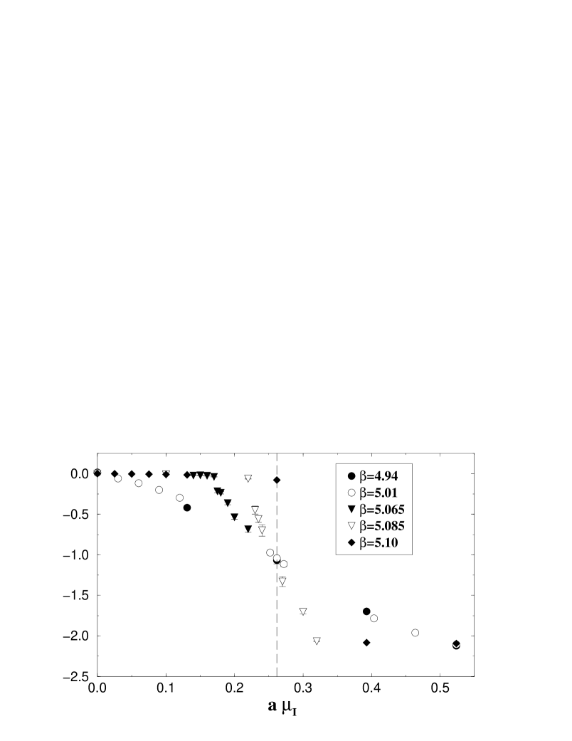
FIG. 1.: Average value of the Polyakov loop phase as a function of the imaginary chemical potential for different values of $\beta$. The vertical dashed line corresponds to $\theta=\mu_{I}/T=\pi/3$.

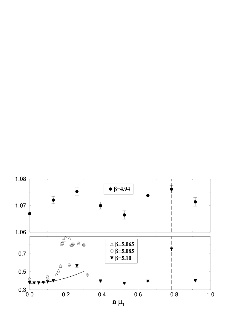
FIG. 2.: Average value of the chiral condensate as a function of the imaginary chemical potential for different values of $\beta$. The vertical dashed lines correspond to $\theta=\mu_{I}/T=(2k+1)\pi/3$. The continuous line in the lower picture is the result of a quadratic fit at small values of $a\mu_{I}$ obtained at $\beta=5.10$.

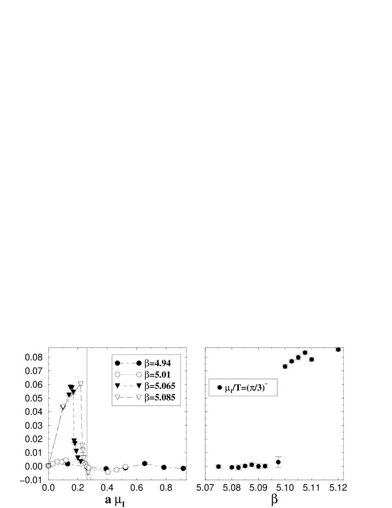
FIG. 3.: Imaginary part of the barion density as a function of $\mu_{I}$ for different values of $\beta$ (left–hand side), and as a function of $\beta$ at $\theta=\mu_{I}/T=\frac{\pi}{3}^{-}$ (right-hand side).

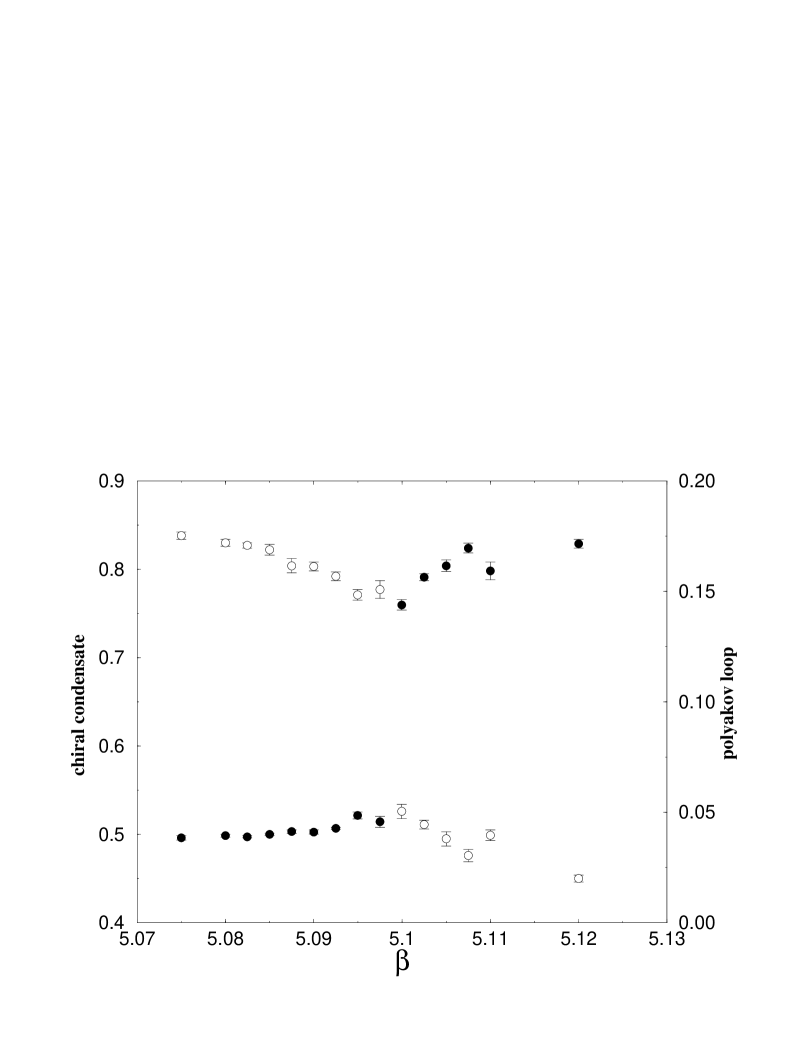
FIG. 4.: Chiral condensate (white circles) and absolute value of the Polyakov loop (black circles) as a function of $\beta$ for $\theta=\pi/3$. The sharp changes of the two quantities coincide with the location of endpoint of the RW critical line.

FIG. 5.: Sketch of the phase diagram in the $\mu_{I}$–$\beta$ plane. The filled cirles represents direct determinations of the chiral critical line location from our simulations. The rest of the chiral line has been obtained by interpolation and by exploiting the symmetries of the partition function.

FIG. 6.: The critical line of four flavor QCD, $m_{q}=.05$, in the $\mu^{2}$, $\beta$ plane. The dotted lines show the range of the results of the quadratic fits described in the text. The triangles are our results for the critical coupling from Table I. The results by Fodor and Katz (diamonds) are plotted for comparison.

FIG. 7.: O($\mu^{4}$) effects on the critical line of four flavor QCD. The solid line shows the results of a second order fit, the thin dotted line the results of a fourth order fit with first and second order coefficients constrained to their central values. The upper (lower) thick dotted line shows the results of a fourth order fit with the second coefficent constrained to its best value plus (minus) its error. See text for details.

FIG. 8.: The critical line of four flavor QCD, with $m_{q}=.05$. Result and error band are from $\beta=5.037(3)+0.96(10)\mu^{2}$ converted to physical units. The result (central line) is well approximated by $T=T_{c}\sqrt{(1-0.021\frac{\mu^{2}}{T_{c}^{2}}}$.

FIG. 9.: Scale invariant plot for the QCD critical line at high temperature, from imaginary chemical potential. Results for two flavors of staggered fermions (solid line) are from De Forcrand and Philipsen. The four flavor critical line (dotted) lies consistently below the two flavor one, the effect growing larger at larger density.

FIG. 10.: The analytic continuation to real chemical potential of the chiral condensate: the large bands are the errorband associated with the second Fourier coefficient. The symbols – triangles and squares – are printed only in the broken phase, for one (smaller errors) and two (larger errors) Fourier coefficient results. The critical chemical potential - where the symbols stops- has been inferred from Fig. 8 and related discussions. The results are consistent with a first order chiral transition

REFERENCES

- [1] M. G. Alford, K. Rajagopal and F. Wilczek, Phys. Lett. B 422 (1998) 247 R. Rapp, T. Schafer, E. V. Shuryak and M. Velkovsky, Phys. Rev. Lett. 81 (1998) 53; for a very recent review see e.g. F. Sannino, arXiv:hep-ph/0205007.
- [2] J. B. Kogut, H. Matsuoka, M. Stone, H. W. Wyld, S. H. Shenker, J. Shigemitsu and D. K. Sinclair, Nucl. Phys. B 225 (1983) 93; P. Hasenfratz and F. Karsch, Phys. Lett. B125, (1983) 308.
- [3] Recent reviews on the lattice approach to QCD in extreme environments include J. B. Kogut, arXiv:hep-lat/0208077; Z. Fodor, arXiv:hep-lat/0209101; K. Kanaya, arXiv:hep-ph/0209116.
- [4] F. Wilczek, Nucl. Phys. A 642, 1 (1998).
- [5] C. Bernard et al. [MILC Collaboration], arXiv:hep-lat/0209079; S. Gottlieb, W. Liu, D. Toussaint, R. L. Renken and R. L. Sugar, Phys. Rev. D 38 (1988) 2888; Phys. Rev. Lett 59 (1987) 2247; R.V. Gavai and S. Gupta, Phys. Rev. D64 (2001) 074506; Phys. Rev. D65 (2002) 094515; R.V. Gavai, S. Gupta and P. Majumbdar, Phys. Rev. D65 (2002) 054506.
- [6] Choe et al, Physical Review D65 (2002) 054501.
- [7] C.R. Allton et al, arXiv:hep-lat/0204010; S. Ejiri, C. R. Allton, S. J. Hands, O. Kaczmarek, F. Karsch, E. Laermann and C. Schmidt, arXiv:hep-lat/0209012; C. Schmidt, C. R. Allton, S. Ejiri, S. J. Hands, O. Kaczmarek, F. Karsch and E. Laermann, arXiv:hep-lat/0209009.
- [8] Z. Fodor and S. D. Katz, Phys. Lett. B 534 (2002) 87.
- [9] Z. Fodor and S. D. Katz, JHEP 0203 (2002) 014; Z. Fodor, S. D. Katz and K. K. Szabo, arXiv:hep-lat/0208078; F. Csikor, G.I. Egri, Z. Fodor, S.D. Katz, K.K. Szabo and A.I. Toth, arXiv:hep-lat/0209114.
- [10] E. Dagotto ,A. Moreo,R L. Sugar and D. Toussaint, Phys. Rev. B 41 (1990) 811.
- [11] A. Hasenfratz and D. Toussaint, Nucl. Phys. B 371 (1992) 539.
- [12] M. G. Alford, A. Kapustin and F. Wilczek, Physical Review D59 (1999) 054502.
- [13] M.-P. Lombardo, Nuclear Physics B (Proc. Suppl.) 83, (2000) 375.
- [14] A. Hart, M. Laine and O. Philipsen, Nucl. Phys. B586, (2000) 443; Phys. Lett. B505, (2001) 141.
- [15] O. Philipsen, arXiv:hep-ph/0110051.
- [16] P. de Forcrand and O. Philipsen, Nucl.Phys. B642 (2002) 290; arXiv:hep-lat/0209084.
- [17] M. D’Elia and M.-P. Lombardo, arXiv:hep-lat/0205022.
- [18] I.M. Barbour, S.E. Morrison, E.Klepfish, J.B.Kogut and M.-P. Lombardo, Nucl. Phys. B (Proc. Suppl.) 60A, (1998) 220.
- [19] Ph. de Forcrand, S. Kim and T. Takaishi, arXiv:hep-lat/0209126.
- [20] P. R. Crompton, Nucl. Phys. B 619 (2001) 499;arXiv:hep-lat/0209041.
- [21] A. Roberge and N. Weiss, Nuclear Physics B275 (1986) 734.
- [22] F.R. Brown et al, Physics Letters B251, (1990) 181.
- [23] G. Baym and N.D. Mermin, Jour. Math. Phys. 2 (1961) 232.
- [24] T.S. Evans, A. Gómez-Nicola, R.J. Rivers, D. A. Steer arXiv:hep-th/0204166,
- [25] B. Alles and E. M. Moroni, arXiv:hep-lat/0206028.
- [26] J. Ambjorn, K. N. Anagnostopoulos, J. Nishimura and J. J. Verbaarschot, arXiv:hep-lat/0208025.
- [27] B.P. Dolan, W. Janke, D.A. Johnston and M. Stathakopolous, arXiv:cond-mat/01053317.
- [28] S.Y. Kim, arXiv:cond-mat/0205451.
- [29] S. Hands, Nucl. Phys. Proc. Suppl. 106 (2002) 142.
- [30] S. Hands, Nucl. Phys. A 642 (1998) 228.
- [31] A. S. Vshivtsev, B. V. Magnitsky, V. C. Zhukovsky and K. G. Klimenko, Phys. Part. Nucl. 29 (1998) 523
- [32] K. G. Klimenko,Z. Phys. C37 (1988)457; S. Hands, A. Kocic and J. B. Kogut, Nucl. Phys. B 390 (1993) 355.
- [33] P.H. Damgaard, U.M. Heller, R. Niclausen and B. Svetisky Nucl. Phys. B 633 (2002) 97; P.M. Damgaard, arXiv:hep-lat/0110192.
- [34] M.A. Halasz, A.D. Jackson, R.E. Shrock, M.A. Stephanov and J.J.M Verbaarschot Phys. Rev. D 58 (1998) 096007.
- [35] B. Alles, M. D’Elia and A. Di Giacomo, Phys. Lett. B 483 (2000) 139.
- [36] see e g. F. Karsch, Lect. Notes Phys. 583 (2002) 209.