Monte Carlo studies of three-dimensional O(1) and O(4) theory related to BEC phase transition temperatures
Abstract
The phase transition temperature for the Bose-Einstein condensation (BEC) of weakly-interacting Bose gases in three dimensions is known to be related to certain non-universal properties of the phase transition of three-dimensional O(2) symmetric theory. These properties have been measured previously in Monte Carlo lattice simulations. They have also been approximated analytically, with moderate success, by large approximations to O() symmetric theory. To begin investigating the region of validity of the large approximation in this application, I have applied the same Monte Carlo technique developed for the O(2) model (Ref. [5]) to O(1) and O(4) theories. My results indicate that there might exist some theoretically unanticipated systematic errors in the extrapolation of the continuum value from lattice Monte Carlo results. The final results show that the difference between simulations and NLO large calculations does not improve significantly from to . This suggests one would need to simulate yet larger ’s to see true large scaling of the difference. Quite unexpectedly (and presumably accidentally), my Monte Carlo result for seems to give the best agreement with the large approximation among the three cases.
I Introduction
The computation of the phase transition temperature for dilute or weakly-interacting bose gases has attracted considerable interest. Due to the non-perturbative nature of long-distance fluctuations at the second-order phase transition at large distance, the calculation of corrections to the ideal gas formula for is non-trivial. In the dilute or weakly-interacting limit, the correction to the ideal gas result for a homogeneous gas can be parametrized as*** For a clean argument that the first correction is linear in , see Ref. [1]. For a discussion of higher-order corrections, see Refs. [2, 3].
| (1) |
where is the scattering length of the 2-particle interaction, is the number density of the homogeneous gas, is a numerical constant, and shows the parametric size of higher-order corrections. Baym et al. [1] have shown that the computation of can be reduced to a problem in three dimensional O() field theory. In general, O() field theory is described by the continuum action
| (2) |
where is an -component real field. I will focus exclusively on the case where has been adjusted to be at the order/disorder phase transition for this theory for a given value of the quartic coupling . The relationship to for Bose-Einstein condensation found by Baym et al. is that the constant in (1) is††† This is given separately in Ref. [1] as and the identification of as .
| (3) |
where , and
| (4) |
represents the difference between the critical-point value of for the cases of (i) non-zero and (ii) the ideal gas . Thus the computation of the first correction to due to interactions is related to the evaluation of in three-dimensional theory.
Having tuned to the phase transition, is then the single remaining parameter of the three-dimensional continuum theory (2). The dependence of (ultraviolet-convergent) quantities on is determined by simple dimensional analysis, and has dimensions of inverse length. The in (3) is dimensionless and so is a number independent of in the continuum theory. Monte Carlo simulations of this quantity in O(2) theory have given [4] and [5].
One of the few moderately successful attempts to approximate this result with an analytic calculation has been through the use of the large approximation. (But see also the 4th-order linear expansion results of Refs. [7]. For a brief comparison of the results of a wide spread of attempts to estimate , see the introduction to Ref. [6] and also Ref. [8].). The procedure is to calculate for O() theory in the limit that is arbitrarily large, and then substitute the actual value of interest into the result. The large result was originally computed at leading order in by Baym, Blaizot, and Zinn-Justin [9] and extended to next-to-leading order (NLO) in by Arnold and Tomášik [10], giving
| (5) |
Setting , one obtains , which is roughly 30% higher than the results obtained by Monte Carlo simulation of O(2) theory. Considering that has been treated as large in this approximation, the result is fairly encouraging.
The goal of the present work is to further explore the applicability of the large result (5) by testing it for other values of . I have applied to other O() models the same techniques used in Ref. [5] to simulate the O(2) model. In this paper I report the measurement of for the O(1) and O(4) theories. The final results, compared to the large approximations of (5), are given in table I.
As a byproduct of the analysis, I also report the measurement of the critical value of . The coefficient requires ultraviolet renormalization and so is convention dependent. In Table I, I report the dimensionless continuum values of with defined by dimensional regularization and modified minimal subtraction () renormalization at a renormalization scale set to . Among other things, this quantity can be related to the coefficient of the second-order () correction to [2, 11]. One can convert to other choices of the renormalization scale by the (exact) identity
| (6) |
| simulation | large | difference | simulation | |
|---|---|---|---|---|
| 1 | -0.000494(41) | -0.0004990 | - 1(8) % | 0.0015249(48) |
| 2 (Ref. [5]) | -0.001198(17) | -0.001554 | +30(2) % | 0.0019201(21) |
| 4 | -0.00289(18) | -0.003665 | +27(8) % | 0.002558(16) |
In section II, I briefly review the algorithm and the necessary background materials and formulas for improving the extrapolations of the continuum and infinite-volume limits. Most of the technical details can be found in Ref. [5]. Section III gives the simulation results and analysis. Section IV is the conclusion from comparing the numerical results with the NLO large calculation (5).
II Lattice Action and Methods
The action of the theory on the lattice is given by
| (7) |
where is the lattice size (not to be confused with the scattering length ). I will work on simple cubic lattices with cubic total volumes and periodic boundary conditions. As in Ref. [5] and as reviewed further below, the bare lattice operators and couplings (, , , ) are matched to the continuum, using results from lattice perturbation theory to improve the approach to the continuum limit for finite but small lattice spacing.
I shall use the improved lattice Laplacian
| (8) |
which (by itself) has errors, rather than the standard unimproved Laplacian
| (9) |
which has errors. Readers interested in simulation results with the unimproved kinetic term should see Ref. [23].
Because the only parameter of the continuum theory (2) at its phase transition is , the relevant distance scale for the physics of interest is of order by dimensional analysis. To approximate the continuum infinite-volume limit, one needs lattices with total linear size large compared to this scale and lattice spacing small compared to this scale. As a result, is the relevant dimensionless expansion parameter for perturbative matching calculations intended to eliminate lattice spacing errors to some order in . The analogous dimensionless parameter that will appear in the later discussions of the large volume limit is .
A Matching to continuum parameters
To account for the lattice spacing errors, I have adapted the perturbative matching calculations to improve lattice spacing errors given in Ref. [5], where the details of the calculations can be found. Here I will simply collect the results from that reference. The lattice action expressed in terms of continuum parameters is written in the form
| (10) |
The continuum approximate value for is theoretically expected to have the form
| (11) |
For the improved Laplacian, the matching calculations have been done to two-loop level () for , , and , and three loops () for , yielding
| (14) | |||||
| (15) | |||||
| (16) | |||||
| (17) | |||||
| (18) |
where, for the improved Laplacian (8),
| (20) | |||||
| (21) | |||||
| (22) | |||||
| (23) | |||||
| (24) | |||||
| (25) |
As shown in Ref. [5], the result of this improvement is that at fixed physical system size , the lattice spacing error of should be . However as will be shown in the following, my simulation results indicate that there might still exist some linear coefficients even after applying the formula (11). I assign an error to my continuum extrapolations that covers both linear and quadratic extrapolations.
This has produced about 10% systematic error in the final value of . The extrapolation of on the other hand has error, since no improvement has been made. Overall, the fitting formulas for the data taken at fixed are given as
| (27) | |||||
| (28) |
for a quadratic fit of , and
| (30) | |||||
| (31) |
for a linear fit of .
B Algorithm and Finite Volume Scaling
Working in lattice units () with the lattice action (10), I update the system by heatbath and multi-grid methods [21]. At each level of the multi-grid update, I perform over-relaxation updates. Statistical errors are computed using the standard jackknife method.
The strategy is to vary at fixed to reach the phase transition point. In order to define a nominal “phase transition” point in finite volume, I use the method of Binder cumulants [22]. The Binder cumulant of interest is defined by
| (32) |
where is the volume average of ,
| (33) |
The nominal phase transition is defined as occurring when , where is a universal value which improves convergence to the infinite volume limit. depends on the shape and boundary conditions of the total lattice volume but not on the short distance structure. For cubic lattice volumes with periodic boundary conditions, for O(1) [16] and for O(4) [17]. I have checked that the errors on are not significant for the purposes of this application. Therefore I have used the central values for the nominal .
In practice, it never happens that the simulation is done precisely at the where . I instead simply simulate at some close to it. I then use canonical reweighting of the time series data to analyze ’s near and determine and at .
A renormalization group analysis of the scaling of finite volume errors shows that, when the method of Binder cumulants is used, the values of and scale at large volumes as [5]
| (35) |
| (36) |
for fixed . Here is the dimension of space, , and and are the standard O() critical exponents associated with the correlation length and corrections to scaling, respectively. The values of the exponents that I have used are‡‡‡A nice review and summary of the critical exponents can be found in [12]. For the case of O(1), we have used their summarized values of and based on the calculation from High Temperature(HT) expansion technique and Monte Carlo simulations. For comparison, some experimental results for are: [13], [14]. For O(4), Monte Carlo simulation for gives: [15](used by us), [18]. From HT expansion: [19]; from -expansion 0.737(8)[20]. For , the only MC simulation result is (without quotation of error) from [18]. Ref. [20] gives (d=3 exp.) and 0.795(30) (-exp.). We have chosen the value to cover both of the errors for .
| (37) |
The large volume scaling of depends only on , which have errors 0.1% in both cases. They have a negligible effect on my final results. On the other hand, for the case of , the large volume scaling depends on both and . I will show that the errors of do have effects on the large volume errors of . They are included in the final results.
For a discussion of higher-order terms in the large volume expansion, see Ref. [5], but the above will be adequate for this application. I will fit the large data to the leading scaling forms (II B) to extract the infinite volume limit.
The basic procedure for extracting simultaneously the and limits of my result will be as follows. (i) I first fix a reasonably small value of of , take data for a variety of sizes (to as large as practical), and then extrapolate the size of finite volume corrections, fitting the coefficients and of the scaling law (II B). (ii) Next, I instead fix a reasonably large physical size and take data for a variety of (to as small as practical), and extrapolate the continuum limit of our results at that , which corresponds to fitting and of (II A, II A). (iii) Finally, I apply to the continuum result of step (ii) the finite volume correction for determined by step (i). In total, I have
| (38) | |||||
| (39) |
There is a finite lattice spacing error in the extraction of the large volume correction (i.e. and ). In Ref. [5], it is argued that this source of error is formally high order in and so expected to be small.
III Simulation Results
A O(1) Results for
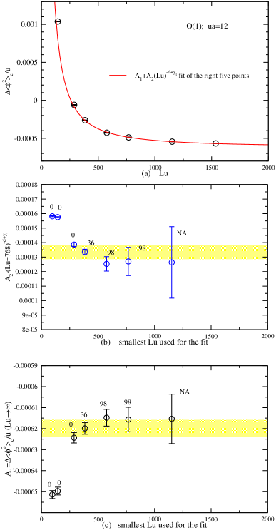
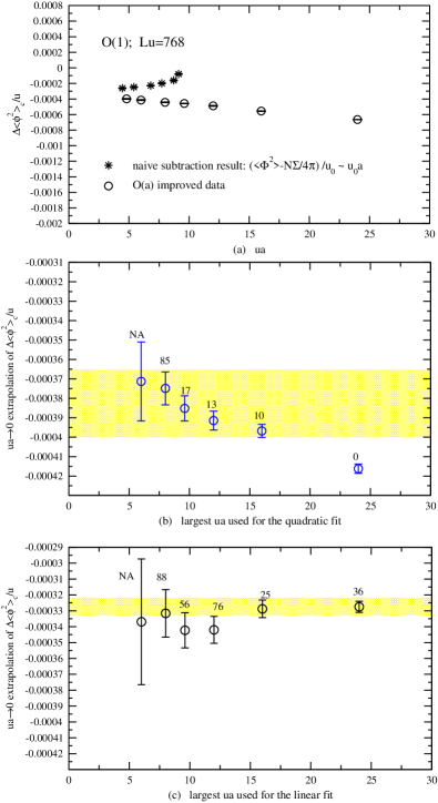
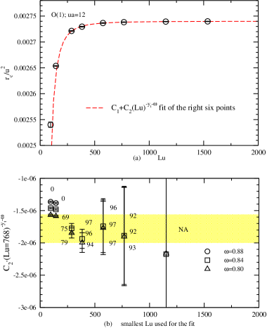
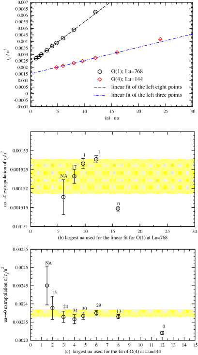
There is a practical tradeoff between how large one can take the system size in order to reach the large volume limit versus how small one can take in order to reach the continuum limit. Fig. 1(a) and the lower points (circles) in 2(a) show, respectively, the dependence at and the dependence at for in the O(1) model. From the dependence, we can see that is a reasonably large value of — the finite volume corrections are moderately small. From the dependence, we can see that is reasonably small.
Fig. 1(b) shows the size at when fitting the dependence of Fig. 1(a) to the scaling form (35). The result of the fit, and its associated confidence level, depends on how many points are included in the fit. Percentage confidence levels are shown in the figure. My procedure will be to determine the best values of the fit parameters by including as many points as possible while maintaining a reasonable confidence level. Then to assign an error, I use the statistical error from including one less point in the fit. This will help avoid the underestimation of systematic errors. The resulting estimate 0.0001335(50) of the finite volume correction is depicted by the shaded bar in Fig. 1(b) and collected in Table II. The corresponding best fit is shown as the solid line in Fig. 1(a). Even though there is no direct use of it, I show for completeness the fit parameter in Fig. 1(c), which corresponds to the infinite-volume value of at .
Having found the large volume extrapolated values, I will now move on to the limit for at a fixed physical volume . Theoretically, from the argument of Ref. [5], if one uses the improved formula (11) to obtain the continuum approximated , the remaining lattice error should be .
The circular data in Fig. 2(a) show the improved simulation results by using Eq. (11) . First I have tried a quadratic fit with the form . The fitting results for are given by Fig. 2(b). One can see while a three-point () fit gives an impressive C.L. of 85%, including the fourth point () reduces the C.L. to 17%. However, adding two more points keeps the C.L. above 10%. Due to this feature, it is hard to determine the last point that should be fit to the quadratic formula. Instead, I assigned the value to cover all the , , and C.L.s which gives -0.000383(17). The result is indicated by the shaded area.
The poor behavior of the quadratic fit makes one wonder if the data is actually more “linear” than “quadratic.” To check this, I re-fit the circular data using a linear function (30). The results are shown in Fig. 2(c). Surprisingly, I can fit all the data points with a very good C.L.. The extrapolated value in this case is -0.0003275(55), which is very different from the quadratic fit result. The obvious linear behavior of the data seem to indicate that there might be some residual coefficient in Eq. (11) that has not been accounted for. Given this uncertainty, I have used both the linear and quadratic extrapolated results, combined with the error due to the finite lattice size to obtain two continuum values (Table II). They differ by about 10%, which is considered my systematic error. The final result is assigned to cover both results and is tabulated in Tables II and I.§§§In Ref. [5], for the case of O(2) model, the fixed data are fitted by quadratic functions only. The data can be fitted also by a linear function. The data on the other hand can be fitted by only a quadratic function for the first four points. However if one takes off the smallest point, the rest four points can be fitted very well by a straight line too. This might indicate that there could be also some linear coefficients in the O(2) theory. For more discussions on this possible linear coefficient see Ref. [23].
As a comparison, I have also shown the naive subtracted result given by vs. the unimproved as the scale based on the same simulation (the stars in Fig. 2(a)). One can see that the finite lattice spacing errors is more explicit with the stars, corresponding to the unimproved data, than that of the circles, corresponding to the improved ones (using (11)). Theoretically data have and dependences on .
B and O(4) Results
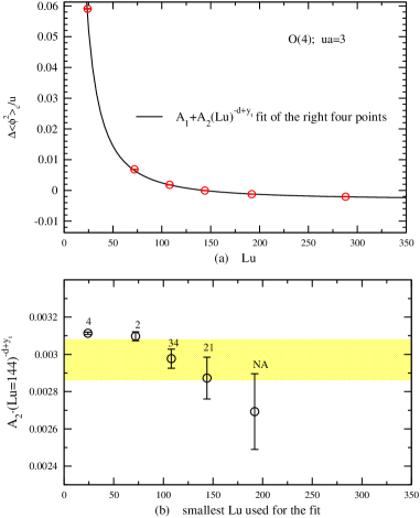
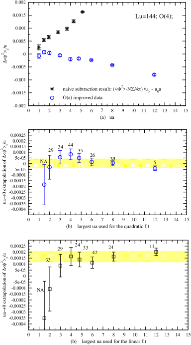
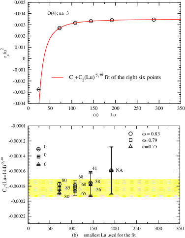
Figs. 3 and 4 show similar curves for the O(4) model, where we have taken and as a reasonably large size and reasonably small lattice spacing. It’s worth noting the large limit predicts that the distance scale that characterizes the physics of interest should scale as . That leads one to expect that the upper limit for “reasonably small” values of and lower limit for “reasonably large” values of should scale roughly as .
The fitting proceeds as in the O(1) case. For the -fixed data of (Fig. 4), I have again fitted the data with both linear and quadratic functions. Both the quadratic fit and the linear fit can go up to while keeping good C.L.s. However their extrapolations are also different (see Fig. 4 and Table II for the fitting results). The final continuum value is assigned to cover both extrapolations.
The analysis of the result for in both the O(1) and O(4) models is much the same (Figs. 5–7). For the large volume extrapolations, since the critical exponent has a larger uncertainty (, I have used three different values of (maximum, central, minimum) for both O(1) and O(4)’s cases. The final results of the value cover all the three different extrapolated values. This difference results in about of the error quoted in the final results for . For the fixed data, since there is no improvement of errors, the continuum extrapolation of the data taken at fixed are fitted to linear behavior in , following (28 or 31). The fitting results are again summarized in Tables I and II.
| fit | fit | fit | ||||||
| final | ||||||||
| 1 | (768,12) | -0.0006199(40) | 0.0001335(50) | -0.000383(17) | -0.003275(55) | -0.000517(18) | -0.0004610(74) | -0.000494(41) |
| 4 | (144,3) | -0.003023(92) | 0.002978(92) | 0.000007(26) | 0.000163(37) | -0.002971(96) | -0.002815(99) | -0.00289(18) |
| fit | fit | |||||||
| 1 | (768,12) | 0.00274001(28) | -0.00000178(22) | 0.0015231(48) | 0.0015249(48) | |||
| 4 | (144,3) | 0.0035035(62) | -0.000183(12) | 0.002375(10) | 0.002558(16) | |||
IV Conclusion
Fig. 8 and Table II show a comparison of the simulation results for with the NLO result (5) for . The cases are from this paper. The result of O(2) model is taken from Ref. [5].¶¶¶If one also considers the systematic uncertainty in the extrapolation in Ref. [5], then the result for O(2) should have a higher systematic uncertainty. In the figure, I have actually plotted , where the explicit factor of factors out the leading-order dependence on as . Amusingly, the large estimate for seems to be the most accurate of the three cases. This is presumably an accident—the result of the large approximation just happens to be crossing the set of actual values near . From Eq. (5), the error of the for should scale as , but there is clearly no sign of such behavior between and . This might indicate that is still too small for the error in the large approximation to scale properly. It would be interesting to numerically study yet higher such as or to attempt to verify the details of the approach to the large limit.
For the systematic error due to the possible linear behavior in the extrapolation of , so far no theoretical reasoning is found. It would be interesting to reinvestigate the matching calculations given in Ref. [5].
Acknowledgements.
I would like to thank the physics department of the University of Virginia for providing me the opportunity and support for this research work. The work was supported, in part, by the U.S. Department of Energy under Grant No. DE-FG02-97ER41027. I am especially grateful to P. Arnold for his valuable guidance and assistance throughout the research work.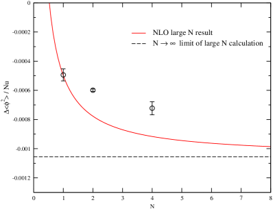
A Tabulated Data
Tables A and A are a collection of all the data reported in this paper. The standard integrated decorrelation time for a single operator is defined
| (A1) |
where
| (A2) |
is the auto-correlation function associated with the operator . In practice the sum in (A1) is cut-off when first drops below because of the statistical fluctuation in . The nominal decorrelation time listed in Tables A and A is the largest value of the various operators required in the computations of the Binder cumulant and by using the canonical reweighting method ([5]).
| O(1) | ||||||
|---|---|---|---|---|---|---|
| 8. | 8 | 1. | -0.01975(18) | 0.14599(50) | 0.8 | 61617 |
| 12. | 12 | 1. | -0.00901(12) | 0.07718(41) | 0.9 | 58809 |
| 24. | 8 | 3. | -0.001194(44) | 0.02577(14) | 1.1 | 47134 |
| 36. | 12 | 3. | 0.000437(31) | 0.01332(11) | 1.1 | 46288 |
| 48. | 16 | 3. | 0.001059(10) | 0.008149(54) | 1.1 | 44135 |
| 96. | 8 | 12. | 0.0025401(52) | 0.002530(23) | 2.5 | 20188 |
| 144. | 12 | 12. | 0.00265373(60) | 0.0010371(26) | 2.3 | 590789 |
| 192. | 32 | 6. | 0.0020919(35) | 0.000446(20) | 3.5 | 7175 |
| 288. | 24 | 12. | 0.00272132(81) | -0.0000604(44) | 4.3 | 53716 |
| 384. | 32 | 12. | 0.00272961(71) | -0.0002622(36) | 5.8 | 19281 |
| 576. | 48 | 12. | 0.00273662(70) | -0.0004271(50) | 11.3 | 6731 |
| 768. | 128 | 6. | 0.00213384(75) | -0.0004142(63) | 4795 | |
| 768. | 160 | 4.8 | 0.00201051(74) | -0.0003987(61) | 1643 | |
| 768. | 32 | 24. | 0.00416985(16) | -0.0006645(23) | 3.7 | 13690 |
| 768. | 48 | 16. | 0.00315905(45) | -0.0005548(39) | 11.5 | 8800 |
| 768. | 64 | 12. | 0.00273822(48) | -0.0004886(51) | 8.9 | 22219 |
| 768. | 80 | 9.6 | 0.00249587(61) | -0.0004567(42) | ∥∥∥Numbers with means the simulation data are collected every 10 sweeps. | 4545 |
| 768. | 96 | 8. | 0.00233612(56) | -0.0004429(39) | 15260 | |
| 1152. | 96 | 12. | 0.00273936(42) | -0.0005441(33) | 3480 | |
| 1536. | 128 | 12. | 0.00273977(41) | -0.0005679(33) | 1411 | |
REFERENCES
- [1] G. Baym, J.-P. Blaizot, M. Holzmann, F. Laloë, and D. Vautherin, Phys. Rev. Lett. 83, 1703 (1999).
- [2] P. Arnold, G. Moore, B. Tomik, Phys. Rev. A 65, 013606 (2002) .
- [3] M. Holzmann, G. Baym, and F. Laloë, Phys. Rev. Lett. 87, 120403 (2001).
- [4] V. A. Kashurnikov, N. V. Prokof,ev, and B. V. Svistunov, Phys. Rev. Lett. 87, 120402 (2001); 87, 160601 (2001).
- [5] P. Arnold, G. Moore, Phys. Rev. E 64, 066113 .
- [6] P. Arnold, G. Moore, Phys. Rev. Lett. 87, 120401 (2001) .
- [7] F. F. de Sourza Cruz, M. B. Pinto, R. O. Ramos, and P. Sena, Phys. Rev. A 65, 053613 (2002); E. Braaten and E. Radesci, cond-mat/0206186.
- [8] G. Baym, J.-P. Blaizot, M. Holzmann, F. Laloë, and D. Vautherin, cond-mat/0107129.
- [9] G. Baym, J.-P. Blaizot, and J. Zinn-Justin, Europhys. Lett. 49, 150 (2000).
- [10] P. Arnold, B. Tomášik, Phys. Rev. A 62, 063604 (2000).
- [11] P. Arnold, B. Tomášik, Phys. Rev. A 64, 053609 (2000).
- [12] A. Pelissetto and E. Vicari , cond-mat/0012164 (2002)
- [13] D. M. Sullivan, G. W. Neilson, H. E. Fisher, A. R. Rennie, J. Phys.: Condens. Matter 12, 3531 (2000).
- [14] B. H. Chen, B. Payandeh, M. Robert, Phys. Rev. E. 62, 2369 (2000); 64, 042401 (2001).
- [15] H. G. Ballesteros, L. A. Fernández, V. Martin-Mayor, A. Muñoz Sudupe Phys. Lett. B 387 (1996).
- [16] H. Blöte, E. Luijten, J. Heringa, J. Phys. A: Math. Gen. 28, 6289 (1995); H. G. Ballesteros, L. A. Fernández, et al, J. Phys. A: Math. Gen. 32, 1 (1999).
- [17] M. Hasenbusch, J. Phys. A: Math. Gen. 34, 8224 (2000) .
- [18] M. Hasenbusch, Int. J. Mod. Phys. C 12, 911 (2001).
- [19] P. Butera, M. Comi, Phys. Rev. B 56, 8212 (1997) .
- [20] R. Guida, J. Zinn-Justin, J. Phys. A 31, 8103 (1998).
- [21] J. Goodman, A. D. Sokal, Phys. Rev. D 40, 2035 (1989) .
- [22] K. Binder, Phys. Rev. Lett. 47, 693 (1981); Z. Phys. B 43, 119 (1981) .
- [23] X. Sun, Ph.D thesis, Univ. of Virginia (2002) .