Abstract: We present results of numerical simulations of the 3+1$d$ Nambu – Jona-Lasinio model with a non-zero baryon chemical potential $\mu$, with particular emphasis on the superfluid diquark condensate and associated susceptibilities. The results, when extrapolated to the zero diquark source limit, are consistent with the existence of a non-zero BCS condensate at high baryon density. The nature of the infinite volume and zero temperature limits are discussed.

1 Introduction

Colour superconductivity (CSC) at low temperature and high baryon number density is one of the most intensively studied topics in QCD thermodynamics (for recent reviews see [1]). The basic idea is that diquark pairs at the Fermi surface in quark matter become bound and condense in a relativistic analogue of the BCS mechanism for electronic superconductivity [2]. Because of the strong attractive $qq$ force in QCD, however, estimates of the energy gap $\Delta$, which opens up at the Fermi surface, can be as large as 100MeV [3], with potentially important consequences for the physics of compact stars. For instance, one intriguing possibility is that pairing between quarks with differing Fermi momenta may lead to a crystalline phase in which translational invariance of the ground state is spontaneously broken [4].

Analytic approaches to the problem, however, are restricted either to asymptotically high (and phenomenologically irrelevant) densities where perturbative QCD is applicable, or to self-consistent treatments of model theories which capture some but not all relevant physics. A first principles calculation using lattice QCD remains elusive due to the difficulties of performing Monte Carlo simulations with baryon chemical potential $\mu\not=0$. There are, however, simpler models which are simulable. Two Colour QCD is a confining theory in which the lightest baryons are bosonic $qq$ states. At high density its ground state has a gauge invariant condensate $\langle qq\rangle\not=0$ which spontaneously breaks baryon number symmetry leading to superfluidity. Because of the absence of a Fermi surface, however, the phenomenon far more closely resembles a standard Bose-Einstein condensation, and is well-described by chiral perturbation theory [5]; this picture is confirmed by lattice simulation [6, 7]. The NJL model [8], by contrast, is a strongly-interacting model with fermionic excitations but no confinement. It can be treated by self-consistent analytic methods and has been applied to CSC [3] as well as more general issues in low-energy QCD [9].

The NJL model with $\mu\not=0$ has also been simulated, on a 2+1 dimensional lattice. Although evidence for $qq$ pairing has been found in the scalar isoscalar channel [10], BCS condensation does not take place [11], the argument being that long-wavelength fluctuations in the phase of the condensate wavefunction wipe out long range order. Because phase coherence remains, however, superfluidity is realised in an unconventional “thin film” fashion. This picture, related to the low dimensionality of the system, is essentially non-perturbative and would not be exposed by use of self-consistent methods. It points to the potential importance of fully non-perturbative treatments of even simple models in attempts to understand CSC. In this Letter we extend the lattice analysis of [11] to the NJL model in 3+1$d$, motivated by (i) the possibility for a genuine BCS condensation in this case, and (ii) the model’s phenomenological relevance. In the following sections we review the lattice formulation of NJL, show how lattice parameters may be chosen to match low energy QCD, and then report results from simulations with $\mu\not=0$, paying particular attention to diquark observables. We will show that the high density phase is qualitatively different to that observed in 2+1$d$ and far more closely resembles a conventional BCS superfluid; however, some issues concerning the thermodynamic limit need to be resolved before this conclusion can become definitive.

2 Lattice Model and Parameter Choice

The model studied here is the 3+1$d$ version of that studied in [11]. In particular it has the action

$$S={\bf\Psi}^{tr}{\cal A}{\bf\Psi}+\frac{2}{g^{2}}\sum_{\tilde{x}}\left(\sigma^{2}+\vec{\pi}.\vec{\pi}\right),$$ (1)

where $g^{2}$ is the four-fermi coupling constant, the bispinor ${\bf\Psi}$ is written in terms of staggered isospinor fermionic fields via ${\bf\Psi}^{tr}=(\overline{\chi},\chi^{tr})$, and the auxiliary bosonic fields $\sigma$ and $\vec{\pi}$, which live on sites $\tilde{x}$ of a dual lattice, are introduced in the standard way. Written in the Gor’kov basis the fermion matrix is

$${\cal A}=\frac{1}{2}\left(\begin{array}[]{cc}\overline{\jmath}\tau_{2}&M\\ -M^{tr}&j\tau_{2}\end{array}\right),$$ (2)

where the matrix $M$ is defined by

$$M^{pq}_{xy} = \frac{1}{2}\delta^{pq}\left[\left(e^{\mu}\delta_{yx+\hat{0}}-e^{-\mu}\delta_{yx-\hat{0}}\right)+\sum_{\nu=1}^{3}\eta_{\nu}(x)\left(\delta_{yx+\hat{\nu}}-\delta_{yx-\hat{\nu}}\right)+2m_{0}\delta_{xy}\right]$$ (3)

$$+ \frac{1}{16}\delta_{xy}\sum_{\left<\tilde{x},x\right>}\left(\sigma(\tilde{x})\delta^{pq}+i\epsilon(x)\vec{\pi}(\tilde{x}).\vec{\tau}^{pq}\right),$$

$m_{0}$ is the bare quark mass and the symbols $\eta_{\nu}(x)$, $\epsilon(x)$ are the phases $(-1)^{x_{0}+\dots+x_{\nu-1}}$ and $(-1)^{x_{0}+x_{1}+x_{2}+x_{3}}$ respectively. The Pauli matrices $\vec{\tau}$ are normalised such that ${\rm tr}(\tau_{i}\tau_{j})=2\delta_{ij}$, and $\left<\tilde{x},x\right>$ represents the set of 16 dual lattice sites neighbouring $x$. The diquark sources $j$ and $\overline{\jmath}$ are introduced to allow us to measure the diquark condensate and play the same ${\rm r\hat{o}le}$ as a bare quark mass in the lattice estimation of the chiral condensate. (NB. The sources used are greater than those in [11] by a factor of 2, which allows us to identify them with Majorana fermion masses.) We simulate the action (1) using a hybrid Monte Carlo (HMC) algorithm which uses a functional weight $\mbox{det}{\cal AA^{\dagger}}$, thus doubling the number of fermion degrees of freedom, but which has the advantage of of being exact. We treat the diquark terms in the partially quenched approximation, ie. the sources $j$ and $\overline{\jmath}$ are set to zero during the HMC update of the bosonic fields, but are made non-zero during the measurement of diquark observables. Field theoretically, this means that the formation of virtual diquark pairs in the vacuum is suppressed. This approach has the advantage that one can examine many source strengths for only one (computationally expensive) chain of field evolutions.

Our formulation employs staggered quarks, which, although preserving some of the model’s continuum chiral symmetry, increase the number of quark degrees of freedom by a factor $N_{c}=4$. As the NJL model has no gauge degrees of freedom we interpret these doublers phenomenologically as “colours”. The model is therefore an effective $N_{f}=2$, $N_{c}=4$ QCD-like theory. It should be stressed, however, that a diquark condensate in this model breaks global rather than local symmetries, hence physically giving rise to superfluid rather than superconducting behaviour. The continuum limit of the model yields the Lagrangian density [12, 6]

$${\cal L}_{{\rm cont}} = \overline{\psi}_{i}\left(\partial/+m_{o}+\mu\gamma_{0}\right)\psi_{i}-\frac{g^{2}}{2}\left[\left(\overline{\psi}_{i}\psi_{i}\right)^{2}-\left(\overline{\psi}_{i}\gamma_{5}\otimes\vec{\tau}\otimes\gamma_{5}\psi_{i}\right)^{2}\right]$$ (4)

$$+\frac{1}{2}\left[j\left({\psi_{i}}^{tr}C\gamma_{5}\otimes\tau_{2}\otimes C\gamma_{5}\psi_{j}\right)+\overline{\jmath}\left(\overline{\psi}_{i}C\gamma_{5}\otimes\tau_{2}\otimes C\gamma_{5}{\overline{\psi}_{j}}^{tr}\right)\right],$$

which in the limits $m_{0}\rightarrow 0$ and $j,\bar{\jmath}\to 0$ recovers the ${\rm SU}(N_{f})_{L}\otimes{\rm SU}(N_{f})_{R}$ chiral and ${\rm U}(1)_{B}$ baryon number symmetries of QCD respectively. In the tensor products the first matrix acts on spinor, the second on isopinor, and the third on “colour” indices.

Due to the point-like nature of the four-fermi interaction, the NJL model has no interacting continuum limit for $d\geq 4$, leaving physics dependent on the UV regularisation employed [9, 12]. In order to ensure we simulate in a physically plausible regime, we employ the methods used in [9] to match our model’s parameters to low energy, vacuum phenomenology, taking advantage of the fact that a perturbative expansion in $1/N_{c}$ is possible in four-fermi theories. We calculate quantities analytically to leading order in $1/N_{c}$, the Hartree approximation, using staggered quark propagators defined on a $L_{s}^{3}\times L_{t}/2^{4}$ Euclidean blocked lattice [13], with periodic boundary conditions in spatial dimensions and anti-periodic boundary conditions in the temporal dimension. The momentum loop integrals are discretised using mode sums and taken to the limit $V^{-1}\rightarrow 0$ where $V=L_{s}^{3}L_{t}$.

In particular we calculate the dimensionless ratio between the pion decay rate $f_{\pi}$ and the constituent quark mass $m^{*}=\Sigma+m_{0}$, where $\Sigma\equiv\langle\sigma\rangle$.

$$\frac{f_{\pi}}{m^{*}}=\sqrt{2N_{c}N_{f}}\int^{\frac{\pi}{2}}_{-\frac{\pi}{2}}{\frac{d^{4}p}{\left(2\pi\right)^{4}}\frac{\cos{2p_{\nu}}}{\left[\tilde{p}^{2}+\left(am^{*}\right)^{2}\right]^{2}}}\sqrt{\int^{\frac{\pi}{2}}_{-\frac{\pi}{2}}{\frac{d^{4}p}{\left(2\pi\right)^{4}}\frac{1}{\left[\tilde{p}^{2}+\left(am^{*}\right)^{2}\right]^{2}}}},$$ (5)

where $\tilde{p}^{2}=\sum_{\nu=0}^{3}{\sin^{2}p_{\nu}}$.

Fixing $f_{\pi}$ to its experimental value of 93MeV and $m^{*}$ to a physically reasonable 350MeV, we extract a dimensionless quark mass of $am^{*}=0.3251$, where $a$ is the spacing between lattice points, which in this section we will not set to unity. Calculating the product of $\Sigma$ and the dimensionless inverse coupling $\beta=a^{2}/g^{2}$,

$$\Sigma\beta a=2N_{c}N_{f}am^{*}\int^{\frac{\pi}{2}}_{-\frac{\pi}{2}}\frac{d^{4}p}{\left(2\pi\right)^{4}}\frac{1}{\tilde{p}^{2}+\left(am^{*}\right)^{2}}=0.1826,$$ (6)

allows us to derive that $\beta=0.1826/{\left(0.3251-am_{0}\right)}$.

Finally, calculating the mass of the pion $m_{\pi}$ allows us to fix $m_{0}$, and therefore $\beta$. In the Hartree approximation the pion propagator can be written as a series of connected bubble diagrams

$$\frac{a^{2}}{\tilde{k}^{2}+{\left(am_{\pi}\right)}^{2}}=\frac{g^{2}}{2}-\frac{g^{2}\Pi_{\rm{ps}}(\tilde{k}^{2})g^{2}}{4}+\frac{g^{2}\Pi_{\rm{ps}}(\tilde{k}^{2})g^{2}\Pi_{\rm{ps}}(\tilde{k^{2}})g^{2}}{8}-\ldots=\frac{g^{2}}{2+g^{2}\Pi_{\rm{ps}}(\tilde{k}^{2})}$$ (7)

in terms of the vacuum polarisation of the pion

$$\Pi_{\rm{ps}}\left(\tilde{k}^{2}\right)=-2\left(\frac{m^{*}-m_{0}}{m^{*}g^{2}}\right)\\ +2N_{c}N_{f}{\tilde{k}^{2}\over a^{2}}I\left(\tilde{k}^{2}\right),$$ (8)

where

$$I\left(\tilde{k}^{2}\right)=\int^{\frac{\pi}{2}}_{-\frac{\pi}{2}}{\frac{d^{4}p}{\left(2\pi\right)^{4}}\frac{1}{\left[\sum_{\mu}{\sin^{2}{\left(p+\frac{k}{2}\right)_{\mu}}}+{\left(am^{*}\right)}^{2}\right]\left[\sum_{\nu}{\sin^{2}{\left(p-\frac{k}{2}\right)_{\nu}}}+{\left(am^{*}\right)}^{2}\right]}},$$ (9)

$p_{\mu}$ is the loop momentum shifted to be independent of $a$, and $k_{\mu}/a$ is the physical momentum of the pion. The fact that there is a pole in (7) at $\tilde{k}^{2}=-a^{2}m_{\pi}^{2}$ combined with (9) allows us to write

$$m_{\pi}^{2}=\frac{m_{0}}{m^{*}}\left.\frac{1}{N_{c}N_{f}g^{2}I\left(\tilde{k}^{2}\right)}\right|_{\tilde{k}^{2}=-a^{2}m_{\pi}^{2}}.$$ (10)

A bare quark mass of $am_{0}=0.002$ leads to a phenomenologically acceptable pion mass of 138MeV and implies an inverse coupling $\beta=0.565$. Finally, as we know both $am^{*}$ and $m^{*}$ we can extract the lattice spacing in the large-$N_{c}$ approximation, with the result $a^{-1}=1076{\rm MeV}$, or $a\sim 0.2{\rm fm}$.

3 Equation of State

As has been previously discussed, in the limit $m_{0}\rightarrow 0$ the NJL model has an exact ${\rm SU}(2)_{L}\otimes{\rm SU}(2)_{R}$ chiral symmetry, which for sufficiently large $g^{2}$ is spontaneously broken in the vacuum to ${\rm SU}(2)_{{\rm isospin}}$, leading to a dynamically generated quark mass $m^{*}=\Sigma$, and 3 massless Goldstone pions. In the presence of a baryon chemical potential $\mu$ the symmetry is approximately restored as $\mu$ is increased through some onset scale $\mu_{o}\sim\Sigma$, with the order of the transition being highly sensitive to the parameters employed [9].

We determine the nature of this transition in our physically reasonable regime by studying the order parameter, the chiral condensate $\left<\overline{\chi}\chi\right>$, defined by

$$\left<\overline{\chi}\chi\right>=\frac{1}{V}\frac{\partial\ln{\cal Z}}{\partial m_{{}_{0}}},$$ (11)

where ${\cal Z}$ is the partition function. We also study the baryon number density $n_{B}$;

$$n_{B}=\frac{1}{2V}\frac{\partial\ln{\cal Z}}{\partial\mu}.$$ (12)

These are calculated as functions of $\mu$, both in the large-$N_{c}$ limit and by numerical lattice simulation, using a repeated stochastic estimator for the diagonal elements of the inverse fermion matrix. We use a HMC algorithm with $\beta=0.565$, $m_{0}=0.002$ on $L_{s}^{3}\times L_{t}$ lattices with $L_{s}=L_{t}=12$, $16$ and $20$ for various values of $\mu$, as well as on lattices with $L_{s}\neq L_{t}$ at $\mu=1.0$. Approximately 500 equilibrated configurations separated by HMC trajectories of mean length 1.0 were generated in each run, with measurements carried out on every other configuration. Statistical errors were calculated using a jackknife estimate.

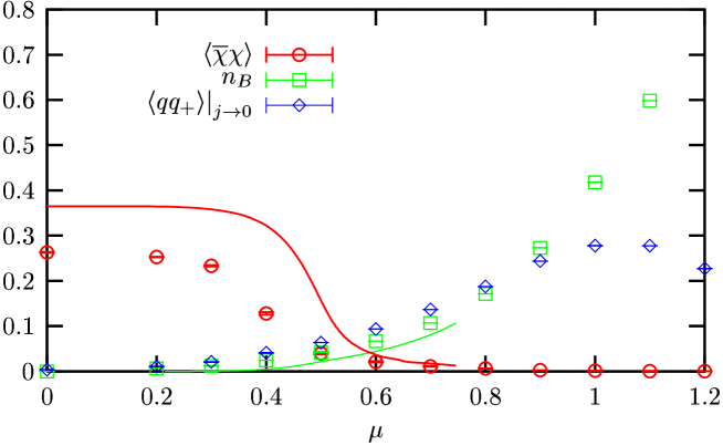
Figure 1: Chiral condensate and number density as functions of $\mu$ extrapolated to $V^{-1}\rightarrow 0$ showing both the large-$N_{c}$ solution (solid curve) and lattice results (points). The diquark condensate is plotted in the zero temperature, zero-source limit.

Our results are shown in Fig. 1, where the solid curve denotes the solution in the Hartree approximation, where $\langle\bar{\chi}\chi\rangle=2\Sigma\beta$, and the points denote lattice results. We carried out a linear extrapolation in $V^{-1}$ to the thermodynamic limit. To leading order in $1/N_{c}$ chiral symmetry is approximately restored via a crossover between 0.4${\lower 2.0pt\hbox{$\scriptstyle<$}\atop\raise 4.0pt\hbox{$\scriptstyle\sim$}}$$\mu$${\lower 2.0pt\hbox{$\scriptstyle<$}\atop\raise 4.0pt\hbox{$\scriptstyle\sim$}}$0.6. The lattice data agree qualitatively with this although both $\langle\bar{\chi}\chi\rangle$ and $\mu_{o}$ are about 30% smaller, which we attribute to ${\cal O}(1/N_{c})$ corrections. $n_{B}$ increases approximately as a power of $\mu$.

4 Diquark Condensation

4.1 Observables

In order to explore the possibility of a U(1)_B-violating BCS phase at high $\mu$ we study both the diquark order parameter and susceptibilities [11]. The operators

$$qq_{\pm}(x)=\chi^{tr}\frac{\tau_{2}}{4}\chi(x)\pm\overline{\chi}\frac{\tau_{2}}{4}\overline{\chi}^{tr}(x)$$ (13)

allow us to define the diquark condensate as

$$\left<qq_{+}\right>=\frac{1}{V}\frac{\partial\ln{\cal Z}}{\partial j_{+}},$$ (14)

where $j_{\pm}=j\pm\overline{\jmath}$. We also define the susceptibilities

$$\chi_{\pm}=\sum_{x}\left<qq{{}_{\pm}}(0)qq_{{}_{\pm}}(x)\right> = \frac{1}{16}\sum_{x}\left<\chi^{tr}\tau_{2}\chi(0)\chi^{tr}\tau_{2}\chi(x)+\overline{\chi}\tau_{2}\overline{\chi}^{tr}(0)\overline{\chi}\tau_{2}\overline{\chi}^{tr}(x)\right>$$ (15)

$$\hskip 15.93347pt\pm\left<\chi^{tr}\tau_{2}\chi(0)\overline{\chi}\tau_{2}\overline{\chi}^{tr}(x)+\overline{\chi}\tau_{2}\overline{\chi}^{tr}(0)\chi^{tr}\tau_{2}\chi(x)\right>.$$

These can be expressed as the sum of two connected contributions corresponding to the two possible Wick contractions

$$\chi=\left[\left<\left({\rm tr}\Gamma{\cal G}_{xx}\right)^{2}\right>-\left<{\rm tr}\Gamma{\cal G}_{xx}\right>^{2}\right]+\left<{\rm tr}{\cal G}_{0x}\Gamma{\cal G}^{tr}_{0x}\right>\equiv\chi^{s}+\chi^{ns},$$ (16)

where ${\cal G}={\cal A}^{-1}$ is the Gor’kov propagator and $\Gamma$ projects out the appropriate components. By analogy with meson physics we label these components “singlet” and “non-singlet” respectively. Both $\left<qq_{+}\right>$ and $\chi^{s}_{\pm}$ are calculable using the same stochastic estimation method used to measure $\left<\overline{\chi}\chi\right>$ and $n_{B}$, whereas $\chi^{ns}_{\pm}$ is measured using standard lattice methods for meson correlators. We fix $j=\overline{\jmath}=j^{*}$ throughout. It is interesting to note that although in most cases the singlet contributions are found to be consistent with zero, in the low $\mu$ phase with large $j$, $\chi_{+}^{s}$ can be up to $10-20\%$ the magnitude of $\chi_{+}^{ns}$. Therefore in contrast with the NJL model in 2+1$d$ [11] we cannot ignore these contributions and assume that $\chi_{+}\simeq\chi_{+}^{ns}$.

From (15) it is straightforward to derive the Ward identity

$$\left.\chi_{-}\right|_{j_{-}=0}=\frac{\left<qq_{+}\right>}{j_{+}},$$ (17)

which along with the ratio

$$R=-\frac{\chi_{{}_{+}}}{\chi_{{}_{-}}}$$ (18)

allows one to distinguish between the two phases as $j\to 0$. With ${\rm U}(1)_{B}$ manifest, the two susceptibilities should be identical up to a sign factor and $R$ should equal 1 in this limit. If the symmetry is broken, the Ward identity predicts that $\chi_{-}$ should diverge and $R$ vanish.

4.2 Results

The susceptibilities were measured and $R$ calculated for the aforementioned lattice sizes at various values of $\mu$. We extrapolated the data using least-square linear fits to the limit $L_{t}^{-1}\rightarrow 0$, which experience in 2+1$d$ [11] has shown to be the best model of finite size corrections.

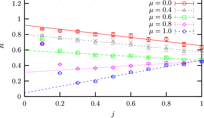
Figure 2: $R$ as a function of $j$ for various $\mu$.

Fig. 2 shows this extrapolated data plotted against $j$ for various values of $\mu$. One can immediately notice that although a linear fit through the data for $j\geq 0.3$ is reasonable, for $j<0.3$ the data departs sharply from the fit, especially in the high density phase $\mu$${\lower 2.0pt\hbox{$\scriptstyle>$}\atop\raise 4.0pt\hbox{$\scriptstyle\sim$}}$0.6. Possible origins of this effect are explored in section 4.4. Assuming that we can disregard the points with $j<0.3$, one can see from Fig. 2 that for $\mu=0$ a linear fit is consistent with a ratio of $R\approx 1$ corresponding to a manifest baryon number symmetry as one would expect in the vacuum. As $\mu$ is increased the value of the ratio decreases and as $\mu$ approaches one inverse lattice spacing we see that $R\approx 0$, suggesting that the ${\rm U}(1)_{B}$ symmetry is broken.

For more direct evidence of diquark condensation we study the diquark condensate defined in (14). Fig. 3 shows $\langle qq_{+}\rangle$ plotted against $j$ for various values of $\mu$. Again we have extrapolated linearly to the limit $L_{t}^{-1}\rightarrow 0$.

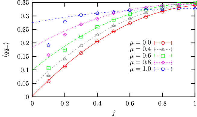
Figure 3: $\left<qq_{+}\right>$ as a function of $j$ for various $\mu$.

We use a quadratic fit through the data with $j\geq 0.3$ but again one can clearly see that for high $\mu$ the low $j$ points lie well below the curves. Ignoring these points we extrapolate to $j\rightarrow 0$. For $\mu=0$ we find no diquark condensation as expected, but as $\mu$ increases from zero, so does $\left<qq_{+}\right>$. We believe that the observations $\lim_{j\to 0}R=0$ and $\lim_{j\to 0}\langle qq_{+}\rangle\not=0$ together support the existence of a BCS phase at high chemical potential.

Finally, $\langle qq_{+}\rangle$ is plotted as a function of $\mu$ in Fig. 1. Although there is clearly a crossover from a phase with no diquark condensation to one in which the diquark condensate has a magnitude approximately that of the vacuum chiral condensate, this crossover is far less pronounced than in the chiral case. $\left<qq_{+}\right>$ increases approximately as $\mu^{2}$, (ie. as the surface area of the Fermi-sphere), but eventually saturates and even decreases as $\mu$ increases through 1. This may be a cut-off artifact. The curvature $\partial^{2}\left<qq_{+}\right>/\partial\mu^{2}$ is positive, in contrast to the behaviour observed in simulations of Two Colour QCD in which there is no Fermi surface and U(1)_B breaking proceeds via Bose-Einstein condensation [7]. It is possible, of course, that this behaviour for intermediate $\mu$ is an artifact of our poor control over the $j\to 0$ extrapolation.

4.3 The Low Temperature Lattice Fermi Surface

We know, from experience in 2+1$d$, that an extrapolation in $L_{t}^{-1}$ is the best description of of finite size corrections in this model. One natural progression would be to simulate with a small $L_{s}$ and various $L_{t}$, saving both CPU time and resources. However, this approach presents a problem.

As we increase $\mu$ we build up a Fermi surface, which in the continuum is a sphere smeared out by thermal fluctuations over a region $\delta k_{F}\sim 2T=(2L_{t})^{-1}$. In Euclidean space, an increase in $L_{t}$ corresponds directly to a decrease in temperature, and at low temperatures, the Fermi-Dirac distribution closely resembles a step-function with all states with $\sinh^{-1}\sqrt{\sum^{3}_{\nu=1}\sin^{2}k}\leq E_{F}$ occupied, and all other states unoccupied. If we simulate with $L_{t}\gg L_{s}$, the smearing of the Fermi surface will be too fine to be resolved on the coarse momentum lattice, and as $\mu\approx E_{F}$ is increased the physics will be constant except when the Fermi sphere crosses each momentum mode, turning any transition into a series of steps.

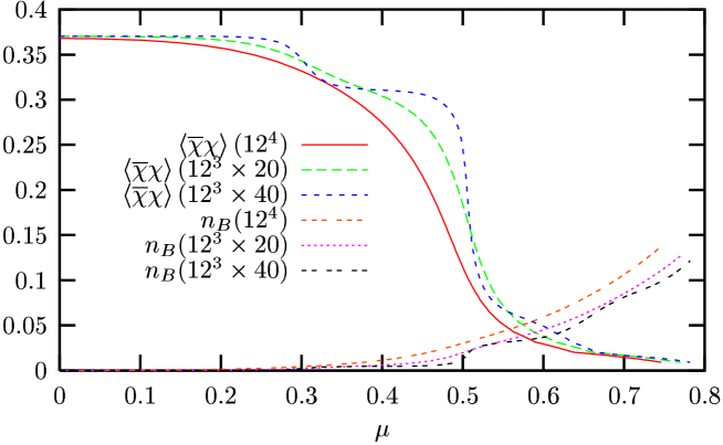
Figure 4: Chiral condensate and number density in the large-$N_{c}$ limit for various lattices.

Fig. 4 illustrates the effect that this has on the chiral transition in the large-$N_{c}$ limit. $\left<\overline{\chi}\chi\right>$ and $n_{B}$ are plotted on $12^{4}$, $12^{3}\times 20$ and $12^{3}\times 40$ lattices. On the asymmetric lattices one can clearly see the discontinuities caused as the Fermi surface crosses momentum modes. In the baryon number density one can even observe a plateau as the first mode becomes occupied. This behaviour was also observed in some initial lattice simulations. In practice, it seems that the effect is only prominent when $L_{t}$${\lower 2.0pt\hbox{$\scriptstyle>$}\atop\raise 4.0pt\hbox{$\scriptstyle\sim$}}$$3L_{s}/2$.

4.4 Finite Volume Effects

To investigate the possibility that the low-$j$ discrepancies in Figs. 2 & 3 are due to finite volume errors, it is necessary to study spatial volume dependence in a controlled manner. We study all $L_{s}^{3}\times L_{t}$ lattices with $L_{s}=6$, 8, 10, 12, 16 & 20 and $L_{t}=12$, 16 & 20 for fixed $\mu=1$. Being both well into the high-$\mu$ phase and far from the transition, any finite volume effects should be easily identifiable. We extrapolate to infinite temporal extent, corresponding physically to zero temperature, using the fact that the dominant finite size correction in our data is proportional to $L_{t}^{-1}$. However, Fig. 5 illustrates that there is some residual $L_{s}$ dependence.

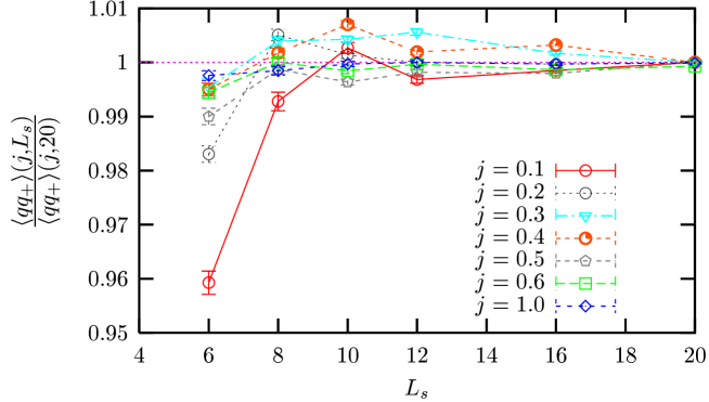
Figure 5: $\left<qq_{+}\right>$ in the zero-temperature limit as a function of the spatial extent of the lattice. The results are scaled such that $\left.\left<qq_{+}\right>\right|_{L_{s}=20}\equiv 1$.

$\left<qq_{+}\right>$ is plotted as a function of spatial extent for various values of $j$, with data presented as fractions of $\left.\left<qq_{+}\right>\right|_{L_{s}=20}$ to enable them to be displayed on the same axes. For $j\geq 0.5$, $L_{s}\geq 12$ the effect is negligible; the data are consistent within errors. For $j<0.5$ we observe non-monotonic fluctuations, whose magnitude increases with decreasing $j$. A possible explanation is that with a small source, the region about the Fermi surface in which diquark pairs would bind may be too fine to be resolved on small spatial lattices. Variational studies of the $N_{f}=2$, $N_{c}=3$ continuum NJL model at zero temperature in a finite spatial volume [14] find that with no diquark source, a spatial extent of 7fm ($\sim 35$ lattice spacings) is required before the model approximates its infinite volume limit. Below this volume, the BCS gap oscillates rapidly about its thermodynamic limit solution. Although this may explain why, with a small source, the condensate displays this non-monotonic $L_{s}$ dependence, for $L_{s}\geq 12$ these fluctuations are less than a $1\%$ effect, whereas the depletion of diquark pairs below the extrapolated curve in Fig. 3 is $\sim 30\%$. At this stage, therefore, we cannot claim to understand the origin of the depletion of diquarks at $j<0.3$.

5 Summary and Outlook

We have presented evidence for a BCS phase in the $3+1d$ lattice NJL model at high chemical potential, by measuring a diquark order parameter which appears, at $\mu=1$, to be of similar magnitude to the chiral order parameter in the vacuum. This is supported by a susceptibility ratio, $\lim_{j\to 0}R(\mu=1)\approx 0$, which suggests a broken ${\rm U}(1)_{B}$ baryon number symmetry in the high-$\mu$ phase. Both features contrast sharply with the equivalent measurements in the 2+1$d$ NJL model [11], where $\langle qq_{+}\rangle$ vanishes as a power of $j$ and $R$ is approximately a constant independent of $j$, both indicative of a critical phase with unbroken U(1)_B symmetry at high density.

Our measurement of $\langle qq_{+}\rangle$ can be translated into an order-of-magnitude estimate for the gap $\Delta$ using the following simple-minded argument: the condensate is the number density of bound diquark pairs, which in a BCS scenario is roughly equal to the volume of $k$-space within a distance $\Delta$ of the Fermi surface divided by the density of states; this yields $\langle qq_{+}\rangle\sim\Delta\mu^{2}$. Since at $\mu a=1.0$ we find $\langle qq_{+}\rangle a^{3}\sim m^{*}a\sim 0.2-0.3$, it is quite plausible that the gap values of ${\cal O}$(100MeV) predicted in [3] are possible.

Our claim to have observed a BCS phase in a lattice simulation is necessarily provisional, however, because it depends on the discarding of data with $j<0.3$, which in the high $\mu$ phase fall rapidly away from the trends observed at higher $j$. This threshold is very high when compared with chiral symmetry breaking at $\mu=0$, where the bare quark mass can be taken as low as $m_{0}=0.002$ with no adverse effects on $\langle\bar{\chi}\chi\rangle$ on the volumes studied. It is also larger by a factor of 3 than the equivalent threshold observed in 2+1$d$ [11]. The volume effects discussed in section 4.4 do not resemble those expected from the standard treatment of Goldstone fluctuations [15]. Variational studies in [14] suggest that with a vanishing source, a $7$fm spatial box ($L_{s}\sim 35a$), which is currently unattainable, may be required for the BCS state to approximate its infinite volume limit.

It is also possible that the low-$j$ discrepancy is a result of the partially quenched approximation, and would be resolved in a full unitary simulation. Although a repeat of the current study with a full simulation is currently beyond our reach, were it deemed necessary, it would be sufficient to repeat the study presented in section 4.4 with dynamical diquarks for a limited range of $j$. It should be noted, however, that no significant effect on diquark observables due to partial quenching was noted in [11].

We have chosen a value $m^{*}=350$MeV for the constituent quark mass in an attempt to simulate with phenomenologically reasonable parameters. The study of [14] was done with $m^{*}$ set to an equally reasonable 400MeV. Initial studies of the large-$N_{c}$ lattice model have determined that with this choice, the chiral transition changes character to become much sharper and may even become first order in the infinite volume limit. It is an interesting coincidence that this change in the order of the transition may occur in the “physical” region of parameter space. Not only is this worth exploring, but it might make the determination of a BCS phase more clear cut. It is also desirable to determine the lattice spacing $a$ by direct measurement of fermion and pion masses so that we can convert our results into physical units independent of the large-$N_{c}$ assumption. Finally, we wish to study the fermion dispersion relation, which will allow us to compare directly the chiral mass gap $\Sigma$ with the BCS gap $\Delta$, these being, in principle, physically measurable quantities.

References

-
[1]
K. Rajagopal and F. Wilczek,
in Handbook of QCD,
ch. 35, ed. M. Shifman (World Scientific, Singapore, 2001),
arXiv:hep-ph/0011333;
M.G. Alford, Ann. Rev. Nucl. Part. Sci. 51 (2001) 131. - [2] J. Bardeen, L.N. Cooper and J.R. Schrieffer, Phys. Rev. 108 (1957) 1175.
- [3] J. Berges and K. Rajagopal, Nucl. Phys. B538 (1999) 215.
- [4] M.G. Alford, J.A. Bowers and K. Rajagopal, Phys. Rev. D63 (2001) 074016.
- [5] J.B. Kogut, M.A. Stephanov, D. Toublan, J.J. Verbaarschot and A. Zhitnitsky, Nucl. Phys. B582 (2000) 477
- [6] S.J. Hands, I. Montvay, S.E. Morrison, M. Oevers, L. Scorzato and J. Skullerud, Eur. Phys. J. C17 (2000) 285.
-
[7]
R. Aloisio, V. Azcoiti, G. Di Carlo, A. Galante and A.F. Grillo,
Nucl. Phys. B606 (2001) 322;
J.B. Kogut, D.K. Sinclair, S.J. Hands and S.E. Morrison, Phys. Rev. D64 (2001) 094505;
S.J. Hands, I. Montvay, L. Scorzato and J. Skullerud, Eur. Phys. J. C22 (2001) 451. - [8] Y. Nambu and G. Jona-Lasinio, Phys. Rev. 122 (1961) 345; ibid 124 (1961) 246.
- [9] S.P. Klevansky, Rev. Mod. Phys. 64 (1992) 649.
- [10] S.J. Hands and S.E. Morrison, Phys. Rev. D59 (1999) 116002.
-
[11]
S.J. Hands, B. Lucini and S.E. Morrison,
Phys. Rev. Lett. 86 (2001) 753;
Phys. Rev. D65 (2002) 036004. - [12] S.J. Hands and J.B. Kogut, Nucl. Phys. B520 (1998) 382.
- [13] H. Kluberg-Stern, A. Morel, O. Napoly and B. Petersson, Nucl. Phys. B220 (1983) 447.
- [14] P. Amore, M.C. Birse, J.A. McGovern and N.R. Walet, Phys. Rev. D65 (2002) 074005.
- [15] P. Hasenfratz and H. Leutwyler, Nucl. Phys. B343 (1990) 241.