Kaon Weak Matrix Elements with Wilson Fermions

Abstract

We present results of several numerical studies with Wilson fermions relevant for kaon physics. We compute the $B_{K}$ parameter by using two different methods and extrapolate to the continuum limit. Our preliminary result is $B^{\overline{\mbox{\scriptsize MS}}}_{K}(2\mbox{ GeV})=0.66(7)$. $\Delta I=3/2$ $K\rightarrow\pi\pi$ matrix elements (MEs) are obtained by using the next-to-leading order (NLO) expressions derived in chiral perturbation theory (ChPT) in which the low energy constants (LECs) are determined by the lattice results computed at unphysical kinematics. From the simulation at $\beta\!\!=\!\!6.0$ our (preliminary) results read: $\langle\pi\pi|O_{7}^{\overline{\mbox{\scriptsize MS}}}(2\mbox{ GeV})|K\rangle_{I=2}\!\!=\!\!0.14(1)(1)\mbox{ GeV}^{3}$ and $\langle\pi\pi|O_{8}^{\overline{\mbox{\scriptsize MS}}}(2\mbox{ GeV})|K\rangle_{I=2}\!\!=\!\!0.69(6)(6)\mbox{ GeV}^{3}$.

1 $K^{0}$–$\bar{K}^{0}$ MIXING

The main problem of the computation of the $K^{0}$–$\bar{K}^{0}$ mixing amplitudes with Wilson fermions is the lattice operator mixing (not present in the continuum) introduced by the explicit breaking of the chiral symmetry due to the Wilson term. In order to compute the amplitudes one has to subtract contributions of operators with different naïve chiralities. Two alternative proposals which avoid the operator subtractions have been recently suggested: the first uses twisted mass QCD [1] while the second uses suitable Ward Identities (WIs) [2]. A first comparison of the standard method (with subtractions) to the WIs method (without subtractions) has been presented in ref. [3] for the case of the parameter $B_{K}$, defined as

$$\qquad\langle\bar{K}^{0}|O_{1}|K^{0}\rangle\equiv\frac{8}{3}f_{K}^{2}m_{K}^{2}B_{K},$$

with $O_{1}\!=\!Q_{1}\!-\!{\cal Q}_{1}\!=\!{\bar{s}}^{a}\gamma_{\mu}(1-\gamma_{5})d^{a}{\bar{s}}^{b}\gamma_{\mu}(1-\gamma_{5})d^{b}$. $Q_{1}$ is the parity conserving part of $O_{1}$ and under renormalization mixes with operators of different naïve chiralities, while ${\cal Q}_{1}$ is its parity violating part and due to ${\cal CPS}$ symmetry is multiplicatively renormalizable. The basic idea for the WIs method is based on the following WI obtained from a $\tau_{3}$ axial rotation:

$$m\sum_{z}\langle\Pi^{0}(z)P(t_{x},{\bf q}){\cal Q}_{1}(0)P(t_{y},{\bf q})\rangle+{\cal O}(a)=$$

$$\langle P(t_{x},{\bf q})Q_{1}(0)P(t_{y},{\bf p})\rangle+\textrm{(rot. sources),}$$

where $P(t,{\bf p})=\sum_{{\bf x}}e^{-i{\bf p}{\bf x}}\bar{d}(t,{\bf x})\gamma_{5}s(t,{\bf x})$ and $\Pi^{0}=\bar{d}\gamma_{5}d-\bar{u}\gamma_{5}u$. $SU(3)$ symmetry together with charge conjugation ${\cal C}$ imply that the terms involving the rotation of the sources are identically zero. Instead of computing the three point function involving $Q_{1}$ one can compute the four point function involving ${\cal Q}_{1}$, thus avoiding lattice operator mixing. From now on the procedure to obtain $B_{K}$ is common to both methods and can be found in ref. [4]. Note, however, that ${\cal O}(a)$ effects present in both methods may be different. Our simulation has been performed at three values of $\beta$, by keeping roughly the same physical volume.

$\beta$	6.0	6.2	6.4
volume	$16^{3}\times 52$	$24^{3}\times 64$	$32^{3}\times 70$
$\#$ confs.	500	200	135
$a^{-1}$ from $K/K^{*}$	2.05(7)	2.68(11)	3.44(10)
$aM_{P}$	0.30-0.39	0.20-0.35	0.15-0.23

The values of $B^{\overline{\mbox{\scriptsize MS}}}_{K}(2\mbox{ GeV})$ for each value of $\beta$ are given in Table 1, where the last column contains the values obtained from a linear extrapolation to the continuum limit (see Fig. 1). The average of the two gives $B^{\overline{\mbox{\scriptsize MS}}}_{K}(2\mbox{ GeV})=0.66(7)$. We are currently preparing a simulation at a larger $\beta$ to discard, eventually, the point at $\beta=6.0$ which could lie outside the region linear in $a$.

$\beta$	6.0	6.2	6.4	$\infty$
$a$ (fm)	0.096(3)	0.073(3)	0.057(2)	0
no subt.	0.818(32)	0.763(25)	0.750(37)	0.634(95)
stand.	0.890(45)	0.826(34)	0.819(40)	0.70(12)

Table 1. Values of $B^{\overline{\mbox{\scriptsize MS}}}_{K}(2\mbox{ GeV})$ in function of $a$

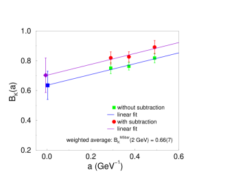
Figure 1: Continuum limit for $B^{\overline{\mbox{\scriptsize MS}}}_{K}(2\mbox{ GeV})$

2 $K\rightarrow\pi$ MEs IN THE CHIRAL LIMIT

The $K\!\!\rightarrow\!\!\pi$ MEs of $O^{3/2}_{7}$,$O^{3/2}_{8}$ (defined in ref. [6]) can be related, in the chiral limit, to those of the left-right operators of the $\Delta S\!\!=\!\!2$ basis as explained in ref. [6]. By using the soft pion theorem $\langle\pi\pi|O_{7,8}|K^{0}\rangle_{I=2}=-i/(\sqrt{2}f_{\pi})\langle\pi^{+}|O^{3/2}_{7,8}|K^{+}\rangle$, we obtain the $\Delta I\!\!=\!\!3/2$ MEs of the electro-weak penguin (EWP) operators $O_{7}$,$O_{8}$ (defined in Eq. (1) of ref. [5]) in the chiral limit. Our results (in the $\overline{\mbox{\scriptsize MS}}$ scheme at $2\mbox{ GeV}$) read:

$\beta$	6.0	6.2	6.4
$\!\!\!\!\langle\pi\pi|O_{7}|K^{0}\rangle_{I=2}[\!\!\mbox{ GeV}^{3}\!]$	0.132(10)	0.136(14)	0.136(10)
$\!\!\!\!\langle\pi\pi|O_{8}|K^{0}\rangle_{I=2}[\!\!\mbox{ GeV}^{3}\!]$	0.658(44)	0.604(44)	0.533(34)

For $O_{8}$ discretization errors seem quite large and we are currently investigating this feature.

3 $\Delta I=3/2$ $K\rightarrow\pi\pi$ AMPLITUDES

The procedure to extract these amplitudes by using ChPT at NLO has been explained in ref. [5, 7, 8]. We are interested in $K\rightarrow\pi\pi$ matrix elements of the EWPs and of the operator $O_{4}$ (defined in Eq. (1) of ref. [5]) which mainly determines the physical $K^{+}\rightarrow\pi^{+}\pi^{0}$ decay amplitude. In practice we work with an unphysical kinematics (called SPQR) where the kaon is at rest, one pion is at rest and the other has either momentum 0 or momentum $2\pi/L$. We have 3 pion masses and 3 kaon masses for each pion one ($M_{\pi}\in[0.51,0.88]\mbox{ GeV},\,M_{K}\in[0.51,1.46]\mbox{ GeV}$), and the energy is in general not conserved (it can be injected through the weak operator [9]). We fit the numerical data to the expressions obtained at NLO in quenched ChPT [5, 8]. For example, for the EWPs we have $\displaystyle{\cal M}_{7,8}^{\textrm{\tiny{SPQR}}}\!\!\!\!$ $\displaystyle=\gamma^{7,8}\left(1+\frac{M_{K}^{2}}{(4\pi f)^{2}}(\textrm{chiral logs})^{\textrm{\tiny{SPQR}}}\right)$ $\displaystyle-\left(\delta^{7,8}_{3}+\frac{\delta^{7,8}_{2}}{2}-\frac{\delta^{7,8}_{1}}{2}\right)\,M_{K}\,(M_{\pi}+E_{\pi})$ $\displaystyle+\left(\delta^{7,8}_{4}+\delta^{7,8}_{5}\right)\left(2M^{2}_{K}+4M^{2}_{\pi}\right)$ $\displaystyle+\delta^{7,8}_{6}\left(4M^{2}_{K}+2M^{2}_{\pi}\right)-(\delta^{7,8}_{1}+\delta^{7,8}_{2})\,E_{\pi}\,M_{\pi},\;\qquad\quad(1)$

Figure 2: Numerical data for the ME of $O_{8}$

where $\gamma^{7,8}$ is the LEC of the LO while the $\delta^{7,8}_{i}$ are the LECs of the NLO. For the moment we have not considered the finite volume correction (the Lellouch-Lüscher (LL) factor [10]) which is not yet known for the SPQR kinematics. In this way we determine some combinations of the LECs of the NLO and we use them to compute the values of the physical amplitudes (see refs. [5, 8] and refs. therein). Again in the case of the EWPs we have

$${\cal M}^{\tiny{\textrm{phys}}}_{7,8}\!\!\!\! =\gamma^{7,8}\left(1+\frac{m_{K}^{2}}{(4\pi f)^{2}}(\textrm{chiral logs})^{\textrm{\tiny{phys}}}\right)$$

$$+\left(-\delta^{7,8}_{2}-\delta^{7,8}_{3}+2\delta^{7,8}_{4}+2\delta^{7,8}_{5}+4\delta^{7,8}_{6}\right)\,m^{2}_{K}$$

$$+\left(\delta^{7,8}_{1}+\delta^{7,8}_{2}+4\delta^{7,8}_{4}+4\delta^{7,8}_{5}+2\delta^{7,8}_{6}\right)\,m^{2}_{\pi}.$$

For the EWPs, 6 counterterms of the NLO contribute in the SPQR kinematics and, as shown in Eq. (1), we can determine only 4 combinations of the corresponding LECs. These are enough to compute the physical amplitude. For $O_{4}$ there are again 6 counterterms at the NLO but all of the corresponding LECs have to be separately determined. Consequently, in the second case the fit is much more complicate.

For the EWPs, the analysis at LO (which is ${\cal O}(p^{0})$ and thus correspond to fit the numerical data to a constant) gives the results

$M_{K},E_{\pi}<$	1.5 GeV	1.0 GeV	0.8 GeV
$\langle\pi\pi|O_{7}|K^{0}\rangle_{I=2}$	0.076(6)	0.080(6)	0.094(6)
$\langle\pi\pi|O_{8}|K^{0}\rangle_{I=2}$	0.909(45)	0.860(45)	0.803(46)

where we varied the number of data points used in the fit by choosing only points with masses and energies below a certain cut-off. The dependence of the results on the cut-off is due to the fact that higher orders in ChPT are not negligible (as one can argue from Fig. 2 in the case of $O_{8}$). We thus introduce the NLO ${\cal O}(p^{2})$ contribution in the fit. In Fig. 3 we show the quality of the fits obtained by using either the logarithms of full ChPT or those of quenched ChPT.

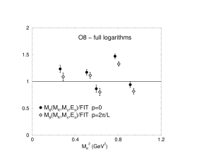
Figure 3: Fits to ${\cal M}_{8}$ with full and quenched logs

We see that, according to what expected [11], only the quenched logarithms have the appropriate form to fit the data. On the other hand, the fit is not very sensitive to the quenching parameters $\delta$ and $\alpha$ [12] and, in the lacking of their precise determination, we set their values to be $\delta=0.1$ and $\alpha=0.0$. The contributions of the LO and NLO to the fit are shown in Fig. 4. The fit now shows much less dependence on the cut-off and we quote the results obtained with $M_{K},E_{\pi}<0.8$ GeV as our central values, and use those with other cut-offs to estimate the systematic error due to the higher-order corrections in the chiral expansion. This leads to the preliminary results (in which the finite-volume LL corrections have not been included):

$$\langle\pi\pi|O_{7}^{\overline{\mbox{\scriptsize MS}}}(2\mbox{ GeV})|K\rangle_{I=2}=0.14(1)(1)\mbox{ GeV}^{3},$$

$$\langle\pi\pi|O_{8}^{\overline{\mbox{\scriptsize MS}}}(2\mbox{ GeV})|K\rangle_{I=2}=0.69(6)(6)\mbox{ GeV}^{3}. \;(2)$$

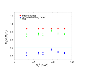
Figure 4: Various contributions to the fit of ${\cal M}_{8}$

Note, however, that we can not claim to be sensitive to the chiral logarithms. In fact we could have fitted our numerical data by including only the counterterms of the NLO and not the logarithms. Also in this case we would have obtained a very good fit (of quality comparable to that which includes the chiral logarithms) and results which depend very weakly on the cut-off and which are very close to those obtained by including the logarithms: $\langle O_{7}\rangle_{I=2}\!\!=\!\!0.13(1)(1)\mbox{ GeV}^{3}$ and $\langle O_{8}\rangle_{I=2}\!\!=\!\!0.64(6)(2)\mbox{ GeV}^{3}$. We also note that this determination and the one in Eq. (2) are both in reasonable agreement with the results obtained from $K\!\!\!\rightarrow\!\!\pi$ MEs in Sec.2 (at $\beta\!\!=\!\!6.0$). Finally, it is important to remark that the analysis at LO would lead to a large systematic error (as large as $40\%$ in the case of $O_{7}$).

Also in the case of $O_{4}$ the NLO contribution turns out to be large. The fit is more problematic due to the large number of parameters and the errors on some of the NLO LECs (and therefore on the whole NLO contribution) is quite large. As an indicative result (obtained with $M_{K},E_{\pi}<1\mbox{ GeV}$) we quote ${\cal A}(K^{+}\!\!\!\rightarrow\!\!\!\pi^{+}\pi^{0})\!\!\!=\!\!\!0.0097(18)^{LO}\!\!\!+\!\!\!0.0039(85)^{NLO}\mbox{ GeV}^{3}$ (the experimental value is ${\cal A}^{\tiny{\textrm{exp}}}\!\!\!=\!\!\!0.0104\mbox{ GeV}^{3}$). We are presently trying to consider other kinematical configurations which could improve the quality of the fit.

References

• [1] M. Guagnelli et al., [hep-lat/0110097].
• [2] D. Becirevic et al., [hep-lat/0005013].
• [3] D. Becirevic et al., [hep-lat/0110006].
• [4] L. Conti et al., [hep-lat/9711053].
• [5] Ph. Boucaud et al., [hep-lat/0110206].
• [6] A. Donini et al., [hep-lat/9910017].
• [7] Ph. Boucaud et al., [hep-lat/0110169].
• [8] C.-J.D. Lin et al., [hep-lat/0208007].
• [9] C.-J. D. Lin et al., [hep-lat/0104006].
• [10] L. Lellouch and M. Lüscher, [hep-lat/0003023].
• [11] C.-J.D. Lin et al., [hep-lat/0209020].
• [12] C. Bernard et al., [hep-lat/9204007].