Abstract

We present recent results in unquenched lattice QCD with two degenerate light sea quarks using the truncated determinant approximation (TDA). In the TDA the infrared modes contributing to the quark determinant are computed exactly up to some cutoff in quark off-shellness (typically 2$\Lambda_{QCD}$). This approach allows simulations to be performed at much lighter quark masses than possible with conventional hybrid MonteCarlo techniques. Results for the static energy and topological charge distributions are presented using a large ensemble generated on very coarse (6⁴) but physically large lattices. Preliminary results are also reported for the static energy and meson spectrum on 10³x20 lattices (lattice scale $a^{-1}$=1.15 GeV) at quark masses corresponding to pions of mass $\leq$ 200 MeV. Using multiboson simulation to compute the ultraviolet part of the quark determinant the TDA approach becomes an exact algorithm with essentially no increase in computational effort. Some preliminary results using this fully unquenched algorithm are presented.

1 Introduction

Although much progress has been made in the last few years towards the goal of simulating important hadronic quantities in fully unquenched lattice QCD, the physical regime of light up and down sea quarks (quark masses $<$10 MeV) remains basically intractable with the current standard algorithms (hybrid MonteCarlo (HMC) and variants thereof [1]) even with the Teraflop scale parallel platforms which are presently coming online. With these algorithms, the generation of a statistically significant ensemble of dynamical gauge configurations with “light” quark masses chosen to give a pion mass just light enough to allow rho decay (on sufficiently large lattices) already consumes many Teraflop years of computational effort [2]. The high cost of performing unquenched HMC simulations with light sea quarks arises from two independent sources: the sensitivity of conjugate gradient solvers of large systems to the condition number of the matrix to be inverted, and the growing autocorrelation time due to critical slowing down as the critical point corresponding to the chiral limit at which the pseudoscalar mass vanishes is approached. Most of the power growth (as a function of inverse pion mass) in the computational effort is in fact due to the first of these sources [2], which the algorithms described in this paper are designed to circumvent.

Let us first recall the origin of the problems with the iterative solvers used in typical HMC simulations of unquenched QCD. To be specific, we consider throughout the case of Wilson (or Sheikoleslami-Wohlert “clover” improved) quark actions. The desired quark determinant (with two degenerate flavors of sea quark) is introduced via pseudofermionic fields with a quadratic action involving the inverse of the squared quark (Wilson/clover)-Dirac operator $Q$. The system is then treated as a classical Hamiltonian one subjected to molecular dynamics evolution corresponding to the following Hamiltonian

$$\cal{H}_{MD} = \frac{1}{2}\rm{Tr}(P_{U}^{2})+S_{\rm gauge}(U)+\phi^{\dagger}(Q^{\dagger}Q)^{-1}\phi$$ (1)

$$Q^{\dagger}Q = H^{2},\;\;\;\;H\equiv\gamma_{5}Q\;\;\;(\rm{hermitian})$$ (2)

where $P_{U}$ are the conjugate momenta to the gauge-fields $U$, $S_{\rm gauge}(U)$ is the pure gauge action, and $\phi$ is a bosonic field with a highly nonlocal action. In order to update the gauge-fields, the force on these fields due to the $\phi$ field must be computed, and this involves the inversion of the $Q^{\dagger}Q$ operator, which is identical to the square of the hermitian Wilson-Dirac operator $H\equiv\gamma_{5}Q$. As the quark mass is taken to zero, the operator $H$ frequently develops very small eigenvalues: equivalently, the condition number (ratio of highest to lowest eigenvalue) not uncommonly becomes very large (in simulations described later in this paper, condition numbers $>$1000 are quite common for $H$). The required inversion of $H^{2}$ in Eq(1) then involves an operator of condition number $>$10⁶, which not surprisingly requires a very large number of conjugate gradient sweeps. In a nutshell, most of the computational difficulty with very light sea-quarks in the standard hybrid MonteCarlo algorithm arises from this source.

In contrast to the “freezing” problem encountered with linear solvers of the conjugate gradient variety, the extraction of low eigenvalues by Krylov subspace methods such as the Lanczos algorithm [3] does not deteriorate as a consequence of the presence of a very small eigenvalue. The rapidity with which the Lanczos procedure extracts eigenvalues in a given region of the spectrum is instead determined by the local spectral density in that region, which for the operator $H$ of interest to us here is in fact minimal near zero. The eigenvalues of $H$ (cf. Section 2) have the physical interpretation as a gauge-invariant extension of quark off-shellness in the free theory, so the truncation of the full quark determinant to a product of all modes with (absolute value) eigenvalue below some cutoff $\mu$ corresponds to a gauge-invariant approximation of the fully unquenched theory in which sea-quark loops up to quark off-shellness $\mu$ are included exactly and completely. This approximation will be referred to as the “truncated determinant approximation” (TDA) in the following. In previous publications various features of the implementation of this algorithm have been discussed [4, 5], as well as the application to the study of stringbreaking on large coarse lattices [6]. The work described here is motivated to a large extent by a desire to provide alternatives to HMC which would allow at least some quantities to be computed directly in the deep chiral regime as a check on the large extrapolations required from the quark masses presently practicable in the HMC approach to the physical range.

In Section 2, we review the basic features of a truncated determinant approach to unquenched QCD in the light of the much more extensive simulations which we have performed since the aforementioned references. In particular, we argue that many low-energy hadronic quantities (e.g. low-lying hadron spectrum, string-breaking, low energy chiral physics) can be studied quite precisely in the TDA approximation, while other effects which depend more sensitively on the ultraviolet structure of internal quark loops (e.g. channels involving the eta-prime) require a fully consistent treatment of the full quark determinant. In Section 3 we present recent results obtained with large ensembles ($\simeq$10000 configurations) of unquenched TDA configurations on physically large, coarse lattices ($6^{4}$, with O($a^{2}$) gauge action improvement): the quantities studied include the static energy of a heavy quark-antiquark pair, and dependence of topological charge distributions on the quark mass. In Section 4 we present some preliminary results obtained on larger lattices (10³x20, with a lattice scale $a^{-1}$=1.15 GeV): here we concentrate on extracting the low-lying meson spectrum at up and down sea-quark masses close to their physical values ($m_{\pi}/m_{\rho}<0.26$). We also give an example of a correlator in which the truncated determinant approximation introduces a visible anomaly analogous (but quantitatively less severe) to the one familiar from quenched calculations: namely, the scalar isovector channel [10]. Finally, in Section 5, we describe a combined TDA + multiboson approach which allows exact unquenched simulations in the very light quark regime with a small number of multiboson fields. Some preliminary results of simulations on large coarse lattices with this technique are described.

2 Infrared and Ultraviolet Quark Modes: the Truncated Determinant Approximation

The hermitian (Euclidean) Dirac operator $H\equiv\gamma_{5}(D\!\!\!\!/(A)-m)$ has a spectrum which can be regarded as the gauge-invariant generalization to nontrivial gauge fields of the quark off-shellness of the free quark theory. Indeed, the eigenvalues of the free operator $H_{0}\equiv\gamma_{5}(D\!\!\!\!/(A=0)-m)$ are just $\pm\sqrt{p^{2}+m^{2}}$, which precisely corresponds to the signed Euclidean off-shellness of a quark of mass $m$ and momentum $p$. Moreover, the individual eigenvalues (though not, of course, the eigenvectors) are gauge-invariant. Roughly speaking, we can therefore visualize the contribution to the quark determinant from the infrared modes (corresponding to the eigenvalues of $H$ of smallest absolute value) as arising from quark loops of large physical extension in Euclidean coordinate space, while the ultraviolet modes correspond to quark loops of small size. Gauge-invariant quark loops of small size correspond to the lowest dimension gauge-invariant operators so we should expect that the contribution to the quark determinant from the highest UV modes amounts to a functional of exactly the same form (i.e. $\int F_{\mu\nu}^{2}d^{4}x$ in the continuum) as the basic pure gauge action, and therefore has the sole physical effect of changing the scale in any gauge-invariantly cutoff version of the theory, such as lattice QCD.

To make these arguments a little more concrete, let us imagine separating low and high quark eigenmodes in an analytically smooth way by switching off the higher eigenvalues above a sliding scale $\mu$. If we define

$$D(\mu)\equiv\frac{1}{2}\rm{tr\;ln}(\tanh{\frac{H^{2}}{\mu^{2}}})$$ (3)

then a weak-coupling expansion of $D(\mu)$ shows [4] that the $\mu$ dependence is given asymptotically for large $\mu$ by

$$D(\mu)\simeq\beta_{F}\ln{\frac{\mu^{2}}{m_{q}^{2}}}\int d^{4}xF_{\mu\nu}^{2}+O(\frac{1}{\mu^{2}}(DF)^{2})$$ (4)

where $\beta_{F}$ is the one-loop quark contribution to the beta function. This result illustrates in an explicit way the role of the high quark modes in renormalizing the pure gauge action, which physically corresponds to the screening of the gauge interactions by virtual quark-antiquark pairs.

The above considerations suggest in the case of lattice QCD a natural (and gauge-invariant) truncation of the full theory in which the quark determinant is split into an infrared and ultraviolet part at an appropriately chosen scale $\mu$. In the lattice case, the operator $H$ is a large, sparse hermitian matrix with eigenvalues $\lambda_{i}$, and we may write

$$\rm{det}(H^{2})=(\prod_{|\lambda_{i}|<\mu}\lambda_{i}^{2})(\prod_{|\lambda_{i}|>\mu}\lambda_{i}^{2})\equiv D_{IR}(\mu)\cdot D_{UV}(\mu)$$ (5)

for the quark determinant appropriate for two degenerate sea-quark flavors. For sufficiently high $\mu$, the contribution of $D_{UV}$ to the effective action (after integrating out quark fields) should amount to a renormalization of the pure gauge action. Specifically, we expect that $D_{UV}$ should be accurately modelled by small Wilson loops which can then be absorbed into the pure gauge part of the action and should induce, at least for low energy quantities dominated by processes in which virtual quark off-shellness is typically lower than $\mu$, only a change of lattice scale, while leaving dimensionless quantities (such as ratios of hadron masses) unchanged. This expectation has been confirmed by extensive numerical studies [5], which show that in many cases $D_{UV}$ is accurately modelled by linear combinations of loop operators containing 6 links or less. In these studies, it was important to perform the IR-UV split by choosing a fixed number $N_{\rm eig}$ of low eigenvalues: $\mu$ is then the average value of $|\lambda_{N_{\rm eig}}|$ (where the eigenvalues of $H$ are always ordered with respect to absolute magnitude). Otherwise, a small variation of the gauge configuration can cause $|\lambda_{N_{\rm eig}}|$ to cross the scale $\mu$, resulting in a discontinuous jump in $D_{UV}$, a situation clearly incompatible with a smooth analytical fit of $D_{UV}$ to a fixed linear combination of small Wilson loops. Accordingly, for the rest of this paper, we shall define

$$D_{IR}(\mu) \equiv \ln{\prod_{i=1}^{i=N_{\rm eig}}\lambda_{i}^{2}}$$ (6)

$$D_{UV}(\mu) \equiv \ln{\prod_{i=N_{\rm eig}+1}\lambda_{i}^{2}}$$ (7)

$$\mu \equiv <|\lambda_{N_{\rm eig}}|>$$ (8)

The truncated determinant approximation (TDA) will correspond to the interpolation between quenched and full QCD induced by replacing the full quark determinant by the infrared piece $D_{IR}$ in the effective pure gauge action obtaining after quark fields are integrated out. We shall argue below that a choice of truncation scale $\mu\simeq 2\Lambda_{QCD}$ is adequate to preserve both the important low energy chiral physics of QCD, as well as the low-lying hadron spectrum (lowest states in each channel). Moreover, the computational difficulty of extracting the (typically, several hundred) eigenvalues needed for $D_{IR}$ does not increase as the quark mass is taken to zero on a fixed size lattice, in contrast to conventional HMC algorithms.

3 TDA simulations on large, coarse lattices

The TDA approach has been applied previously to a study of stringbreaking in physically large (2.4 fermi⁴) lattices at a single value of the sea-quark mass [6]. These simulations have been extended to four different sea-quark masses (with 2 degenerate flavors of sea-quark) with ensembles 2-2.5 times larger than previously studied. In order to study long distance features of the full theory, we work on coarse 6⁴ lattices (lattice spacing $a=$0.4 F) but with O($a^{2}$) improved gauge action. Following Alford et al [7], we improve the gauge action with a single additional operator, with coefficients tuned to optimize rotational invariance of the string tension

$$S(U) = \beta_{\rm plaq}\sum_{\rm plaq}\frac{1}{3}{\rm ReTr}(1-U_{\rm plaq})$$ (9)

$$+ \beta_{\rm trt}\sum_{\rm trt}\frac{1}{3}{\rm ReTr}(1-U_{\rm trt})$$

where “trt” refers to a 8 link loop of generic structure (+x,+y,+x,-y,-x,+y,-x,-y) (the “twisted rectangle” of Ref[7]). With the choices $\beta_{\rm plaq}$=3.7, $\beta_{\rm trt}$=1.04$\beta_{\rm plaq}$, the violations of rotational invariance expected on such a coarse lattice are almost completely eliminated so that the static quark potential becomes a smooth function of lattice radial separation [7]. As the quark action is not improved, the lattice spacing quoted here is determined by matching the initial linear rise of the string tension to a physical value (rather than by using the rho mass, for example).

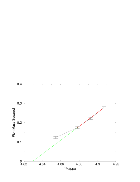
Figure 1: Fit of $M_{\pi}^{2}$ versus $1/\kappa$

All four values for the sea-quark hopping parameter studied here correspond to very light quarks by the usual standards of unquenched QCD. In Fig. 1 we show the plot of pion mass squared versus $\frac{1}{\kappa}$. The lightest quark shows a clear finite volume effect in the pion mass, so we have determined the critical kappa value from a fit to the heaviest three quarks only, as indicated in the figure. This fit gives $\kappa_{c}=$0.20706. In physical units, the three heaviest quarks correspond to pion masses of 210, 235 and 264 MeV, while the lightest sea-quark studied corresponds to a pion mass of 175 MeV in the finite volume system, or an infinite volume pion mass of about 150 MeV, very close to the physical value.

Figure 2: Monte Carlo sequence of $D_{IR}$ for $\kappa$=0.2050

Figure 3: Autocorrelation curve of $D_{IR}$ for $\kappa$=0.2060

In the TDA simulations described here the number of infrared modes included exactly in the low-energy determinant $D_{IR}$ has been chosen to be 840, for all four kappa values. The lattice scale as determined from the initial linear rise of the static energy is essentially unchanged over the limited range of quark masses studied and so is the magnitude of the largest included eigenvalue of $H$ (in lattice units: see Table 1), so the scale $\mu$ for the determinant truncation corresponds in all cases to a physical off-shellness of approximately $410$ MeV. The global gauge-field update which precedes the accept/reject step based on the change in $D_{IR}$ is a standard multihit metropolis [6], with parameters chosen to ensure an acceptance ratio on the order of 50% (see Table 1). These parameters are the same for all four runs, but the acceptance ratio varies only from 49% to 58% even though the quark mass varies by a factor of 3.

In Table 1, we also show the results of autocorrelation studies of the infrared determinant $D_{IR}$, and of the topological charge. The sequence of infrared determinant $D_{IR}$ values shows the existence of very long correlations in this quantity, as is apparent in Fig. 2, typically extending over thousands of update steps (1 update step $\equiv$ 1 global gauge-field update followed by an accept/reject based on $D_{IR}$). This makes it difficult to extract an accurate autocorrelation time, even with a sequence of 100000 steps. The determinant autocorrelation times $\tau_{\rm det}$ shown in Table 1 are obtained by integrating the autocorrelation curves out to a Monte Carlo time where they first cross zero, but these curves are not even approximately exponential (see Fig. 3), so there are undoubtedly several important time scales present in the MonteCarlo dynamics for this quantity.

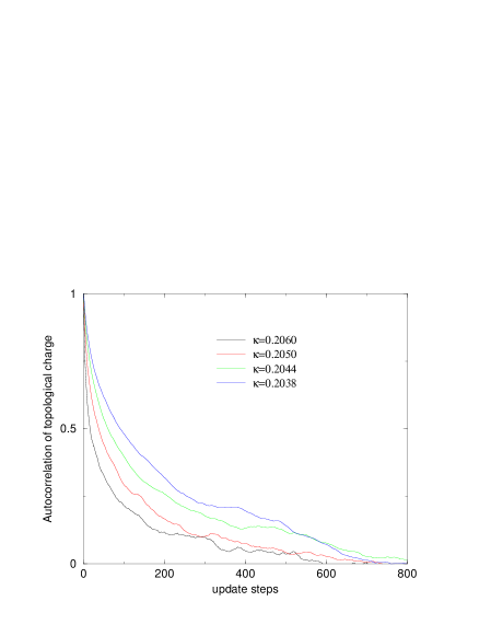
Figure 4: Autocorrelation curves of $Q$ for $\kappa$=0.2060,0.2050,0.2044,0.2038

For the topological charge, the situation is much cleaner. The topological charge, $Q$, can be expressed [4] in terms of the eigenvalues of the Wilson-Dirac operator:

$$Q={1\over 2\kappa}(1-{\kappa\over\kappa_{c}})\sum_{i=1}^{N}{1\over\lambda_{i}}$$

In practice, this sum is quickly saturated by the low eigenvalues: in particular, we have evaluated it by setting $N=N_{\rm eig}$, as these eigenvalues are in any case byproducts of the TDA update procedure. The autocorrelation curves for $Q$ for the 4 different $\kappa$ values are shown in Fig. 4 and are roughly exponential: the autocorrelation times $\tau_{\rm top}$ given by the integral of the autocorrelation function are displayed in Table 1. For the lighter quarks, the autocorrelation time determined by an exponential fit at small times is somewhat smaller, indicating the presence of a longer range component.

Table 1: Characteristics of 4 6⁴ TDA ensembles, a=0.4 F

Run	$\kappa$	$M_{\pi}$	$F_{\pi}$	$<|\lambda_{N_{\rm eig}}|>$	accpt. ratio	$\tau_{\rm det}$	$\tau_{\rm top}$
j1	0.2060	0.351 $\pm$ 0.008	0.19	0.826	0.49	$\simeq$2.9x103	75
j2	0.2050	0.418 $\pm$ 0.006	0.21	0.828	0.51	$\simeq$1.4x103	105
j3	0.2044	0.472 $\pm$ 0.006	0.20	0.827	0.57	$\simeq$3.5x103	157
j4	0.2038	0.528 $\pm$ 0.006	0.18	0.827	0.57	$\simeq$2.3x103	182

The static energy of a heavy quark-antiquark pair has been studied for the four ensembles described above. Coulomb gauge Wilson lines [6] were accumulated after every update step until a bin size of 2000 steps was reached. The corresponding binned Wilson line averages (typically, on the order of 40 to 50) were then subjected to a standard bootstrap analysis, allowing us to extract asymmetric errors. Also, the bin size was varied until the errors were stable to ensure that autocorrelation effects were eliminated. For the lightest two quark masses (runs j1,j2) there is reasonably clear evidence of stringbreaking once the Wilson line ratios are taken between Euclidean times 1.2 fm and 1.6 fm (T=3/4 plots on Figs. 5,6, with the large R value agreeing with (twice) the measured mass for a heavy-light meson. With the heaviest mass sea-quark the levelling off of the static energy at larger distance is less clear (Fig. 7). Even with the large ensembles collected, it is clear that the sea-quark shielding of the string tension induces very large fluctuations which makes high precision very hard to achieve.

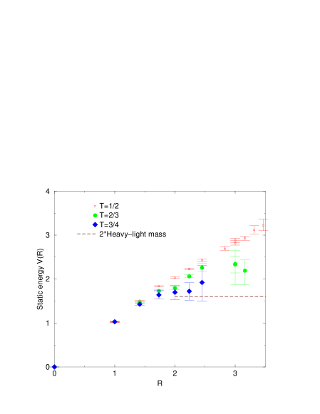
Figure 5: Static Energy $V(R)$ for $\kappa$=0.2060 (j1 run)

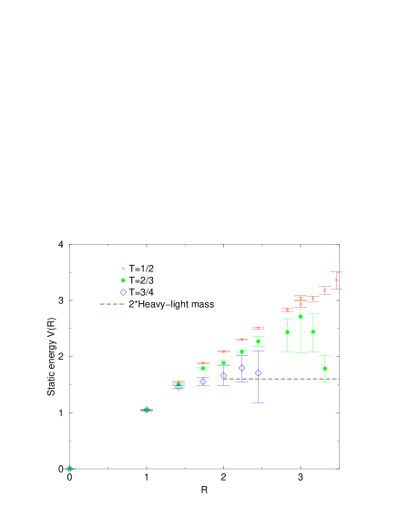
Figure 6: Static Energy $V(R)$ for $\kappa$=0.2050 (j2 run)

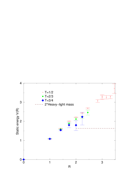
Figure 7: Static Energy $V(R)$ for $\kappa$=0.2038 (j4 run)

Another very characteristic feature of unquenched QCD in the chiral limit arises from the suppression of nontrivial topological charge as the quark mass goes to zero. The distribution of topological charge $Q$ is known [9] to follow directly from the chiral symmetry of QCD. In the case of a theory with two degenerate light quark flavors, the normalized probability distribution of $Q$ in a system of finite space-time volume $V$ is given by

$$P(Q) = x\frac{I_{Q}(x)^{2}-I_{Q+1}(x)I_{Q-1}(x)}{I_{1}(2x)}$$

$$x \equiv \frac{1}{2}Vf_{\pi}^{2}M_{\pi}^{2}$$ (10)

An accurate determination of $f_{\pi}$ in the usual fashion from pseudoscalar-axial vector correlators is difficult on such small lattices, as the only time window available is T=1-2 (the axial correlator is antiperiodic and vanishes at T=3). However, it is apparent from (3) that $f_{\pi}$ can be extracted from the topological charge distribution by a one-parameter fit of the dimensionless $x$ variable, once the pion masses have been measured. In Fig. 8 we show the measured distributions (diamonds) of $Q$ for the four different sea-quark values as well as the fits to the chiral prediction (3). The narrowing of the distribution as one goes to lighter quarks is clearly visible. The values of $f_{\pi}$ extracted from the fit $x$ values are given in Table 1. At $\kappa=$0.2050 the value of $f_{\pi}$ has been previously extracted from a large ensemble study of axial vector correlators using all-point quark propagators [8]: this method gives $f_{\pi}=$0.187$\pm$0.011, close to the value 0.21 found from the topological charge fit. Also, the value of $f_{\pi}$ is fairly constant over the (limited) range of sea-quark masses studied, as we expect. These results certainly contribute to our confidence that the TDA method builds in all the important low energy chiral physics of QCD.

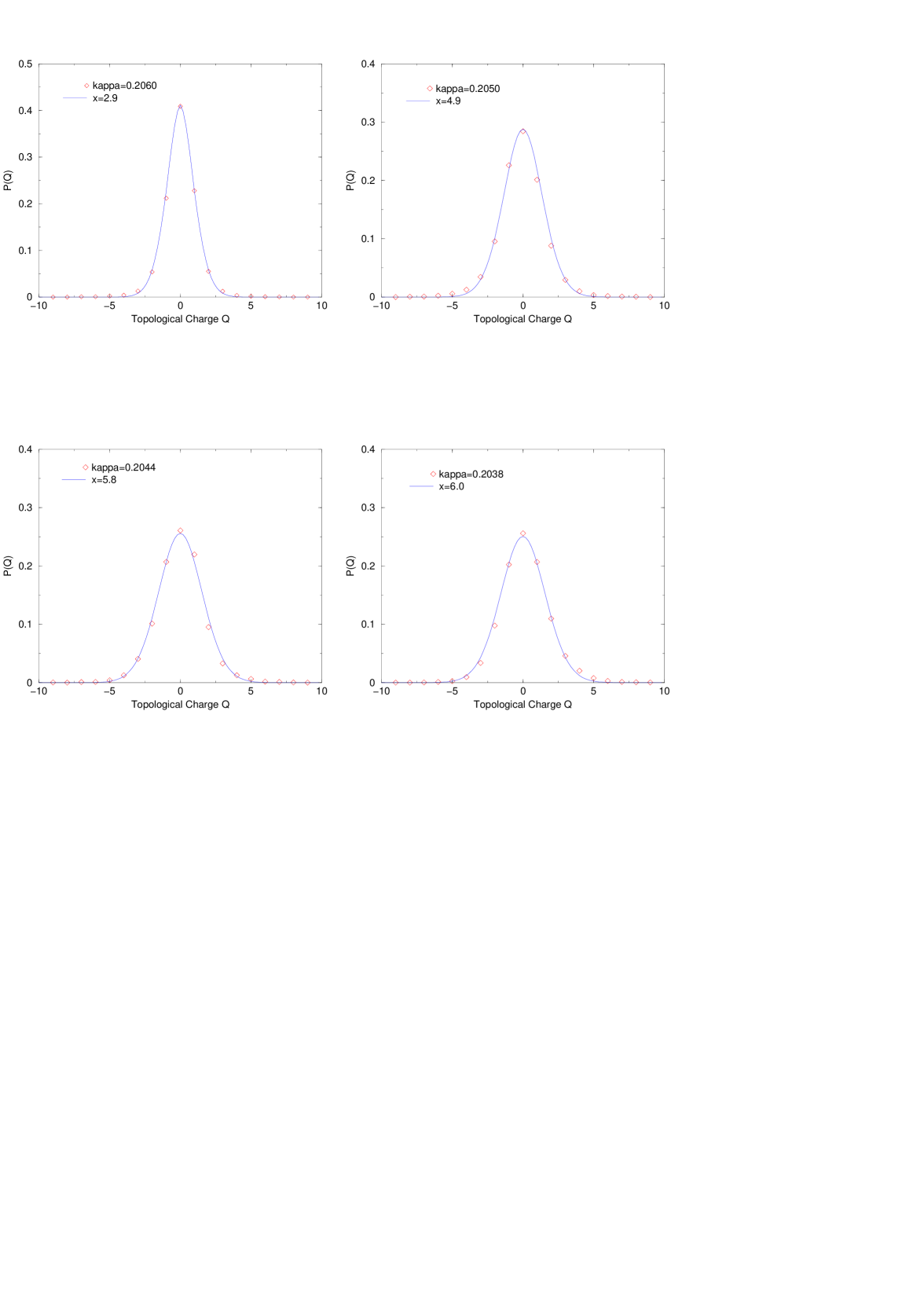
Figure 8: Topological charge distributions and fits for $\kappa=$0.2060,0.2050,0.2044,0.2038

4 TDA simulations on finer lattices

Although unquenched simulations on physically large but coarse lattices may yield useful qualitative insights (especially with regard to the dynamics of the simulation process), we can only expect quantitatively useful results by simulating larger and finer lattices. A number of TDA simulations on 10³x20 lattices at a lattice spacing $a^{-1}$=1.15 GeV have therefore been performed to assess the practicality of the TDA method for larger lattices (the increase in computational effort required for even larger lattices is discussed at the end of this section). The gauge action used in this case is a single plaquette one as improvement is not as important with a lattice spacing of order 0.17 fermi as it was in the case of the coarse lattices with spacing 0.4 fermi discussed in the preceding section. However, we have used clover improvement (with a Sheikoleslami-Wohlert coefficient of $C_{sw}=$1.57) for the fermions. This allows us to determine the lattice spacing from the rho mass, rather than the string tension, although the two values are basically quite consistent, as we discuss below. In the TDA simulations, the lowest 520 eigenvalues were kept, corresponding to a TDA scale of about 504 MeV. The Lanczos extraction of these eigenvalues for a single configuration takes about 1.3 hours on a Pentium-4 1.7GHz processor: as this completely dominates the computational effort, this time also represents a single update step of the TDA simulation for these lattices.

The preliminary results described in this section were obtained from two separate ensembles corresponding to runs at $\beta=$5.7 and $\kappa=$0.1420 (h1 run) and 0.1415 (h2 run). To this point, 100 configurations separated by 50 update steps were obtained for the h2 run and 80 configurations for the lighter h1 run. Most of the discussion will concern the h2 run as finite volume effects, available statistics and autocorrelation effects are all worse for the h1 run. The simulations are continuing and we expect to accumulate significantly larger ensembles in the coming months, by implementing a completely parallel version of the Lanczos process. However, we again emphasize here that the acceptance rates for the TDA simulations in the two runs are essentially identical (0.55 for $\kappa$=0.1415 and 0.53 for $\kappa$=0.1420), once again illustrating the immunity of the TDA approach to the critical slowing down endemic in HMC approaches at light quark masses.

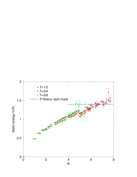
Figure 9: Static Potential for the h2 run, $\kappa=$0.1415

As the spatial extent of the h2 run lattices is considerably smaller (1.7 fm as opposed to 2.4 fm for the 6⁴ lattices) we may expect that the string breaking effects will also be more difficult to see. The static potential measured at various Euclidean times is shown in Fig. 9, and there is as yet no evidence for a flattening of the potential at distances where the errors are still reasonable at larger distances (for lattice times $<\simeq$ 6, or about 1 fm). The expected asymptotic limit (=twice the heavy-light meson mass) is indicated by the dashed line: with the statistics available, this value is only reached when the errors for Wilson lines of temporal extent $T>$4 begin to explode. Much larger statistics will presumably be needed to reach the larger times and distances where stringbreaking will appear on these lattices. We can however use the initial rise of the static potential to extract a rough lattice scale. Extracting a slope from the region $2\leq R\leq 4$, one finds $a$=0.16 fm. A more reliable estimate of the scale can be obtained from the rho mass $M_{\rho}=$0.669(30), obtained by fitting a set of 200 bootstrapped smeared-local rho propagators, as shown in Fig. 10. Using the rho mass to fix the lattice scale gives $a^{-1}$=1.15 Gev, $a$=0.17 fm for the h2 run: as in the case of the 6⁴ runs discussed in Section 3, the scale is not very sensitive to the sea-quark mass in this very light regime, and at $\kappa=$0.1420 we find a rho mass of 0.693(30) in lattice units, giving a lattice scale $a^{-1}$=1.11 GeV.

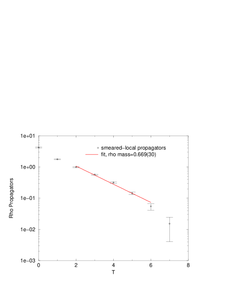
Figure 10: Rho propagator, h2 run, $\kappa=$0.1415

The pion in the h2 ensemble is already very light and autocorrelations are large, typically on the order of 100-150 update steps (with the autocorrelation time growing with Euclidean time) . To analyse the pion propagators, we have therefore binned the smeared-local pion propagators from 99 successive configurations (separated by 50 update steps) into 33 sets of bin size 3 before generating 66 bootstrap propagators for a bootstrap analysis. The corresponding average propagator file and fit is shown in Fig. 11, giving a pion mass of 0.175 in lattice units or 201 MeV. For the h1 run at $\kappa=$0.1420, the pion is even lighter (Fig. 12), but with the limited statistics (80 configurations) available so far the errors at larger Euclidean time are substantial, so an accurate determination of the pion mass in this case is not possible. The h1 propagator is essentially flat for T$>$4, so this case is presumably very close to kappa critical. We should point out that these h1 propagators were obtained by standard conjugate gradient as the stabilized biconjugate gradient routines often fail to converge for very light quarks. Of course, on this smaller lattice finite size effects (which were small on the 2.4 fm lattices for pion masses $>200$ MeV) may well be significant.

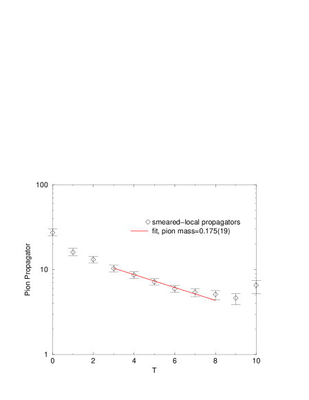
Figure 11: Pion propagator, h2 run, $\kappa=$0.1415

Figure 12: Pion propagator, h1 run, $\kappa=$0.1420

The anomaly in the quenched theory induced in the scalar isovector channel by the incomplete cancellation of the quenched eta-prime double pole [10] is by now well understood. The TDA approximation, while including effects of sea-quark loops up to fairly high off-shellness exactly, does not of course treat valence and sea-quarks identically, so we should expect the appearance of incompletely cancelled double pole contributions in isoscalar channels here also. In the case of the scalar isovector propagator, these contributions are negative metric and result in the propagator going negative at intermediate values of Euclidean time. A similar dip is observed in the scalar isovector propagator obtained form the h2 runs (see Fig. 13), although it is far less pronounced than in the quenched case. In Section 5 we shall see that the same correlator is perfectly well-behaved in the TDA+multiboson exact unquenched algorithm, and indeed allows a statistically accurate extraction of the eta-prime mass without the need for subtraction of disconnected contributions.

Figure 13: Scalar isovector propagator, h2 run, $\kappa=$0.1415

The computational effort required to compute all quark eigenmodes up to a fixed $\Lambda_{TDA}$ on lattices of fixed lattice spacing and growing volume $V$ increases like $V^{\alpha}$ where the exponent $\alpha$ is slightly less than 2. For example, for $\Lambda_{TDA}=$ 450 MeV, we find that for lattices with $a^{-1}=$1.15 GeV, an update step amounts to approximately 1,3.5 and 35 hours on a Pentium-4 2.2GHz processor on 10³x20 (370 eigenvalues), 12³x24 (850 eigenvalues) and 16³x32 (2770 eigenvalues) lattices respectively (cf. Table 2). The scaling properties of the Lanczos code (employing SSE2 acceleration [11]) on a PC cluster with myrinet interface appear very good, so a 16 node cluster with 3GHz processors should be adequate for useful simulations (and comparable in computational effort to the simulations presented here) for even the physically quite large (2.7 fm)³x(5.4 fm) 16³x32 configurations.

Table 2: Volume scaling for TDA calculations

Lattice	$10^{3}\times 20$	$12^{3}\times 24$	$16^{3}\times 32$
time	1 hrs	3.5 hrs	35 hrs
$N_{\rm eig}$	370	850	2770
Lanczos sweeps	28,000	74,000	200,000

In the next section we shall see that the inclusion of the ultraviolet part of the determinant by multiboson techniques increases the computational cost of an update insignificantly, so these estimates hold also for exact algorithms where complete control of the infrared allows probing of the deep chiral limit without critical slowing down of the MonteCarlo dynamics.

5 Exact Unquenched QCD with light quarks: combining TDA and multiboson methods

The evaluation of the ultraviolet contribution to the quark determinant $D_{UV}$ can be accomplished by the Luescher multiboson technique [12], as pointed out previously in [4]. The basic idea of the multiboson technique is to introduce a series of polynomials in a variable $s$ (shortly to be identified with the square of the eigenvalues of $H$, for two degenerate sea-quarks) which converge to $s^{-1}$:

$$\lim_{N\rightarrow\infty}P_{N}(s) = \frac{1}{s},\;0\leq s\leq 1$$ (11)

$$\rm{det}(H^{2}) = \lim_{N\rightarrow\infty}(\rm{det}P_{N}(H^{2}))^{-1}$$ (12)

$$P_{N}(H^{2}) \simeq \prod_{k=1}^{N}((H-\mu_{k})^{2}+\nu_{k}^{2})$$ (13)

$$S_{\rm bosonic} = \sum_{k=1}^{N}\sum_{x}\{|(H-\mu_{k})\phi_{k}(x)|^{2}+\nu_{k}^{2}|\phi_{k}(x)|^{2}\}$$ (14)

Specifically, it is convenient to pick Chebyshev polynomials so that with $u=(s-\epsilon)/(1-\epsilon)$ and $\cos{\theta}=2u-1$, $T^{*}_{r}(u)=\cos{(ru)}$. Then

$$P_{N}(s)\equiv(1+\rho T^{*}_{N+1}(u))/s$$ (15)

with $\rho$ chosen so that $P_{N}(s)$ has a finite limit as $s\rightarrow 0$. With these choices, $sP_{N}(s)$ differs from unity in the interval $\epsilon\leq s\leq 1$ by an amount less than $2(\frac{1-\sqrt{\epsilon}}{1+\sqrt{\epsilon}})^{N+1}$.

The $N$ roots of the polynomial $P_{N}(s)$ typically lie on an ellipse in the complex plane surrounding the spectrum of $H^{2}$ (with $H$ rescaled so that the spectrum of $H^{2}$ lies between 0 and 1). An example, for values of $N$=20,80, is shown in Fig. 8. The essential point is that accurate control of the infrared spectral region requires the number of multiboson fields $N$ to be chosen large (specifically, if we demand a fixed relative error uniformly in the range $\epsilon\leq s\leq 1$, then we must hold $\sqrt{\epsilon}N$ fixed as $\epsilon\rightarrow 0$). This then forces many of the bosonic fields to appear in the action with small “masses” $\nu_{k}$, which in turn leads to critical slowing down in the multiboson sector.

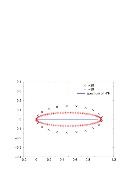
Figure 14: Zeroes of the approximating multiboson polynomial for 20,80 boson fields

Evidently, the exact control over a substantial segment of the infrared quark spectrum provided in the TDA approach suggests that we should be able to reduce substantially the number of multiboson fields, with a corresponding amelioration of the critical slowing down problem. Define a determinantal compensation factor for $N$ multiboson fields as follows

$$D_{CF}(N,N_{\rm eig})\equiv\ln{(\prod_{i=1}^{N_{\rm eig}}\lambda_{i}^{2}P_{N}(\lambda_{i}^{2}))}$$ (16)

where $N_{\rm eig}$ is the number of eigenvalues $\lambda_{i}$ (ordered in absolute value) of $H$ calculated in the TDA approach. We expect that $D_{CF}$ should converge to a well-defined limit once $\lambda_{N_{\rm eig}}^{2}>>\epsilon$. At this point, the compensation factor $D_{CF}$ can be used in an accept/reject step to correct the approximate determinant generated by the multiboson part of the action. To get a quantitative feeling for how rapidly this convergence takes effect, we show two examples in Figs 15,16. In Fig. 15 we consider pairs of adjacent configurations in a simulation in which the 1000 lowest eigenvalues of $H^{2}$ on a $6^{4}$ lattice (with lattice spacing $a\simeq$0.4F) are exactly computed by the Lanczos method, while the multiboson action corresponds to $N=20,\epsilon=0.02$. The plot shows the difference of $D_{CF}$ for two successive configurations (needed for the accept/reject step) as a function of the number of eigenvalues $N_{\rm eig}$ included in the computation of $D_{CF}$. Evidently, the small number of pseudofermion fields used means that the simulated determinant is very inaccurate until several hundred exactly computed eigenvalues are included, at which point the needed determinantal compensation factor converges rapidly. The dependence on $N_{\rm eig}$ is shown for 6 separate pairs of adjacent configurations in the MonteCarlo sequence. In Fig. 16 we show a similar plot for 10³x20 lattices (lattice spacing $a\simeq 0.17$ fm) up to a maximum of $N_{\rm eig}$=600, with $N=50,\epsilon=0.003$.

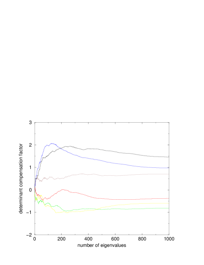
Figure 15: Convergence of determinant correction, 6⁴ lattice ($N=$20,$\epsilon=$0.02)

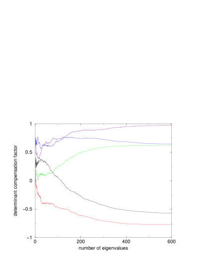
Figure 16: Convergence of determinant correction, 10³x20 lattice ($N=$50,$\epsilon=$0.003)

In order to get a feeling for the basic features of the MonteCarlo dynamics of the combined TDA and multiboson approach described here, we have performed simulations on large, coarse lattices, roughly similar to the ensembles described in Section 3. The gauge action was improved exactly as described there, but with the couplings $\beta_{\rm plaq}$=3.65, $\beta_{\rm trt}$=0.75. The lowest 1000 eigenvalues (corresponding to a TDA scale of about 560 MeV) were computed exactly, and 20 multiboson fields, with $\epsilon=$0.02 were used to compute the UV part of the determinant. The full algorithm breaks into the following steps

1. Multiboson and gauge updates (satisfying detailed balance):
   (a) 1 overrelaxation update of the multiboson fields (with overrelaxation parameter $\omega$=1.9)
   (b) gauge fields update consisting of 10 hit Metropolis, an overrelaxation step and another 10 hit Metropolis update
   (c) 1 overrelaxation update of the multiboson fields

2. Computation of the determinant compensation factor $D_{CF}$, which is then used in an accept/reject step for the new gauge and multiboson fields. The acceptance rate for this step is similar to that in the pure TDA approach, showing little sensitivity to the quark mass in the chiral region (e.g. ranging from 46% at $\kappa=0.1915$, corresponding to a pion mass of 380 MeV to 36% at $\kappa=$0.1930, corresponding to a pion mass of 230 MeV).

At $\kappa$=0.1920, where we have already equilibrated and generated a reasonably large ensemble, we find a lattice scale of $a=0.36$ fm (from string tension measurements) or $a^{-1}\simeq$ 550 MeV. Thus these fully unquenched coarse lattices are roughly similar in size to the ones described in Section 3.

As a simple example of a fully unquenched quantity computed in this approach, where consistent inclusion of all quark eigenmodes is important in avoiding unphysical anomalies, we show in Fig. 17 the pseudoscalar (pion) and scalar isovector propagators obtained from 100 configurations at $\kappa$=0.1920. One obtains a pion mass of 0.60 in lattice units, while the exponential fall of the scalar correlator (corresponding to an intermediate s-wave two-body state of a pion and an $\eta^{\prime}$) corresponds to a mass of 1.94. Subtracting these we find an $\eta^{\prime}$ mass of 1.34 in lattice units, or about 735 MeV, not far from the value of 715 MeV expected in a fictional two-light flavor world [13]. The advantage of this approach to the $\eta^{\prime}$ mass is that the need to subtract disconnected diagrams is completely circumvented! Simulations of this exactly unquenched two-flavor system at lighter quark masses (down to the physical up and down quark masses) are continuing to check the chiral extrapolation of this result, and we are also beginning simulations with 2+1 sea-quark flavors (up, down and strange dynamical quarks) in order to study the $\eta-\eta^{\prime}$ spectrum in a more realistic setting.

Figure 17: Scalar and Pseudoscalar Isovector propagators, fully unquenched

6 Acknowledgements

The authors are grateful for useful conversations with M. diPierro and H. Thacker. The work of A. Duncan was supported in part by NSF grant PHY00-88946. The work of E. Eichten was performed at the Fermi National Accelerator Laboratory, which is operated by University Research Association, Inc., under contract DE-AC02-76CD03000.

References

- [1] S. Duane, A.D. Kennedy, B.J. Pendleton and D. Roweth, Phys.Lett. 195B (1987)216; K. Jansen and C. Liu, Nucl. Phys. B453 (1995) 375.
- [2] Th. Lippert, hep-lat/0203009.
- [3] G.H. Golub and C.F. Loan, Matrix Computations, 2nd edition (Johns Hopkins, 1990); T. Kalkreuter, Comput.Phys.Commun. 95 (1996) 1.
- [4] A. Duncan, E. Eichten and H. Thacker, Phys.Rev. D59 (1999) 014505.
- [5] A. Duncan, E. Eichten, R. Roskies and H. Thacker, Phys. Rev. D60 (1999) 054505.
- [6] A. Duncan, E. Eichten and H. Thacker, Phys. Rev. D63 (2001) 111501.
- [7] M. Alford, W. Dimm, G.P.Lepage, G. Hockney and P.B. Mackenzie, Phys. Lett. B361 (1995) 87.
- [8] A. Duncan, S. Pernice and J. Yoo, Phys. Rev. D65(2002) 094509.
- [9] H.Leutwyler and A. Smilga, Phys. Rev. D46 (1992) 5607.
- [10] W. Bardeen, A. Duncan, E. Eichten, N. Isgur and H. Thacker, Phys.Rev. D65 (2002) 014509.
- [11] M. Luescher, hep-lat/0110007, published in Nucl.Phys.Proc.Suppl. 106(2002) 21.
- [12] M. Luescher, Nucl. Phys. B418 (1994) 637.
- [13] K. Schilling et al, hep-lat/0110077.