Monopole Condensation in full QCD using the Schrödinger Functional

Abstract

We use a lattice thermal partition functional to study Abelian monopole condensation in full QCD with $N_{f}=2$ staggered fermions. We present preliminary results on $16^{3}\times 4$ and $32^{3}\times 4$ lattices.

1 INTRODUCTION

To give a possible explanation of color confinement G. ’t Hooft [1] and S. Mandelstam [2] suggested long time ago that vacuum in gauge theories behaves like a magnetic (dual) superconductor. The dual superconductivity hypothesis relies upon the very general assumption that the dual superconductivity of the ground state is realized if there is condensation of Abelian magnetic monopoles.

1.1 The thermal partition functional

To investigate vacuum structure of lattice gauge theories at finite temperature we introduced [3, 4] a lattice thermal partition functional in presence of a static background field

$$\mathcal{Z}_{T}\left[\vec{A}^{\text{ext}}\right]=\int_{U_{k}(L_{t},\vec{x})=U_{k}(0,\vec{x})=U^{\text{ext}}_{k}(\vec{x})}\mathcal{D}U\,e^{-S_{W}}\,,$$ (1)

$S_{W}$ is the Wilson action, the physical temperature is given by $T=1/aL_{t}$. The functional integration is extended over links on a lattice $L_{s}^{3}\times L_{t}$ with hypertorus geometry and satisfying the constraints ($x_{t}$: temporal coordinate)

$$U_{k}(x)|_{x_{t}=0}=U^{\mathrm{ext}}_{k}(\vec{x})\,,\,\,\,\,\,(k=1,2,3)\,\,,$$ (2)

$U^{\mathrm{ext}}_{k}(x)$ being the lattice version of the external continuum gauge field $\vec{A}^{\mathrm{ext}}(x)=\vec{A}^{\mathrm{ext}}_{a}(x)\lambda_{a}/2$.

$$F[\vec{A}^{\mathrm{ext}}]=-\frac{1}{L_{t}}\ln\frac{\mathcal{Z}_{T}[\vec{A}^{\mathrm{ext}}]}{{\mathcal{Z}}_{T}[0]}\,.$$ (3)

To circumvent the problem of computing a partition function which is the exponential of an extensive quantity, in practical computations we consider $F^{\prime}[\vec{A}^{\mathrm{ext}}]$ the $\beta$-derivative of $F[\vec{A}^{\mathrm{ext}}]$. Indeed this quantity is simply related to the plaquette $U_{\mu\nu}$ ($\Omega=L_{s}^{3}\times L_{t}$):

$$\begin{split}F^{\prime}[\vec{A}^{\mathrm{ext}}]&=\left\langle\frac{1}{\Omega}\sum_{x,\mu<\nu}\frac{1}{3}\,\text{Re}\,{\text{Tr}}\,U_{\mu\nu}(x)\right\rangle_{0}\\ &-\left\langle\frac{1}{\Omega}\sum_{x,\mu<\nu}\frac{1}{3}\,\text{Re}\,{\text{Tr}}\,U_{\mu\nu}(x)\right\rangle_{\vec{A}^{\mathrm{ext}}}\,,\end{split}$$ (4)

where the subscripts on the averages indicate the value of the external field.

1.2 Including fermions

We are interested in gauge systems at thermal equilibrium in presence of a static (time-independent) external background field. So that in presence of dynamical fermions Eq. (1) becomes:

$$\begin{split}&\mathcal{Z}_{T}\left[\vec{A}^{\text{ext}}\right]=\\ &\int_{U_{k}(L_{t},\vec{x})=U_{k}(0,\vec{x})=U^{\text{ext}}_{k}(\vec{x})}\mathcal{D}U\,{\mathcal{D}}\psi\,{\mathcal{D}}\bar{\psi}e^{-(S_{W}+S_{F})}\,,\end{split}$$ (5)

where we integrate on fermionic fields without any constraint. As usual we impose on fermionic fields periodic boundary conditions in the spatial directions and antiperiodic boundary conditions in the temporal direction.

1.3 Detecting monopole condensation

Abelian monopole condensation can be detected using order/disorder parameters [5, 6, 7]. The disorder parameter is related to the monopole free energy and is defined by means of the thermal partition function in presence of the Abelian monopole background field:

$$\mu=e^{-F_{\text{mon}}/T_{\text{phys}}}=\frac{\mathcal{Z}_{T}\left[\mathbf{A}^{\text{mon}}\right]}{\mathcal{Z}_{T}[0]}\,,$$ (6)

$F_{\text{mon}}$ is the free energy to create a monopole. If there is condensation $F_{\text{mon}}$ is finite and $\mu\neq 0$. Note that since our disorder parameter $\mu$ has been defined in terms of the thermal partition functional $\mathcal{Z}_{T}$ that is gauge-invariant for time-independent gauge transformations of the external background fields gauge fixing is not needed to perform the Abelian projection in the case of Abelian background fields.

2 ABELIAN MONOPOLES IN FULL QCD

2.1 Definition

In the continuum the magnetic monopole field with the Dirac string in the direction $\vec{n}$ is

$$e\vec{b}({\vec{x}})=\frac{n_{\mathrm{mon}}}{2}\frac{\vec{x}\times\vec{n}}{|\vec{x}|(|\vec{x}|-\vec{x}\cdot\vec{n})}\,,$$ (7)

where, according to the Dirac quantization condition, $n_{\mathrm{mon}}$ is an integer and $e$ is the electric charge magnetic charge = $n_{\mathrm{mon}}/2e$.

For SU(3) gauge theory the maximal Abelian group is U(1)$\times$U(1), therefore we may introduce two independent types of Abelian monopoles associated respectively to the $\lambda_{3}$ and $\lambda_{8}$ diagonal generators of SU(3). We shall consider here the $\lambda_{3}$ Abelian monopole field. On the lattice it is given by ($(X_{1},X_{2},X_{3})$ monopole coordinates)

$$U_{1,2}^{\text{ext}}(\vec{x}) =\begin{bmatrix}e^{i\theta^{\text{mon}}_{1,2}(\vec{x})}&0&0\\ 0&e^{-i\theta^{\text{mon}}_{1,2}(\vec{x})}&0\\ 0&0&1\end{bmatrix}\,,$$

$$U^{\text{ext}}_{3}(\vec{x}) ={\mathbf{1}}\,,$$ (8)

$$\theta^{\text{mon}}_{1,2}(\vec{x}) =\mp\frac{n_{\text{mon}}}{4}\frac{(x_{2,1}-X_{2,1})}{|\vec{x}_{\text{mon}}|}\frac{1}{|\vec{x}_{\text{mon}}|-(x_{3}-X_{3})}\,.$$

2.2 Numerical simulations

We used the standard HMC R-algorithm for two degenerate flavors of staggered fermions with a quark mass $am=0.075$ (at this value of the mass and $N_{T}=4$ $\rightarrow$ $\beta_{c}\sim 5.35$ [8]). We have collected about 2000 thermalized trajectories for each value of $\beta$ at $L_{s}=16$ and about 500 thermalized trajectories for each value of $\beta$ at $L_{s}=32$. Each trajectory consists of $125$ molecular dynamics steps and has total length $1$. The computer simulations have been performed on the APEmille crate at INFN/Bari.

2.3 Numerical results

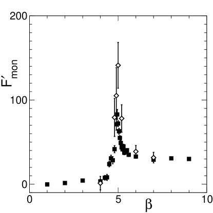
Figure 1: The $\beta$-derivative of the monopole free energy $F^{\prime}_{\text{mon}}$ on a $L_{s}^{3}\times 4$ lattice for 2 flavors QCD (full squares and open diamonds refer respectively to $L_{s}=16$ and $L_{s}=32$).

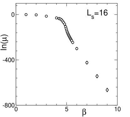
Figure 2: The logarithm of the disorder parameter Eq. (6) for 2 flavors QCD and $L_{s}=16$.

In Fig. 1 we compare $F^{\prime}_{\text{mon}}$ in the 2 flavors full QCD case for two different spatial volumes. Data in the weak and strong coupling regions agree within statistical errors. On the other hand the signal at the peak value gets increased going to a larger spatial volume.

Observing that $F_{\text{mon}}=0$ at $\beta=0$, we may obtain $F_{\text{mon}}$ from $F^{\prime}_{\text{mon}}$ by a numerical integration in $\beta$ and from Eq. (6) we are able to estimate the disorder parameter $\mu$. Fig. 3 shows that $\ln\mu=0$ in the confined phase, i.e. the free energy required to create an Abelian monopole in the QCD vacuum is zero and therefore Abelian monopoles condense in the confined phase.

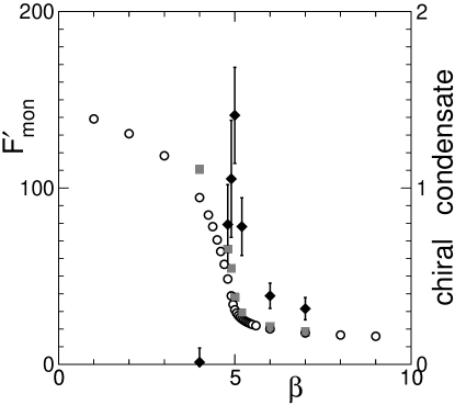
Figure 3: $F^{\prime}_{\text{mon}}$ in 2 flavors QCD and $L_{s}=32$ (full diamonds) compared with chiral condensate at $L_{s}=16$ (open circles) and $L_{s}=32$ (full grey squares).

Fig. 4 displays $F^{\prime}_{\text{mon}}$ in the 2 flavors full QCD case and $L_{s}=32$ compared with the chiral condensate. The peak in $F^{\prime}_{\text{mon}}$ corresponds to the drop of the chiral condensate.

3 CONCLUSIONS

Using a thermal partition functional in presence of an external Abelian monopole background field we simulate 2 staggered flavors full QCD on a $L_{s}^{3}\times 4$ lattice. We find that Abelian monopoles condense in the spontaneously broken chiral symmetry phase of 2 flavors full QCD. This is consistent with similar results found in Ref. [9] For a better understanding of Abelian monopole condensation in full QCD we expect to perform new simulations at different values of the masses and of the flavor numbers as well a finite size scaling analysis.

References

- [1] G. ’t Hooft, High Energy Physics, EPS International Conference, Palermo, 1975.
- [2] S. Mandelstam, Phys. Rept. 23 (1976) 245.
- [3] P. Cea and L. Cosmai, JHEP 11 (2001) 064.
- [4] P. Cea and L. Cosmai, Phys. Rev. D62 (2000) 094510, hep-lat/0006007.
- [5] L.P. Kadanoff and H. Ceva, Phys. Rev. B3 (1971) 3918.
- [6] E.H. Fradkin and L. Susskind, Phys. Rev. D17 (1978) 2637.
- [7] A. Di Giacomo and G. Paffuti, Phys. Rev. D56 (1997) 6816, hep-lat/9707003.
- [8] JLQCD, S. Aoki et al., Phys. Rev. D57 (1998) 3910, hep-lat/9710048.
- [9] J.M. Carmona, M. D’Elia, L. Del Debbio, A. Di Giacomo, B. Lucini, and G. Paffuti, Phys. Rev. D66 (2002) 011503, hep-lat/0205025.