Panel discussion on chiral extrapolation of physical observables

Abstract

This is an approximate reconstruction of the panel discussion on chiral extrapolation of physical observables. The session consisted of brief presentations from panelists, followed by responses from the panel, and concluded with questions and comments from the floor with answers from panelists. In the following, the panelists have summarized their statements, and the ensuing discussion has been approximately reconstructed from notes.

1 Introduction

Sharpe: It has become apparent from many talks at this conference that chiral extrapolation is an issue of great practical importance. Different approaches are being tried, and it is certainly timely to have a general discussion of the issue. In order to focus the discussion, I sent the panelists a draft list of key questions to focus their thoughts as they were preparing their remarks. These questions have evolved as a result of feedback, and my present version (in no particular order) is as follows.

1. How small does the quark mass need to be to use chiral perturbation theory ($\chi$PT)?

2. Do we need to use fermions with exact chiral symmetry to reach the region where $\chi$PT applies?

3. What fit forms should we use outside the chiral region?

4. Is the strange quark light enough to be in the chiral regime?

5. Is it necessary to include $O(a,a^{2})$ effects in the chiral Lagrangian?

6. Can we use (present or future) partially quenched simulations to obtain quantitative results for physical parameters?

7. Can we use quenched simulations to give quantitative results for physical parameters?

8. Is it possible and/or desirable to work at $m_{q}=0$?

2 Presentations

Bernard: At this conference, and in the recent literature, several groups have emphasized a key point about chiral extrapolations: Over the typical current range of lattice values for the light quark masses, the data for many physical quantities is quite linear. Yet linear extrapolations will miss the chiral logarithms that we know are present and therefore may introduce large systematic errors into the results. JLQCD [1], Kronfeld and Ryan [2], and Yamada’s review talk here [3] have stressed the relevance of this point for heavy-light decay constants; while the Adelaide group [4, 5, 6, 7, 8] has brought out the same point in the context of baryon physics. All these groups deserve a lot of credit for bringing this important issue to the fore.

Now the question is: “What are we going to do about it?” Attempts to extract the logarithms directly in the current typical mass range are in my opinion doomed to failure: The extreme linearity of the data indicates, at best, that higher order terms must be contributing in addition to the logarithms, or, at worst, that we are out of the chiral regime altogether. The only real solution is to go to lower quark masses. We need to be well into the chiral regime, to see the logs and make controlled fits including this known chiral physics. My rough guess in the heavy-light decay constant case is that we need $m_{\pi}/m_{\rho}\approx 0.3$, or at best $m_{\pi}/m_{\rho}{\mathrel{\raise 2.0pt\hbox to8.0pt{\raise-5.0pt\hbox{$\sim$}\hss{$<$}}}}0.4$. The latter range may be reachable, with significant work, with Wilson-type fermions; while the former may require, at least in the near term, staggered fermions. The use of staggered light valence quarks in heavy-light simulations, as was suggested by Wingate at Lattice 2001 [9], should make the chiral regime for that problem accessible very soon.

A different approach has been advocated by the Adelaide group. They say we can take into account the chiral logarithms in the current range of masses by modeling the turn-off of chiral logarithms with a quantity-dependent cutoff that represents the “core” of the object under study. I have nothing against modeling per se; I think it can be an excellent tool to gain qualitative insight into the physics. What I think is wrong, or at least wrong-headed, about the Adelaide approach is the suggestion that one can use it to extract reliable quantitative answers with controlled errors. Extraction of such answers is after all why we are doing lattice physics in the first place.

The Adelaide model introduces a single parameter, the core size, to describe the very complicated real physics involving couplings to all kinds of particles — $\rho$’s, $\sigma$’s, etc. — as one moves out of the chiral regime. The change in their results when they change the parameter by some amount or vary the functional form at the cutoff is simply not a reliable, systematically improvable error. In other words, their model is an uncontrolled approximation.

Suppose, however, one phrases the question in the following way: “Given some lattice data in the linear regime, are you likely to get closer to the right answer with a linear fit, or with an Adelaide form that interpolates between linear behavior and the known chiral behavior at low mass?” Phrased that way, my answer would be, “the Adelaide form.” But the problem is that, while you are most likely closer to the right answer, you do not know the size of the errors — unless you know the right answer to begin with! In my opinion, the linear fit is a “straw man” alternative. The real alternative is to go to lighter masses and fit to the known chiral form. This approach, and this approach only, will produce controlled, systematically improvable errors: To improve, just go to higher order in the chiral expansion or to still lighter masses.

Now if we want to go to lighter masses, I would argue that the easiest way to do so is by using staggered fermions. Dynamical staggered fermions are very fast, and they have an exact lattice chiral symmetry. However, as you know, many of the other staggered symmetries are broken at finite lattice spacing.

First of all, let me talk about nomenclature. I would like to advocate here the use of the word “taste” to describe the 4 internal fermion types inherent in a single staggered field. Taste symmetry is violated on the lattice at ${\cal O}(a^{2})$ but becomes exact in the continuum limit. I reserve the word “flavor” for different staggered fields, which have an exact lattice symmetry (in the equal mass case) that mixes them. For example, MILC is doing simulations with 3 flavors ($u$, $d$, and $s$) with $m_{u}=m_{d}\not=m_{s}$. Normally each flavor would have 4 tastes, but we do the usual trick of taking the fourth root of the determinant to get a single taste per flavor. Of course this is ugly and non-local, and one must test that there are no problems introduced in the continuum limit.

I find it useful to think about the effects of taste symmetry breaking as just a more complicated version of “partial quenching” [10]. Sharpe and Shoresh [11] have taught us that, as long as a theory has the right number of sea quarks (3), the chiral parameters are physical even if the masses of the quarks are not physical, and even if the valence and sea quark masses are different (i.e., even if the theory is partially quenched). With three staggered flavors and $\root 4 \of{\rm Det}$’s, the theory is, I believe, still in the right sector and has physical chiral parameters. But it is like a theory with 12 sea quarks, each with $1/4$ weight, rather than 3 normal flavors.

In order to extract the physical chiral parameters from an ordinary 3-flavor partially quenched theory, we need the correct functional forms calculated in partially quenched chiral perturbation theory. Similarly, in order to extract the physical chiral parameters from a theory of 3 staggered flavors with $\root 4 \of{\rm Det}$’s, we need the functional forms calculated in a staggered chiral perturbation theory (S$\chi$PT). This includes the effect of the ${\cal O}(a^{2})$ taste violations.

The starting point of S$\chi$PT is the chiral Lagrangian of Lee and Sharpe [12], which is the low energy effective theory for a single staggered field, correct to ${\cal O}(a^{2})$. To apply it to the case of interest, one must generalize to 3 flavors (which turns out to be non-trivial), calculate relevant quantities at 1-loop, and the adjust for the effect of taking $\root 4 \of{\rm Det}$’s. Student Chris Aubin and I have done this for $m_{\pi}^{2}/(2\hat{m})$ and $m_{K}^{2}/(\hat{m}+m_{s})$ [13]. ($\hat{m}$ is the average $u,d$ quark mass.) One can fit the MILC data very well with our results. We are in the process of extending this work to $f_{\pi}$, $f_{K}$ and heavy-light decay constants, as well as allowing for different valence and sea quark masses.

Hashimoto: Since the computational cost required to simulate dynamical quarks grows very rapidly as the sea quark mass is decreased, controlled chiral extrapolation is crucial to obtain reliable predictions for physical quantities. Through this short presentation I would like to share our experience with chiral extrapolations obtained from the unquenched simulation being performed by the JLQCD collaboration using nonperturbatively $O(a)$-improved Wilson fermions on a relatively fine lattice, $a\sim$ 0.1 fm. Further details are presented in a parallel talk [14].

The strategy we have in mind when we do the chiral extrapolation is to use chiral perturbation theory ($\chi$PT) as a theoretical guide to control the quark mass dependence of physical quantities. For this strategy to work one has to push the sea quark mass as light as possible and test whether the lattice data are described by the one-loop $\chi$PT formula. (The lowest order $\chi$PT prediction usually does not have quark mass dependence.) If so, chiral extrapolation down to the physical pion mass is justified.

In full QCD $\chi$PT predicts the chiral logarithm with a definite coefficient depending only on the number of active flavors, which gives a non-trivial test of the unquenched lattice simulations. For example the PCAC relation $M_{\mathrm{SS}}^{2}\simeq 2B_{0}m_{S}$ is given as

$$\frac{M_{\mathrm{SS}}^{2}}{2B_{0}m_{S}}=1+\frac{1}{N_{f}}y_{\mathrm{SS}}\ln y_{\mathrm{SS}}$$ (1)

$$+y_{\mathrm{SS}}[(2\alpha_{8}-\alpha_{5})+N_{f}(2\alpha_{6}-\alpha_{4})]$$

for $N_{f}$ flavors of degenerate quarks with a mass $m_{S}$ and $y_{\mathrm{SS}}=2B_{0}m_{S}/(4\pi f)^{2}$. Similar expression for the pseudoscalar meson decay constant is

$$\frac{f_{SS}}{f}=1-\frac{N_{f}}{2}y_{\mathrm{SS}}\ln y_{\mathrm{SS}}+\frac{y_{\mathrm{SS}}}{2}[\alpha_{5}+N_{f}\alpha_{4}].$$ (2)

The coefficient of the chiral log term is fixed, while the low energy constants $\alpha_{i}$ are unknown. Figure 1 shows the comparison of lattice data with (1), and it is unfortunately clear that the lattice result does not reproduce the characteristic curvature of the chiral logarithm. The same is true for the pseudoscalar meson decay constant, and the ratio test using partially quenched $\chi$PT leads to the same conclusion [14].

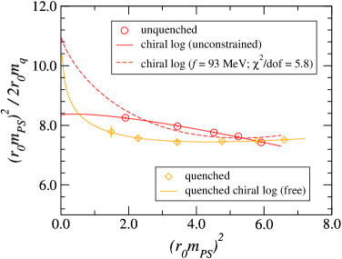
Figure 1: Test of the one-loop $\chi$PT formula from the JLQCD collaboration.

The most likely reason is that the dynamical quarks in our simulations are still too heavy. In fact, the corresponding pseudoscalar meson mass ranges from 550 to 1,000 MeV, for which we do not naively expect that $\chi$PT works, especially at the high end. Our analysis of the partially quenched data suggests that a meson mass as low as 300 MeV is necessary to be consistent with one-loop $\chi$PT.

Let us now discuss the systematic uncertainty in the chiral extrapolation. Since we know that the $\chi$PT is valid for small enough quark masses, the chiral extrapolation has to be consistent with the one-loop $\chi$PT formula at least in the chiral limit. If we assume that the chiral logarithm dominates only below a scale $\mu$, a possible model is to take the one-loop $\chi$PT formula below $\mu$ while using a conventional polynomial fitting elsewhere. Both functions may be connected so that their value and first derivative match at the scale $\mu$. The scale $\mu$ is unknown, though we naively expect that $\mu$ is around 300–500 MeV. Therefore, we should consider the dependence on $\mu$ in a wider range, say 0–1,000 MeV, as an indication of the systematic error in the chiral extrapolation. A plot showing these fitting curves is presented in [14].

Another possible functional form is that suggested by the Adelaide-MIT group [15]. They propose using the one-loop $\chi$PT formula calculated with a hard momentum cutoff $\mu$, which amounts to replacing the chiral log term $m_{\pi}^{2}\ln(m_{\pi}^{2}/\mu^{2})$ by $m_{\pi}^{2}\ln(m_{\pi}^{2}/(m_{\pi}^{2}+\mu^{2}))$. It is a model in the sense that we use it above the cutoff scale $\mu$. Fits to the pion decay constant are shown in Figure 2. The fit curves represent the model with $\mu$ = 0, 300, 500, and $\infty$ MeV. Since we do not have a solid theory to choose the cutoff scale $\mu$, the variation of the chiral limit should be taken as the systematic uncertainty, whose size is of order of $\pm$10%.

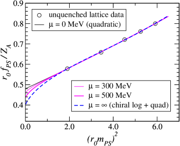
Figure 2: Uncertainty in the chiral extrapolation of pion decay constant.

The large uncertainty associated with the chiral extrapolation as discussed above has not attracted much attention, partly because most simulations have been done in the quenched approximation, for which the chiral behavior of physical quantities is quite different. In contrast, in unquenched QCD, confirming the predictions of $\chi$PT gives a non-trivial test of the low energy behavior obtained from lattice calculations. For pion or kaon physics it is essential to perform the lattice simulation in a region where $\chi$PT is applicable, since the physics analysis often relies on $\chi$PT.

State-of-the-art unquenched lattice simulations using Wilson-type fermions are still restricted to the large sea quark mass region $\geq m_{s}/2$, for which we do not find an indication of the one-loop chiral logarithm. This means that there could be a sizable systematic uncertainty in the chiral extrapolation. I have discussed the example of the pion decay constant; a similar analysis is underway for the heavy-light decay constants and light quark masses.

Pallante: Chiral extrapolation of weak matrix elements and in particular kaon matrix elements (i.e. $B_{K}$, $K\to 2\pi$ decays, semileptonic kaon decays) is a very delicate issue. One of the most difficult tasks still remains the calculation of $\langle\pi\pi|O_{W}|K\rangle$ matrix elements, where $O_{W}$ is a weak four-quark effective operator at scales $\mu<M_{W}$, typically $\mu\sim m_{c}$.

Since elastic (soft) final state interactions (FSI) of the two pions are large especially in the total isospin zero channel (see [16] and refs. therein), it is mandatory to overcome the Maiani-Testa no-go theorem [17] and to include the bulk of FSI effects directly in the lattice measurement of kaon matrix elements, while keeping under control residual corrections through the use of Chiral Perturbation Theory ($\chi$PT).

A considerable step forward in this respect has been made in refs. [18, 19], where it has been shown that the physical matrix element can be extracted from the measurement of an Euclidean correlation function at finite volume. The finite volume matrix element is converted to the infinite volume one via a multiplicative universal factor [18] (denoted as LL factor in the following), i.e. only depending on the quantum numbers of the $\pi\pi$ final state.

There are three main reasons why $\chi$PT is needed, at least up to next-to-leading order (NLO), in extracting the physical $\langle\pi\pi|O_{W}|K\rangle$ matrix element from a lattice Euclidean correlation function: 1) Lattice simulations are presently performed at unphysical values of light quark masses, so that $\chi$PT is needed to parameterize mass dependences and perform the extrapolation to their physical value, provided it is applicable at the values of quark masses used on the lattice. 2) Lattice simulations may be done with unphysical choices of the kinematics, simpler than the physical one, and again $\chi$PT is needed for the extrapolation. 3) $\chi$PT is an appropriate tool to monitor in a perturbative manner the size of systematic errors due to a) (partial) quenching, b) finite volume and c) non-zero lattice spacing [20].

It is also important to note that the possibility of computing lattice matrix elements with choices of momenta and masses different from the physical ones is a very powerful method, once we want to determine the low-energy constants (LEC) which appear in the chiral expansion of observables at NLO. By varying momenta, and masses, we can increase the number of linear combinations of LEC that can be extracted from a lattice computation.

A possible strategy for the direct measurement of $\langle\pi\pi\left|O_{W}\right|K\rangle$ matrix elements has been formulated in ref. [21], specifically for the $\Delta I=3/2$ case (see also ref. [22] at this conference). This strategy is general, and can be applied also to the $\Delta I=1/2$ case. It is as follows: 1) evaluate the Euclidean correlation function $C_{\vec{q}_{1}\vec{q}_{2}}=\langle 0\left|\pi_{\vec{q}_{1}}(t_{1})\pi_{\vec{q}_{2}}(t_{2})O_{W}(0)K_{\vec{0}}(t_{K})\right|0\rangle$ at fixed physics, i.e. at fixed two-pion total energy at finite volume; 2) divide by the appropriate source (sink) correlation functions at finite volume. This step produces the finite volume matrix element $\left|{}_{V}\langle\pi\pi\left|O_{W}(0)\right|K\rangle{}_{V}\right|$, and 3) multiply it by the universal LL factor to get the infinite volume amplitude: $\left|\langle\pi\pi\left|O_{W}(0)\right|K\rangle\right|^{2}=LL\times\left|{}_{V}\langle\pi\pi\left|O_{W}(0)\right|K\rangle{}_{V}\right|^{2}$. 4) If not able to apply the procedure 1) to 3) directly for the physical kinematics, then apply the procedure for an alternative choice of the kinematics that is sufficient to fully determine the physical amplitude at NLO in $\chi$PT. Two such choices for the $\Delta I=3/2$ case are the SPQR kinematics [23], where one of the two pions carries a non-zero three-momentum, and the strategy proposed in ref. [24], using the combined measurements of $K\to\pi\pi$ at $m_{K}=2m_{\pi}$ and $m_{K}=m_{\pi}$, $K\to\pi$ at non-zero momentum, $K\to 0$ and $K^{0}-\bar{K}^{0}$ transition amplitudes. The second strategy is also sufficient for the $\Delta I=1/2$ case, while the SPQR kinematics for $\Delta I=1/2$ is under investigation. Also, the LL factor derived in [18] is only applicable to the center-of-mass frame, while its generalization to a moving frame has not yet been derived (see ref. [21] for a discussion).

Unfortunately, most realistic lattice simulations are still performed in the quenched approximation or, at best, in the partially quenched approximation with two or three dynamical (sea) flavors. The loss of unitarity due to (partial) quenching of $SU(3)_{L}\times SU(3)_{R}$ chiral group has dramatic consequences in the $I=0$ channel of $K\to\pi\pi$ amplitudes [25, 26]. Loss of unitarity implies the failure of Watson’s theorem and Lüscher’s quantization condition. As a consequence, the FSI phase extracted from the quenched weak amplitude is no longer universal (i.e. it may also depend on the weak operator $O_{W}$) and finite volume corrections of quenched weak matrix elements among physical states are not universal (i.e. the universality of the LL factor does not work as in the full theory) [26].

The reason why the $I=0$ case is a peculiar one is that the rescattering diagram of the two final state pions (the one producing the phase of the amplitude) is modified by (partial) quenching already at one loop in $\chi$PT. This is not the case for $I=2$ however, where the rescattering diagram is unaffected by quenching at least to one loop in $\chi$PT. This guarantees the applicability of the direct strategy to the $I=2$ channel also in the quenched approximation, at least up to one loop in the chiral expansion.

Another consequence of (partial) quenching is the contamination of QCD-LR penguin operators, like $Q_{6}$, by new non-singlet operators [27] which appear at leading order in the chiral expansion (i.e. order $p^{0}$, even enhanced respect to the order $p^{2}$ singlet operator). This contamination does not affect $\Delta I=3/2$ transitions, being pure $\Delta I=1/2$.

Given the above picture, a few conclusions can be drawn. At present, $\chi$PT plays a crucial role in the extrapolation of lattice weak matrix elements to their physical value, or to the chiral limit. However, the applicability of $\chi$PT at the lowest orders (typically up to NLO) in the extrapolation procedure is guaranteed only for sufficiently light values of lattice meson masses. This means that one should work in a region of quark masses sufficiently far below the first relevant resonance. The situation can be further complicated by the presence of FSI effects, especially in the $I=0$ channel. These effects can be either analytically resummed [16] or the bulk of them be directly included into the finite volume lattice matrix element. Most critical appears the situation in the presence of quenching, due to the lack of unitarity. For $\Delta I=3/2$ matrix elements, strategies proposed for a direct measurement with unquenched simulations can still be used in a quenched simulation at least up to NLO in the chiral expansion. This is no longer true for $\Delta I=1/2$ matrix elements. In this case, quenching and partial quenching affect universal properties of the weak amplitude already at one loop in $\chi$PT, and in addition produce a severe contamination of QCD-LR penguin operators with new non-singlet operators. However, those problems disappear in the partially quenched case with $N_{sea}=N_{valence}$ and $m_{sea}=m_{valence}$, where partially quenched correlation functions reproduce those of full QCD[10, 11].

Leinweber: Until recently, it was difficult to establish the range of quark masses that can be studied using chiral perturbation theory ($\chi$PT) [28]. Now, with the advent of lattice QCD simulation results approaching the light quark mass regime, considerable light has been shed on this important question [29, 7, 15, 30, 31, 32, 4]. It is now apparent that current leading-edge dynamical-fermion lattice-QCD simulation results lie well outside the applicable range of traditional dimensionally-regulated (dim-reg) $\chi$PT in the baryon sector.

The approach of the Adelaide group is to incorporate the known or observed heavy quark behavior of the observable in question and the known nonanalytic behavior provided by $\chi$PT within a single functional form which interpolates between these two regimes. The introduction of a finite-range regulator designed to describe the finite size of the source of the meson cloud of hadrons achieves this result. The properties of the meson-cloud source are parameterized and the values of the parameters are constrained by lattice QCD simulation results. Without such techniques, one cannot connect experiment and current dynamical-fermion lattice-QCD simulation results for baryonic observables.

The use of a finite-range regulator might be confused with modeling. However, it is already established that $\chi$PT can be formulated model independently using finite-range regulators such as a dipole [33]. The coefficients of leading-nonanalytic (LNA) terms are model independent and unaffected by the choice of regulation scheme. The explicit dependence on the finite-range regulation parameter is absorbed into renormalized coefficients of the chiral Lagrangian.

The shape of the regulator is irrelevant to the formulation of $\chi$PT. However, current lattice simulation results encourage us to look for an efficient formulation which maximizes the applicable pion-mass range accessed via one- or two-loop order. An optimal regulator (perhaps motivated by phenomenology) will effectively re-sum the chiral expansion encapsulating the physics in the first few terms of the expansion. The approach is systematically improved by simply going to higher order in the chiral expansion. Our experience with dipole and monopole vertex regulators indicates that the shape of the regulator has little effect on the extrapolated results, provided lattice QCD simulation results are used to constrain the optimal regulator parameter on an observable-by-observable basis [8].

In order to correctly describe QCD, the coefficients of nonanalytic terms must be fixed to their known model-independent values. This practice differs from current common practice within our field where these coefficients are demoted to fit parameters and optimized using lattice simulation results which lie well beyond the applicable range of traditional dim-reg $\chi$PT. The failure of the approach is reflected in fit parameters which differ from the established values of $\chi$PT by an order of magnitude [7] spoiling associated predictions [8, 34].

I will focus on the extrapolation of the nucleon mass as it encompasses the important features which led to subsequent developments [29, 15, 30, 31, 32] required to extrapolate today’s lattice QCD results. Figure 3 displays the results of a finite-range chiral expansion [35] of the nucleon mass (solid curve) constrained by dynamical-fermion simulation results from UKQCD [36] (open symbols) and CP-PACS [37] (closed symbols). The expression for the nucleon mass

$$M_{N} = c_{0}+c_{2}\,m_{\pi}^{2}-{{3\,g_{A}^{2}\over 32\,\pi\,f_{\pi}^{2}}}\times$$

$${2\over\pi}\,\left[m_{\pi}^{3}\;{\rm arctan}\,\left({{\Lambda\over m_{\pi}}}\right)+{\Lambda^{3}\over 3}-\Lambda\,m_{\pi}^{2}\right]\,,$$

arises from the one-loop pion-nucleon self-energy of the nucleon, with the momentum integral regulated by a sharp cutoff. The lattice simulation results constrain the optimal regulator parameter, $\Lambda$, to 620 MeV. Of course it is desirable to use more realistic regulators such as a dipole form when keeping only one-loop terms of the chiral expansion.

Figure 3: The finite-range regulated expansion of the nucleon mass (solid curve) and its perturbative chiral (curves (i) through (iv) and heavy-quark (curves (v) through (vii)) expansions [35]. Details of each curve may be found in the text.

For small $m_{\pi}$ the standard LNA behavior of $\chi$PT is obtained with the correct coefficient. For large $m_{\pi}$, the arctangent tends to zero and suppresses the nonanalytic behavior in accord with the large quark masses involved. The scale of the regulator $\Lambda$ has a natural explanation as the scale at which the pion Compton wave length emerges from the hadronic interior. It is the scale below which the neglected extended structure of the effective fields becomes benign.

The valid regime of the truncated expansion of $\chi$PT is the regime in which the choice of regulator has no significant impact. To gain further insight into the validity of the truncated expansion of traditional dim-reg $\chi$PT, one can perform a power series expansion of the arctangent in terms of $m_{\pi}/\Lambda$ and keep terms only to a given power [35]. The dim-reg expansion of (2) for small $m_{\pi}/\Lambda$ is provided by curves (i) through (iv) in Fig. 3. Curve (i) contains terms to order $m_{\pi}^{2}$, and (ii) to order $m_{\pi}^{3}$. This is the correct implementation of the LNA behavior of $\chi$PT. The behavior dramatically contrasts the common but erroneous approach discussed above. The applicable range of traditional dim-reg $\chi$PT to LNA order for the nucleon mass is merely $m_{\pi}<200$ MeV. Incorporation of the next analytic $m_{\pi}^{4}$ term extends this range to 400 MeV. Curve (iv) illustrates the effect of including the $m_{\pi}^{6}$ term of the expansion.

Within the range $m_{\pi}^{2}<0.15\ {\rm GeV}^{2}$, dim-reg $\chi$PT requires three analytic-term coefficients, $c_{0}$, $c_{2}$ and $c_{4}$ (the coefficient of $m_{\pi}^{4}$), to be constrained by lattice QCD simulation results. The Adelaide approach optimizes $c_{0}$, $c_{2}$ and $\Lambda$ in place of $c_{4}$. Tuning the regulator parameter is not modeling. Instead, optimization of the regulator provides the promise of suppressing $c_{4}$ and higher-order terms. One can understand how this approach works through the consideration of how the regulator models the physics behind the effective field-theory, but such descriptions do not undermine the rigorous nature of the effective field theory.

While the Adelaide approach of (2) is $\chi$PT, it is the current state of lattice QCD simulation results that demand the parameters of the chiral expansion be determined in other ways. The extension to generalized Padé approximates [29, 30, 31, 32], modifications of log arguments [15] and meson-source parameterizations [7, 8, 34, 5] are methods to constrain the chiral parameters with today’s existing lattice QCD simulation results.

Traditional dim-reg $\chi$PT to one loop knows nothing about the extended nature of the meson cloud source. As there is no other mechanism to incorporate this physics, the expansion fails catastrophically if it is used beyond the applicable range. Moreover, convergence of the dim-reg expansion is slow as large errors associated with short-distance physics in loop integrals (not suppressed in dim-reg $\chi$PT) must be removed by equally large analytic terms. These points are made obvious by examining the predictions of the power series expansions (curves (i) through (iv)) of Fig. 3 at $m_{\pi}^{2}=0.3\ {\rm GeV}^{2}$. Curve (ii) incorporating terms to $m_{\pi}^{3}$ is particularly amusing.

In contrast, the optimal finite-range regulation of the Adelaide Group provides an additional mechanism for incorporating finite-size meson-cloud effects beyond that contained explicitly in the leading order terms of the dim-reg expansion. The finite-size regulator effectively re-sums the chiral expansion, suppressing higher-order terms and providing improved convergence. The net effect is that a catastrophic failure of the chiral expansion is circumvented and a smooth transition to the established heavy quark behavior is made.

It is time for those advocating standard chiral expansions to use them with the established model-independent coefficients and in a regime void of catastrophic failures; a regime that can be extended using finite-size regulators. The approach of the Adelaide Group provides a mechanism for confidently achieving these goals with the cautious conservatism vital for the future credibility of our field.

Lepage: This is a remarkable time in the history of lattice QCD. For the first time we appear to have an affordable procedure for almost realistic unquenching. Improved staggered quarks are so efficient that the MILC collaboration has already produced thousands of configurations with small lattice spacings and three flavors of light quark: one at the strange quark mass, and the other two at masses of order $1/5$ or $1/7$ or less of the strange quark mass. For the first time we can envisage a broad range of phenomenologically relevant lattice calculations, in such areas as $B$ physics and hadronic structure, that are precise to within a few percent and that must agree with experiment.

Chiral extrapolations are likely to be one of the largest sources of systematic error in such high-precision work. The MILC collaboration is already working at much smaller light-quark masses than have been typical in the field; there is little doubt that these masses are small enough for a viable chiral perturbation theory. And partial quenching provides a powerful tool for determining the needed chiral parameters. Such a systematic approach is essential for high precision.

As discussed by Claude Bernard, the most significant complication in the chiral properties of improved staggered quarks comes from their “taste-changing” interactions. Crudely speaking these generate a non-zero effective quark mass, proportional to $a^{2}$, even for zero bare quark mass. This effect is perturbative in QCD, and can be removed by modifying the quark action. It can also be measured directly in simulations; we should know shortly how significant it is for typical lattice spacings.

An important aspect of high-precision lattice QCD is choosing appropriate targets. High-precision work in the near future will focus on stable or nearly stable hadrons. It will be much harder to achieve errors smaller than 10–20% for processes that involve unstable hadrons such as the $\rho$ or $K^{*}$. One might try to extrapolate through the decay threshold, but thresholds are intrinsically nonanalytic and so extrapolation is very unreliable. Hadrons very near to thresholds, such as the $\phi$ or the $\psi^{\prime}$, may be more accessible, but even these will be unusually sensitive to the light-quark mass since this affects the location of the threshold.

Such considerations will dictate which simulations we do and how we do them. Consider, for example, how we set the physics parameters in a simulation. The $1S-1P$ splittings in the $\psi$ or $\Upsilon$ systems are ideal for determining the lattice spacing. The hadrons involved are well below the $D$-$\overline{D}$ and $B$-$\overline{B}$ thresholds. They have no valence $u$ and $d$ quarks, and couple 100 or 1000 times more weakly to $\pi$s than ordinary mesons. This means these splittings are almost completely insensitive to light-quark masses (once these are small enough). Finally, and somewhat surprisingly, the splittings are almost completely insensitive the $c$ and $b$ quark masses as well. To a pretty good approximation, the only thing these splittings depend upon is $a^{-1}$. Bad choices for setting $a^{-1}$ would be the $\rho$ mass or even the $\psi^{\prime}$-$\psi$ splitting, since the $\psi^{\prime}$ is only 40 MeV away from a threshold.

Another example concerns setting the strange quark mass. Obvious choices for this are the splittings $2M(B_{s})-M(\Upsilon)$ and $2M(D_{s})-M(\psi)$. These involve no valence $u$ and $d$ quarks, and so require much less chiral extrapolation than say $M(K)$. Also they are, by design, approximately independent of the heavy quark masses as well. And each of the hadrons is far from thresholds. To a pretty good approximation, these splittings depend only upon $m_{s}$.

The CLEO-c experiment presents a particularly exciting opportunity for lattice QCD, as discussed by Rich Galik at this meeting. Within about 18 months CLEO-c will start to release few percent accurate results for $f_{D}$, $D\to\pi l\nu$, $f_{D_{s}}$ …. A challenge for lattice QCD is to predict these results with comparable precision. This would provide much needed credibility for high-precision lattice QCD, substantially increasing its impact on heavy-quark physics generally. It would also be a most fitting way to celebrate lattice QCD’s $30^{\mathrm{th}}$ anniversary.

Wittig: Further to the issues discussed in my plenary talk [38], I would like to focus on two questions, namely

• How can we gain information on physical quantities in the most reliable way?

• How can we check the validity of $\chi$PT?

As an example let me come back to the masses of the light quarks. Their absolute values are not accessible in $\chi$PT, but quark mass ratios have been determined at NLO, using values for the low-energy constants (LEC’s) that were estimated from phenomenology in conjunction with theoretical assumptions [39]. The results are

$$\frac{m_{\rm u}}{m_{\rm d}}=0.553\pm 0.043,\quad\frac{m_{\rm s}}{m_{\rm d}}=18.9\pm 0.8$$

$$\frac{m_{\rm s}}{\widehat{m}}=24.4\pm 1.4,\quad\widehat{m}=\textstyle\frac{1}{2}(m_{\rm{u}}+m_{\rm{d}}).$$ (4)

Individual values can thus be obtained if one succeeds in computing the absolute normalization in a lattice simulation. The most easily accessible quark mass on the lattice is surely $m_{\rm s}$, for which an extrapolation to the chiral regime is not required [40]. The combination of the lattice estimate for $m_{\rm{s}}$ with the ratios in eq. (4) then yields the values of $m_{\rm{u}},\,m_{\rm{d}}$ without chiral extrapolations of lattice data.

This is a reliable procedure, provided that the theoretical assumptions, which are used to determine some of the LEC’s that are needed for the results in (4), are justified. Whether this is the case can be studied in lattice QCD, either by computing ratios like $m_{\rm s}/\widehat{m}$ or $m_{\rm{s}}/m_{\rm{d}}$ directly on the lattice, or by determining the LEC’s themselves in a simulation. The apparent advantage of the latter is that only moderately light quark masses are required. Furthermore, it is difficult—though not impossible—to distinguish between $m_{\rm{u}}$ and $m_{\rm{d}}$ in lattice simulations.

Can we trust the current lattice estimates for the low-energy constants? ALPHA and UKQCD [41, 42] have extracted them by studying the quark mass behaviour in the range

$$m_{\rm{s}}/2\;\raisebox{-2.58334pt}{$\stackrel{{\scriptstyle\textstyle{<}}}{{\sim}}$}\;m\;\raisebox{-2.58334pt}{$\stackrel{{\scriptstyle\textstyle{<}}}{{\sim}}$}\;m_{\rm{s}}$$ (5)

In order to check whether lattice estimates for the low-energy constants make sense phenomenologically, we can use the results for $\alpha_{5}$ to predict the ratio of decay constants $F_{\rm{K}}/F_{\pi}$, whose experimental value is $1.22\pm 0.01$.

UKQCD have simulated $n_{\rm{f}}=2$ flavours of dynamical quarks. For the sake of argument, let us assume that the quark mass dependence is not significantly different in the physical 3-flavour case. The data can then be fitted using the expressions in partially quenched $\chi$PT for $n_{\rm{f}}=3$. In this way one obtains

$$``{\alpha_{5}^{(3)}}``=0.98\pm 0.09\pm 0.25,$$ (6)

where the first error is statistical, the second is systematic, and the inverted commas remind us that this is not really the 3-flavour case. After inserting this estimate into the expression for $F_{\rm{K}}/F_{\pi}$ in “full” QCD [43] one obtains

$$F_{\rm{K}}/{F_{\pi}}=1.247\pm 0.011\pm 0.020,$$ (7)

which is consistent with the experimental result. This is an indication that the quark mass dependence of pseudoscalar decay constants in the physical 3-flavour case is not substantially different from the simulated 2-flavour theory.

It is interesting to note that the estimate in eq. (7) decreases by 15% if the chiral logs are neglected in the expression for $F_{\rm{K}}/{F_{\pi}}$, i.e.

$$F_{\rm{K}}/{F_{\pi}}=1.080\pm 0.007\pm 0.021.$$ (8)

This example then demonstrates that the inclusion of chiral logarithms can significantly alter predictions for SU(3)-flavour breaking ratios such as $F_{\rm K}/F_{\pi}$. This observation was also made recently by Kronfeld & Ryan in the context of the corresponding ratio for B-meson decay constants, i.e. $F_{\rm{B}_{s}}/F_{\rm{B}_{d}}$ [2]. Unlike the situation for $F_{\rm K}/F_{\pi}$, however, there is no experimental value to compare with.

To summarize: these examples serve to show that estimates for light quark masses can be obtained in a reliable way by combining lattice simulations with $\chi$PT, whose strengths and weaknesses are largely complementary. In order to arrive at mass values for the up- and down quarks, the “indirect” approach via the determination of low-energy constants offers clear advantages over attempts to compute these masses directly in simulations.

3 Responses

Bernard: The aim of Lattice QCD (LQCD) is to predict numbers in a controlled way. The problem introduced by the Adelaide approach is that nearly any functional form will fit across the linear portion of the data but model-dependent constants are being introduced that can change the extrapolated answer by an unknown amount. Although changes in the chiral regulator are ordinarily thought of as harmless, since they can be absorbed into changes in the analytic terms, that is not true when theory is used to fit data in the regime above the cutoff, in the linear regime. The detailed form of the cutoff is then important, and there is no universality.

We need to fit the chiral logs in a controlled manner. Indeed, we can now do this with the improved staggered fermion data, which extends down to $m_{\pi}/m_{\rho}\approx 0.35$, as long as we use the appropriate chiral Lagrangian.

Another approach that should be pursued is using chirally improved or fixed-point fermions for valence quarks on dynamical configurations generated with improved staggered quarks. This would provide important tests of staggered results.

Hashimoto: First, I agree with Claude Bernard about the importance of distinguishing rigorous lattice calculations from those with model dependence. Nevertheless, I think that models are a useful way of estimating systematic uncertainties.

My second remark concerns the extraction of low energy constants (LEC) in the chiral Lagrangian from fits to lattice data. To do this, we must first check that $\chi$PT fits the lattice data. When the sea quark mass is too large, the $\chi$PT formulae will not work. We find that they do not work for JLQCD’s data, and thus do not quote results for LEC. The situation might, however, be better with the staggered fermion data.

Third, staggered fermions have the advantage of allowing one to push sea-quark masses closer to the chiral limit, but Wilson fermions are useful for their simplicity and should be used as a cross-check.

Pallante: Present chiral extrapolations for weak matrix element calculations use $m_{\pi}>400\;$MeV, and this is too high to trust $\chi$PT. We need to bring the mass down to $300\;$MeV. It may be that to work reliably in this regime requires chirally symmetric fermions. In this regard, the approach mentioned by Giusti [44] is very interesting: matching results for correlation functions in small volumes to the predictions of chiral perturbation theory in order to calculate LECs. The use of small volumes may allow one to work with dynamical chirally symmetric fermions. At the very least, this should be pursued as a complementary approach to allow comparisons.

I also agree with Claude Bernard about the dangers of modeling. I think we have enough theoretical tools given the lightness of light quarks and the heavy quark expansion that we can control systematic errors, which we cannot do in a model.

Leinweber: We in Adelaide are not interested in modeling, either. If we were modeling, we would fix the value of the regulator parameter $\Lambda$ from phenomenology. Instead, we determine it, quantity by quantity, by fitting lattice data in the region where the regulator sets in. Our aim is to provide a simple analytic parameterization, incorporating known physics. Systematic errors can be estimated by varying the parameterization. For example, our studies of the $\rho$ meson indicate a systematic error after chiral extrapolation of about 50 MeV.

The lattice community needs to do better than making linear fits just because the data looks linear. We know that there is nonanalytic behavior at small $m_{q}$. Ideally we should calculate at much smaller $m_{q}$ where we can use any regulator including dimensionally regulated $\chi$PT, but until we can do this we need alternative parameterizations which extend to higher $m_{q}$.

Finally, I would like to advocate setting the scale using the static quark potential and not $m_{\rho}$. The former is insensitive to light quark masses, whereas the latter clearly is.

Lepage: First, let me note that if we use the potential to set the scale, then we should use $r_{0}\approx 0.45\;$fm and not $0.5\;$fm as is usually done. The traditional value for $r_{0}$ comes from models, not from rigorous calculations. We can, however, infer the correct value from other determinations of the lattice spacing.

Second, let me address the issue of modeling versus using $\chi$PT. Much of what the Adelaide group does can be interpreted as an implementation of $\chi$PT that uses a momentum cut-off, rather than dimensional regularization, to control ultraviolet divergences. Momentum cutoffs, with $\Lambda\sim 500\;$MeV, have been quite useful in applications of $\chi$PT to low-energy nuclear physics. Typically such cutoffs make it easier to guess the approximate sizes of coupling constants that haven’t been determined yet. It would be quite interesting for the Adelaide group or someone else to explore whether momentum cutoffs lead to benefits in non-nuclear problems. The use of a momentum cut-off does not, however, extend the reach of chiral perturbation theory to higher energies; ultimately the physics is the same, no matter what the UV regulator. I see no problem with the Adelaide approach in so far as it is equivalent to $\chi$PT with a momentum cutoff, but this entails a more systematic approach to the enumeration and setting of parameters.

Finally, I would like to reemphasize the importance of using small quark masses, and the significance of the fact that MILC simulations are entering this regime. This is a new world—one in which we can control all systematic errors.

Wittig: Let me first comment on the “catastrophic failure” of $\chi$PT when extended too far observed by JLQCD. UKQCD does not see such a failure, and it is important that the two groups discuss this point and attempt common methods of analysis.

Concerning models, let me reiterate that I think modeling is a dangerous path to follow. Models are usually based on one particular mechanism. It is then unclear to what extent they are able to capture this aspect at the quantitative level, and whether they are general enough to describe other related phenomena correctly. One particular concern is whether a given model can be falsified. Is it possible to choose the parameters to make the results come out correct for some quantities, but wrong for others?

4 General Discussion

Stamatescu: I have heard advocates of different fermion actions: staggered, Wilson and others. I was hoping to hear more than simple advocacy, and think it would be useful to have a comparison of the uses of each type of fermion.

Shoresh: Concerning the need to take the fourth-root of the determinant when using staggered fermions it has been stated that there is no evidence that it is wrong, but that there is no proof that it is correct. This seems to come under the heading of uncontrolled errors. Are any of the panelists uncomfortable with staggered fermions?

Pursuing this point, let me note that chirally symmetric fermions can be simulated for lower quark masses and this has been done in quenched simulations. What is the feasibility of doing dynamical simulations with, say, overlap fermions?

Lepage: The reason I am pushing staggered fermions is that these are the only calculations that have a chance to be ready within 18 months. The others don’t have that chance.

Bernard: The issue of taking roots of the determinant is certainly an important concern for those of us using staggered fermions. One way to study this issue is to compare results from simulations to the theoretical predictions of chiral perturbation theory including $O(a^{2})$ “taste” violations. If successful, this will show not only that staggered fermions have the correct chiral behavior in the continuum limit but also that we understand and can control the approach to that limit. That should go a long way towards reassuring those who are skeptical of staggered quarks.

Lepage: Precision calculations can also provide an important check. Once we have half-dozen quantities calculated at the few % level and agreeing with experiment, it will increase our confidence.

Golterman: I would like to emphasize the importance of the issue of whether the strange quark is light enough to be in the chiral regime. This is very important for present calculations of kaon weak matrix elements, which all rely on $\chi$PT, and actually extract LECs, rather than physical decay amplitudes.

I am supportive of the use of improved staggered fermions. We need unquenched results for phenomenological applications. I am concerned that the numbers coming out of the Lattice Data Group working groups will be coming primarily from quenched simulations.

Rajagopal: It is possible to generalize the first of the questions posed by Steve Sharpe about how small is small enough. In thermodynamics with 2 quarks there is a second-order phase transition as the mass goes to zero. When $m_{q}$ is small but non-zero there is a well-defined scaling function that can be used to gauge how small an $m_{q}$ is small enough. In this context, as in the context of Sharpe’s question as posed, it may turn out that small enough means pion masses of order or smaller than in nature. Can these two ways of gauging what is small enough be related?

I would also like to hear the reaction to my take on the Adelaide approach. If a calculation of an observable is linearly extrapolated and it misses, what can I learn from this? I think that a model can make plausible that QCD is not wrong. I hear Derek Leinweber fighting the urge to use linear fits where we know that the data should not be linear. But, in order to calculate an observable quantitatively from QCD, say at the few percent level with controlled errors, we must have lattice data, not a model. The value of models is that they can yield qualitative understanding, for example of what physics is being missed by linear extrapolation.

Leinweber: I agree that to get an answer at the 1% level, we need new lattice results at light quark masses. But we shouldn’t throw out the parameterization of the regulator. I encourage everyone here to do the extrapolations with a variety of regulator parameterizations and verify the uncertainties for themselves. We do need more light-quark lattice results, but I think that we can use the Adelaide approach now to obtain results at the 5% systematic uncertainty level.

Giusti: With regard to Lepage’s comments on competing with CLEO, let me make the following comments. First, simulations with overlap fermions have developed very quickly, and are becoming competitive, and we should not stop these and start up with improved staggered fermions.

Second, in the last 15-20 years the errors on $f_{D}$ and $f_{B}$ have approximately halved. How can you expect the errors to go down by a factor of five in one year, which is what is needed to attain the 1-2% errors you are aiming for?

Lepage: The errors on $f_{D,B}$ would have been reduced by far more than half had it not been for the $\sim 20\%$ uncontrolled systematic error due to quenching. The quenching errors dominated all others because decay constants are very sensitive to unquenching. Given realistic unquenching, with improved staggered quarks, the dominant errors now are in the perturbative matching to the continuum, and we know how to remove them (and are doing it). Again, we are in a new world.

As to your first question, I am not saying that you should stop what you are doing. I am telling you what I am doing!

Mawhinney: Let me note that dynamical simulations with 2 flavors of domain-wall fermions using an exact algorithm are already underway. The parameters are $1/a\approx 2\;$GeV, $m_{q}\approx m_{s}/2$, and a fifth dimension of $L_{s}=12$. The residual mass is $m_{\rm res}\approx m_{s}/20-m_{s}/10$. Thus, although domain-wall fermions are certainly numerically more intensive than staggered, Wilson, etc., they are not so far from simulating QCD.

Wosiek: Is the cut-off $\Lambda$ universal?

Leinweber: No. We fit it separately to each quantity to optimize the regulator of the truncated chiral expansion.

Neuberger: Staggered fermions on a CP-2 manifold have a continuum limit, but there is no spin connection on this manifold. Does that worry you?

Bernard: What really worries me is that I didn’t understand anything you just said.

[More serious response, added after Maarten Golterman and Michael Ogilvie explained the question and the answer to me: On CP-2, the connection between staggered fermions and naive fermions is lost, so that, although the staggered theory does exist, it has no relation to a theory of particles of spin 1/2. Equivalently, momentum space on CP-2 is different from what we are used to, so one cannot make the usual construction a continuum spin 1/2 field out of the staggered field at the corners of the Brillouin zone.]

Soni: I want to stress two related points. First, that we don’t necessarily need experimental data to test our methods—we can compare results using different discretizations and methods. $B_{K}$ is a good example of such cross-checking—the comparison of results obtained using staggered and chirally symmetric fermions will provide a detailed test of our methodology.

Second, regarding CLEO-c, I am worried about trying to guide experimental efforts, which are enormously costly, toward the fantasies of theorists. I am worried about telling them what to measure based on what quantities we are able to calculate. If you think that staggered fermions can calculate quantities so precisely, then why not go to the Particle Data Book. There are quite a lot of quantities that have already been measured very precisely, such as the $D_{S}^{*}-D_{S}$ mass difference (known to $0.3\%$).

Lepage: Even without the lattice, experimentalists should be measuring these quantities. They are important to test heavy quark effective theory, and as inputs into studies of $B$-physics. The CLEO-c measurements are important to lattice QCD because they test the right things, not just the spectrum. We use a large, complex collection of techniques; we need a large number and variety of tests in order to calibrate all of our methods to the level of a few %. CLEO-c is uniquely useful for such tests because it will accurately measure the $D$ analogues of precisely the quantities most important to high-precision $B$ physics.

We have promised the government that we can do calculations well, and it is about time that we came through. If we can’t calculate $f_{B}$ to better than 15%, then why are they paying for us to have computer time? Maybe we will be humiliated by CLEO if our predictions fail, but since when is that a reason not to try?

Creutz: While we can’t calculate at the physical mass, I have always thought it was fun to play and change the mass. In particular, I am fascinated by the prediction that if one has odd number of negative mass fermions then CP is spontaneously violated. I think it would be cool if we could simulate such a theory on the lattice. But staggered fermions always generate fermions in pairs. Do you have any ideas or comments about this? (This is a subtle criticism of staggered fermions.)

Lepage: Yes. Somehow whenever I am talking to somebody about staggered fermions, they always manage to bring up the one situation that we are absolutely sure that we cannot solve with staggered fermions.

Brower: Back to that fourth root of the determinant. How does this work if, before one takes the root, there is a different mass for each taste. Surely, one wants the chiral logs to characterize the splitting as it occurs on the lattice.

Bernard: This can be done by using chiral perturbation theory including $O(a^{2})$ taste-violating terms and making the connection between $\chi$PT diagrams and “quark-flow diagrams” [13]. One can determine which of the meson diagrams correspond to $0,1,2,\dots$ virtual quark loops, and then multiply each diagram by the correct power of $1/4$. Essentially, one is putting in the fourth root by hand.

Savage: $\chi$PT already has a length scale $\Lambda_{\chi}=4\pi f_{\pi}$ built into it. I do not see how we are gaining anything by introducing the form-factor cut-off $\Lambda$.

Leinweber For baryons with a sharp cut-off, $\Lambda=\Lambda_{\chi}/2$, and this factor of two is very important in practice. In the meson sector there is some question as to whether one needs to introduce a finite-range form-factor style regulator.

It is important to remember that this second scale, $4\pi f_{\pi}$, is not a regulator scale in traditional $\chi$PT. With dimensional regulation, the pion mass sets the scale of physics associated with loop integrals. As the pion mass becomes large, short-distance physics dominates and the effective field theory undergoes a catastrophic failure.

There was an earlier comment suggesting that the parameterization of the regulator introduces model-dependent constants that don’t go away. These constants do go away as they may be absorbed into a renormalization of the chiral Lagrangian coefficients.

References

- [1] N. Yamada et al., Nucl. Phys. B (Proc. Suppl.) 106-107, 397 (2002).
- [2] A. Kronfeld and S. Ryan, hep-ph/0206058.
- [3] N. Yamada, these proceedings.
- [4] A.W. Thomas, these proceedings (hep-lat/0208023).
- [5] R.D. Young, D.B. Leinweber, A.W. Thomas and S.V. Wright, hep-lat/0205017.
- [6] R.D. Young, D.B. Leinweber, A.W. Thomas and S.V. Wright, hep-lat/0111041.
- [7] D.B. Leinweber, A.W. Thomas, K. Tsushima and S.V. Wright, Phys. Rev. D61 (2000) 074502.
- [8] D.B. Leinweber, A.W. Thomas, K. Tsushima and S.V. Wright, Phys. Rev. D64 (2001) 094502.
- [9] M. Wingate, Nucl. Phys. B (Proc. Suppl.) 106-107, 379 (2002).
- [10] C. Bernard and M. Golterman, Phys. Rev. D49, 486 (1994).
- [11] S.R. Sharpe and N. Shoresh, Phys. Rev. D62, 094503 (2000).
- [12] W. Lee and S.R. Sharpe, Phys. Rev. D60, 114503 (1999).
- [13] C. Bernard, Phys. Rev. D65, 054031 (2002); C. Aubin and C. Bernard, to appear and in progress; C. Aubin et al., these proceedings (hep-lat/0209066).
- [14] S. Hashimoto et al.. [JLQCD collaboration], these proceedings.
- [15] W. Detmold, W. Melnitchouk, J.W. Negele, D.B. Renner and A.W. Thomas, Phys. Rev. Lett. 87, 172001 (2001).
- [16] E. Pallante, A. Pich and I. Scimemi, Nucl. Phys. B617 (2001) 441
- [17] L. Maiani and M. Testa, Phys. Lett. 245B (1990) 585
- [18] L. Lellouch and M. Lüscher, Comm. Math. Phys. 219 (2001) 31.
- [19] C.-J.D. Lin, G. Martinelli, C.T. Sachrajda, M. Testa, Nucl. Phys. B619 (2001) 467.
- [20] G. Rupak and N. Shoresh, hep-lat/0201019.
- [21] C.-J.D. Lin et al.., hep-lat/0208007.
- [22] C.-J.D. Lin et al.., these proceedings (hep-lat/0209020).
- [23] SPQCDR Collab., Ph.Boucaud et al., Nucl. Phys. B (Proc. Suppl.) 106-107, 329 (2002).
- [24] J. Laiho and A. Soni, Phys. Rev. D65, 114020 (2002).
- [25] C. Bernard and M.F.L. Golterman, Phys. Rev. D53 (1996) 476; M.F.L. Golterman and E. Pallante, Nucl. Phys. B (Proc. Suppl.) 83 (2000) 250.
- [26] G. Villadoro, these proceedings; C.-J.D. Lin et al.., in preparation.
- [27] M.F.L. Golterman and E. Pallante, JHEP 0110 (2001) 037; and these proceedings (hep-lat/0208069).
- [28] T. Hatsuda, Phys. Rev. Lett. 65 (1990) 543.
- [29] D.B. Leinweber, D.H. Lu and A.W. Thomas, Phys. Rev. D60 (1999) 034014.
- [30] E.J. Hackett-Jones, D.B. Leinweber and A.W. Thomas, Phys. Lett. 489B (2000) 143.
- [31] D.B. Leinweber and A.W. Thomas, Phys. Rev. D62 (2000) 074505.
- [32] E.J. Hackett-Jones, D.B. Leinweber and A.W. Thomas, Phys. Lett. 494B (2000) 89.
- [33] J.F. Donoghue, B.R. Holstein and B. Borasoy, Phys. Rev. D59 (1999) 036002.
- [34] D.B. Leinweber, A.W. Thomas and S.V. Wright, Phys. Lett. 482B (2000) 109.
- [35] S.V. Wright, PhD Thesis, Department of Physics and Mathematical Physics, University of Adelaide (2002).
- [36] UKQCD Collaboration, C. R. Allton et al., Phys. Rev. D60 (1999) 034507.
- [37] CP-PACS Collaboration, S. Aoki, et al., Phys. Rev. D60 (1999) 114508.
- [38] H. Wittig, these proceedings.
- [39] H. Leutwyler, Phys. Lett. 378B (1996) 313.
- [40] ALPHA & UKQCD Collab., Nucl. Phys. B571 (2000) 237.
- [41] ALPHA Collab., Nucl. Phys. B588 (2000) 377.
- [42] UKQCD Collab., Phys. Lett. 518B (2001) 243.
- [43] J. Gasser and H. Leutwyler, Nucl. Phys. B250 (1985) 465.
- [44] L. Giusti, these proceedings.