Spectrum of SU(2) SUSY Yang-Mills Theory with a light gluino

Abstract

We report on new results for the low lying spectrum of N=1 SUSY Yang-Mills Theory with SU(2) as the gauge group. Simulating on larger lattices at $\kappa=0.194$ and $\beta=2.3$, we slowly approach the supersymmetric limit at $m_{gluino}=0$.

1 Introduction

Progress has been made in further determining the low lying spectrum of N=1 SU(2) SUSY Yang-Mills Theory (SYM). The motivation for doing large scale simulations has been presented at previous conferences and in various publications, for a review on the subject see [1].

This work is related to a previous project of the DESY-Münster-Roma collaboration to simulate SYM in the vicinity of the supersymmetric point [1] using the dynamical-fermion two step multibosonic algorithm (TSMB). This involves a light gluino mass. Previous calculations left open the questions a) how close to the SUSY limit was the model actually simulated and b) the multiplet structure of the spectrum. The first question was answered by last year’s SUSY Ward-Identity results [2] showing that the gluino was heavier than expected from previous estimates. The second question is still under investigation and up to now not conclusively answered. Here we attempt an analysis of the spectrum closer to the SUSY limit, i.e. with a lighter gluino, where the SUSY pattern of masses should become more apparent.

2 N=1 SYM on the lattice

A basic assumption about the non-perturbative behavior of N=1 SYM is confinement, as in QCD. Following results from effective action analyses [3], we expect to see two chiral multiplets at the bottom of the SYM mass spectrum. Their content is a spin-$\frac{1}{2}$ fermion (the gluino-glueball) and two bosonic states with opposite parity: a scalar and pseudoscalar gluino-gluino bound state (gluinoball) $a-f_{0}$ and $a-\eta^{\prime}$ (a denoting the adjoint representation of the gluinos) and the scalar and pseudoscalar glueball with $J^{PC}=0^{-+}$ and $0^{++}$.

On the lattice, Poincaré invariance is broken and therefore SUSY. We use Wilson fermions where SUSY is also explicitely broken by the lack of chiral symmetry. Finally a soft breaking is caused by the gluino mass. Because of all this SUSY breaking the SYM spectrum gets distorted on the lattice in an essentially uncontrolled way.

We compute the SYM mass spectrum on the lattice from first principles using the familiar techniques known in QCD. The correlation functions of the gluinoballs are similar to those of QCD flavor singlets

$$C_{\tilde{g}\tilde{g}}(\Delta t)=\sum_{\vec{x}}\left<{\rm Tr_{sc}}[\Gamma\Delta_{xx}]{\rm Tr_{sc}}[\Gamma\Delta_{yy}]\right.$$

$$\left.\quad\quad-2{\rm Tr_{sc}}[\Gamma\Delta_{xy}\Gamma\Delta_{yx}]\right>.$$

where $y$ is a fixed source, the trace is over spin and color and $\Gamma\in(1,\gamma_{5})$.

The gluino-glueball is associated in the continuum with the interpolating operator $\phi=\sigma_{\mu\nu}{\rm Tr_{c}}[F_{\mu\nu}\lambda]$ where $\lambda(x)$ is the gluino field; on the lattice the correlation is

$$C_{\tilde{g}g}^{\alpha\beta}(\Delta t)=-\frac{1}{4}\sum_{\vec{x}}\sum_{i,j,k,l,\alpha^{\prime},\beta^{\prime}}\sigma_{ij}^{\alpha\alpha^{\prime}}{\rm Tr_{c}}[U_{ij}(x)\sigma^{a}]\Delta_{xa;yb}^{\alpha^{\prime}\beta^{\prime}}$$

$$\times{\rm Tr_{c}}[U_{kl}(y)\sigma^{b}]\sigma_{kl}^{\beta^{\prime}\beta}.\quad$$

where the trace here is only over color. The glueball operators are the equivalents to those of QCD.

In order to be able to make meaningful statements of the ermergence of SUSY in the continuum through extrapolations, we want the gluino to be as light as possible. As in QCD, the natural barrier is algorithmic performance due to critical slowing down.

3 Numerics

Following Curci and Veneziano, we employ

$$S_{eff}[U]=\beta\sum_{P}\left(1-\frac{1}{2}{\rm ReTr}U_{P})\right)-\frac{1}{2}\log\det Q$$

($Q$ is the usual fermionic matrix) from which we see that the gluino effectively has flavor number $N_{f}=\frac{1}{2}$. Expectation values of operators read

$$\left<\mathcal{O}\right>=Z^{-1}\int{\cal D[}U]{\cal PF}[M]{\cal O}(U)e^{-S_{gauge}[U]}$$

where ${\cal PF}[M]$ is the Pfaffian of the antisymmetric fermion matrix $M=CQ$.

The most suitable algorithm for this model is the two-step multiboson (TSMB) algorithm [4]; for details on its application to SYM see [5]. It relies on representing the fermion determinant in the form

$$|\det(Q)|^{N_{f}}\simeq\frac{1}{\det P_{n_{1}}^{(1)}(\tilde{Q}^{2})P_{n_{2}}^{(2)}(\tilde{Q}^{2})}\quad.$$

The polynomial approximations satisfy

$$P_{n_{1}}^{(1)}(\tilde{Q}^{2}) \simeq x^{-N_{f}/2}$$

$$\lim_{n_{2}\rightarrow\infty}P_{n_{1}}^{(1)}(x)P_{n_{2}}^{(2)}(x) = x^{-N_{f}/2},\quad x\in[\epsilon,\lambda]$$

where the eigenvalues of $\tilde{Q}^{2}=Q^{\dagger}Q$ on a typical gauge configuration are required to be in the interval $[\epsilon,\lambda]$. $P_{n_{1}}^{(1)}$ gives a crude estimate of the fermionic measure and is used in the bosonic representation of the determinant. $P_{n_{2}}^{(2)}$ is a correction factor that is accounted for by a global accept-reject step. The algorithm is made exact by a third polynomial $P_{n_{3}}^{(3)}$ through reweighting the gauge configurations in the expectation values.

For the results presented we use the following samples, all at $\beta=2.3$:

$\kappa$	$L\times T$	$\epsilon$	$\lambda$	Stat
0.1925	12$\times$24	$0.0003$	3.7	4204
0.194	12$\times$24	$0.0001$	4.5	2034
0.1955	12$\times$24	$0.0000125$	5.0	5324
0.194	16$\times$32	$0.0002$	4.0	664

where we also indicate the $\epsilon$ and $\lambda$ used in the simulations. The configuration on the $12^{3}\times 24$ lattice were produced in [5] and [2]. In order to check finite size effects we started a new production run on a $16^{3}\times 32$ lattice; the configurations on the last line of the above table are a snapshot of it.

From the SUSY Ward-identities study [2] it follows $\kappa_{c}(\beta=2.3)\approx 0.197$, where $\kappa_{c}(\beta)$ is the hopping parameter where the gluino is massless.

Table 1: Summary of our spectrum results. New results are in bold face.

$\kappa$	$L\times T$	$am_{0^{++}}$	$am_{0^{-+}}$	$am_{a-\eta^{\prime}}$	$am_{f_{0}}$	$am_{g\tilde{g}}$
0.1925	$12\times 24$	0.53(10)	0.80(18)	0.48(5)	1.00(13)	0.883(16)
0.194	$12\times 24$	0.40(11)	1.10(28)	–	–	0.816(18)
0.1955	$12\times 24$	–	–	–	–	0.751(21)
0.194	$16\times 32$	–	–	0.49(6)	–	–

4 Results

The new results presented here essentially refer to the two samples of configurations on the $12^{3}\times 24$ lattice, $\kappa=0.194$, $0.1955$ produced in [2]. These correspond to a lighter gluino compared to the previous extensive analysis of the spectrum accomplished in [5] where the largest $\kappa$ value was $0.1925$. We also present preliminary results for the bigger $16^{3}\times 32$ lattice at $\kappa=0.194$. The available results are summarized in table 1.

Glueballs. We used APE smearing with $N_{APE}=36,40$ and $\epsilon_{APE}=0.285$ for the glueball operators. We then averaged the effective masses over the emerging plateau. The data for the $0^{-+}$-glueball is generally very noisy so that averages can only be taken at time-slice sparations 1 and 2. The case of the $0^{++}$-glueball is more favorable (see fig. 1). The statistics for the larger lattice is still too low to determine a mass.

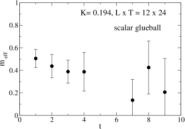
Figure 1: $m_{eff}$ of the $0^{++}$-glueball

Gluinoballs. The connected part of the correlation function was evaluated by choosing a random source, the disconnected by using the volume-source technique, both without smearing. The signal for the $a-\eta^{\prime}$ is reasonably good (see fig. 2) whereas for the $a-f_{0}$ no mass could be extracted yet.

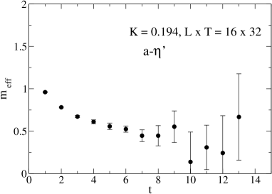
Figure 2: $m_{eff}$ of the $a-\eta^{\prime}$-gluinoball

Gluino-glueballs. The gluino-glue correlation $C^{\alpha\beta}(\Delta t)$ is evaluated by calculating the propagator $\Delta^{\alpha\beta}_{xy}$ for a random source $y$. APE as well as Jacobi smearing for the gluino have been used with parameters ($N_{APE}=9$, $\epsilon_{APE}=0.5$) and ($N_{Jac}=18$, $\epsilon_{Jac}=0.2$).

The pseudo chiral limit. Within the OZI-approximation the connected term in the $a-\eta^{\prime}$ correlator is expected to give rise to a massless mode in the limit $m_{\tilde{g}}\rightarrow 0$, the “adjoint pion” $a-\pi$ [6]. Extrapolating values for $m_{a-\pi}$ at various $\kappa$’s, we find $\kappa_{c}\simeq 0.1970(4)$, which is consistent with the determination in [2].

5 Conclusions and outlook

We still have work to do to fill out the blank spots in table 1. We plan to use better numerical technology such as variational smearing for glueballs, and stochastic estimators and spectral decomposition of the fermion propagator for the disconnected parts of the gluino-balls correlations. It would also be interesting to investigate the effects of the volume on the spectrum. For this better statistics are needed.

The computations were carried out on the Cray T3E at NIC, Jülich and the Sun Fire SMP-Cluster at RWTH Aachen, Germany.

References

- [1] I. Montvay, Int. J. Mod. Phys. A 17 (2002) 2377.
- [2] F. Farchioni et al. [DESY-Munster-Roma Collaboration], Eur. Phys. J. C 23 (2002) 719.
- [3] G. R. Farrar, G. Gabadadze and M. Schwetz, Phys. Rev. D 58 (1998) 015009.
- [4] I. Montvay, Nucl. Phys. B 466 (1996) 259.
- [5] I. Campos et al. [DESY-Munster Collaboration], Eur. Phys. J. C 11 (1999) 507.
- [6] G. Veneziano and S. Yankielowicz, Phys. Lett. B 113 (1982) 231.