An exact Polynomial Hybrid Monte Carlo algorithm for dynamical Kogut-Susskind fermions

Abstract

We present a polynomial Hybrid Monte Carlo (PHMC) algorithm as an exact simulation algorithm with dynamical Kogut-Susskind fermions. The algorithm uses a Hermitian polynomial approximation for the fractional power of the KS fermion matrix. The systematic error from the polynomial approximation is removed by the Kennedy-Kuti noisy Metropolis test so that the algorithm becomes exact at a finite molecular dynamics step size. We performed numerical tests with $N_{f}$$=$$2$ case on several lattice sizes. We found that the PHMC algorithm works on a moderately large lattice of $16^{4}$ at $\beta$$=$$5.7$, $m$$=$$0.02$ ($m_{\mathrm{PS}}/m_{\mathrm{V}}$$\sim$$0.69$) with a reasonable computational time.

1 Introduction

The low energy QCD dynamics in the real world will be understood by lattice QCD with three-flavors of dynamical quarks. Several efforts have been spent to develop exact numerical algorithms with an odd-numbers of the Wilson type quarks [1].

The Kogut-Susskind (KS) fermion is an attractive formalism since the numerical simulation with much lighter quark masses are possible thanks to the remnant chiral symmetry. Although lattice QCD with the two- or single-flavor KS fermions can be defined by taking the fractional power of the KS fermion, efficient exact algorithms are not still known. Approximate algorithms such as the $R$-algorithm [2] have been used in these cases.

Several exact algorithms are proposed for two- or single-flavor dynamical KS fermions [3, 4]. In this paper, we further study the idea by Horváth et al. [3] in the case of the polynomial Hybrid Monte Carlo (PHMC) algorithm. We develop two types of the PHMC algorithm depending on the choice of the effective action derived through the polynomial approximation. We compare the computational cost of these two PHMC algorithms. We investigate the property of the algorithm on several lattice sizes in $N_{f}$$=$$2$ case. We found that our algorithm shows satisfactory efficiency on a $16^{4}$ lattice with $\beta$$=$$5.7$, $m$$=$$0.02$ $(m_{\mathrm{PS}}/m_{\mathrm{V}}$$\sim$$0.69)$.

2 Algorithm

We construct two types of the PHMC algorithm, which are refereed to as case A and case B. Introducing a polynomial approximation and pseudo-fermion field, the partition function can be generally rewritten in the following form:

$$Z= \!\!\!\!\!\!\!\!\!\!\!\int{\cal D}U{\cal D}\phi_{o}^{{\dagger}}{\cal D}\phi_{o}\ \det[W^{(X)}[\hat{D}_{oo}]]^{N_{f}/4}$$ (1)

$$\ \ \ \ \ \ \ \ \ \ \ \ \ \ \ \ \times e^{-S_{g}[U]-S^{(X)}_{q}[U,\phi_{o}^{{\dagger}},\phi_{o}]},$$

where $S_{g}$ is a lattice gauge action, $\phi_{o}$ is pseudo-fermion field living only on odd sites. $S^{(X)}_{q}$ and $W^{(X)}$ are the pseudo-fermion action and the correction matrix respectively. The superscript $(X)$ takes $(A)$ or $(B)$ depending on the type of the PHMC algorithm as follows.

Case A: We approximate $\hat{D}_{oo}^{-N_{f}/8}$ by a $N_{\mathit{poly}}^{(A)}$ order polynomial $P_{N_{\mathit{poly}}^{(A)}}[\hat{D}_{oo}]$. The pseudo-fermion action and the correction term become

$$S^{(A)}_{q}[U,\phi_{o}^{{\dagger}},\phi_{o}] = |P_{N_{\mathit{poly}}^{(A)}}[\hat{D}_{oo}]\phi_{o}|^{2},$$

$$W^{(A)}[\hat{D}_{oo}] = \hat{D}_{oo}(P_{N_{\mathit{poly}}^{(A)}}[\hat{D}_{oo}])^{8/N_{f}}.$$ (2)

Case B: We approximate $\hat{D}_{oo}^{-N_{f}/4}$ by an even-order $N_{\mathit{poly}}^{(B)}$ polynomial $P_{N_{\mathit{poly}}^{(B)}}[\hat{D}_{oo}]$. The pseudo-fermion action and the correction term can be written as

$$S^{(B)}_{q}[U,\phi_{o}^{{\dagger}},\phi_{o}] = |Q_{N_{\mathit{poly}}^{(B)}}[\hat{D}_{oo}]\phi_{o}|^{2},$$

$$W^{(B)}[\hat{D}_{oo}] = \hat{D}_{oo}(P_{N_{\mathit{poly}}^{(B)}}[\hat{D}_{oo}])^{4/N_{f}},$$ (3)

where $Q_{N_{\mathit{poly}}^{(B)}}$ is the $N_{\mathit{poly}}^{(B)}/2$ order polynomial defined by $P_{N_{\mathit{poly}}^{(B)}}[\hat{D}_{oo}]$$=$$|Q_{N_{\mathit{poly}}^{(B)}}[\hat{D}_{oo}]|^{2}$.

The KS-fermion operator $\hat{D}_{oo}$ is even-odd preconditioned as $\hat{D}_{oo}$$=$$\mathbf{1}_{oo}$$-$$\lambda^{2}\hat{M}_{oo}$ with $\lambda^{2}$$=$$2\Lambda_{\mathrm{max}}$$/$ $(4m^{2}$$+$$2\Lambda_{\mathrm{max}}^{2})$ and $\hat{M}_{oo}$$=$$2M_{oe}M_{eo}/\Lambda_{\mathrm{max}}^{2}$$+$$\mathbf{1}_{oo}$. $\Lambda_{\mathrm{max}}$ is chosen so that the all eigenvalues of $\hat{M}_{oo}$ fall into the region $[-1,1]$. $M_{oe}$ ($M_{eo}$) is the usual KS hopping matrix from even (odd) to odd (even) sites.

For both cases, the algorithm takes the following two steps; (i) perform the HMC algorithm according to the effective action Eq. (2) or (3), (ii) when the HMC Metropolis test is accepted, apply the Kennedy-Kuti noisy Metropolis test to incorporate the correction term $W^{(X)}[\hat{D}_{oo}]]^{N_{f}/4}$. Thus we obtain two types of the PHMC algorithm depending on the choice of the effective action.

The acceptance probability of the noisy-Metropolis test is defined by

$$P_{\mathrm{NMP}}[U\rightarrow U^{\prime}]=\min[1,e^{-dS}],$$

$$dS=\zeta_{o}^{{\dagger}}W^{(X)}[\hat{D}_{oo}^{\prime}]^{-N_{f}/4}\zeta_{o}-|\eta_{o}|^{2},$$ (4)

where $\zeta_{o}$$=$$W^{(X)}[\hat{D}_{oo}]^{N_{f}/8}\eta_{o}$ with a Gaussian noise vector $\eta_{o}$. $W^{(X)}[\hat{D}_{oo}]$ is calculated on an initial configuration and $W^{(X)}[\hat{D}_{oo}^{\prime}]$ is on a trial configuration generated by the preceding HMC algorithm.

The fractional power of the correction matrix $W^{(X)}$ is taken by the Lanczos based Krylov subspace method proposed by Boriçi [6]. We modified his algorithm suitable to our purpose. As indicated by Boriçi we employ CG based stopping criterion for the Lanczos based method.

3 Cost estimate

The computational cost is counted as the number of multiplication of the hopping matrix to evolve the algorithm unit trajectory. We employ single leapfrog integration scheme for the molecular dynamics (MD) step. We roughly estimate it as

$$\!\!\!\!\!\!\!\!\!\!\!N_{\mathrm{CostA}}=(2N_{\mathit{poly}}^{(A)}-1)\times N^{(A)}_{\mathrm{MD}}$$

$$\ \ \ \ \ +3\times((8/N_{f})\times N_{\mathit{poly}}^{(A)}+1)\times N^{(A)}_{\mathrm{CG}},$$

$$\!\!\!\!\!\!\!\!\!\!\!N_{\mathrm{CostB}}=(N_{\mathit{poly}}^{(B)}-1)\times N^{(B)}_{\mathrm{MD}}$$

$$\ \ \ \ \ +3\times((4/N_{f})\times N_{\mathit{poly}}^{(B)}+1)\times N^{(B)}_{\mathrm{CG}},$$

where $N_{\mathrm{MD}}$ is the number of MD step and $N^{(X)}_{\mathrm{CG}}$ the number of iteration of CG algorithm. The CG algorithm is used to generate $\phi_{o}$ with the global heat-bath method and in the Lanczos based algorithm for the noisy Metropolis test.

Now we compare the costs by specifying $N_{\mathit{poly}}^{(A)}$ and $N_{\mathit{poly}}^{(B)}$. For this purpose we employ the Chebyshev polynomial approximation;

$$x^{-s}=(1+\lambda^{2}y)^{-s}\sim P_{N_{\mathit{poly}}}[x]=\sum_{i=0}^{N_{\mathit{poly}}}c_{k}T_{k}[y],$$ (5)

where $T_{k}$ is the $k$-th order Chebyshev polynomial, $x$$=$$\hat{D}_{oo}$ and $y$$=$$-\hat{M}_{oo}$ can be read of. The coefficients $c_{k}$ are calculated as usual.

Figure 1 shows the cost $N_{\mathit{poly}}/s$ dependence of the integrated residual defined by $\sqrt{R^{2}}$$=$$(\int_{-1}^{1}dy|x(P_{N_{\mathit{poly}}}[x])^{1/s}-1|^{2})^{1/2}$ for each $s$. We observe that as decreasing $s$ by factor $1/2$ the cost $N_{\mathit{poly}}/s$ increases by factor $2$ at a constant $\sqrt{R^{2}}$. This is nothing but $N_{\mathit{poly}}$ does not depend on the choice of $s$ and we obtain $N_{\mathit{poly}}^{(A)}$$\sim$$N_{\mathit{poly}}^{(B)}$ at a constant approximation level.

Using this relation and assuming $N_{\mathrm{CG}}^{(A)}$$=$$N_{\mathrm{CG}}^{(B)}$ and $N_{\mathrm{MD}}^{(A)}$$=$$N_{\mathrm{MD}}^{(B)}$, we find $N_{\mathrm{CostA}}$$\sim$$2N_{\mathrm{CostB}}$. We employ the Chebyshev polynomial and the plaquette gauge action, and apply the case B PHMC algorithm for numerical simulations.

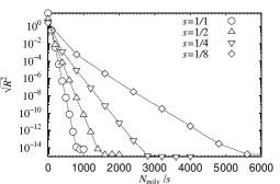
Figure 1: $N_{\mathit{poly}}/s$ dependence of the integrated residual $\sqrt{R^{2}}$ with $1-\lambda^{2}=1/1000$.

4 Results

Figure 2 shows the MD step size dependence of the averaged plaquette on a $8^{3}\times 4$ lattice at $\beta$$=$$5.26$ and $m$$=$$0.025$. The results with the PHMC algorithm of $N_{\mathit{poly}}$$=$$200$ do not depend on $dt$ as it should be and produce the consistent result to that in the zero MD step size limit of the $R$-algorithm. Although we do not show the results on the $N_{\mathit{poly}}$ dependence, the results are independent of the choice of $N_{\mathit{poly}}$.

In Table 1 we show the numerical results on a $16^{4}$ lattice at $\beta$$=$$5.7$ and $m$$=$$0.02$. The averaged plaquette are independent of $N_{\mathit{poly}}$ and consistent with each other as expected. On the other hand, the $R$-algorithm yields $\langle P\rangle$$=$$0.577261(49)$ [7], which differs from ours by $\sim$$2\sigma$. This indicates a potential systematic error for the $R$-algorithm at finite MD step size. The computational time for $N_{\mathit{poly}}$$=$$300$ with $m$$=$$0.02$ (which corresponds to $m_{\mathrm{PS}}/m_{\mathrm{V}}$$\sim$$0.69$ [7]) was measured as 112 sec. to achieve unit trajectory with 14 GFlops sustained speed of SR8000 at KEK.

Figure 2: MD step size $dt$$=$$1/N_{\mathrm{MD}}$ dependence of the averaged plaquette $\langle P\rangle$ on the small size lattice. $N_{\mathit{poly}}$$=$$200$, $N_{\mathrm{MD}}$$=$$25$, and $\Lambda_{\mathrm{max}}$$=$$2.37$ are employed for the PHMC.

Table 1: Numerical results on a $16^{4}$ lattice at $\beta$$=$$5.7$ and $m$$=$$0.02$. $\Lambda_{\mathrm{max}}$$=$ $2.28$ is employed.

$N_{\mathrm{poly}}$	300	400	500
$[dt,N_{\mathrm{MD}}]$	$[0.02,50]$	$[0.02,50]$	$[0.02,50]$
Traj.	1700	1050	800
$\langle P\rangle$	0.577099(46)	0.577130(46)	0.577023(43)

Consequently we conclude that the PHMC algorithm we constructed works on a moderately large lattice size with rather heavy quark masses with reasonable computational cost. The algorithm also works with a single-flavor fermion. We emphasize that because the PHMC algorithm is exact one, it must be a promising algorithm for future realistic simulations.

This work is supported by the Supercomputer Project No. 79 (FY2002) of High Energy Accelerator Research Organization (KEK), and also in part by the Grant-in-Aid of the Ministry of Education (Nos. 11640294, 12304011, 12740133, 13135204, 13640259, 13640260). N.Y. is supported by the JSPS Research Fellowship.

References

[1]
T. Takaishi and Ph. de Forcrand,
Int. J. Mod. Phys. C13 (2002) 343;
Nucl. Phys. (Proc. Suppl.) 94 (2001) 818;
hep-lat/0009024;
JLQCD collaboration,
S. Aoki et al., Phys. Rev. D 65 (2002) 094507;
F. Farchioni, C. Gebert, I. Montvay, and W. Schroers,
Nucl.Phys.Proc.Suppl. 106 (2002) 215.
[2]
M. Clark, in these proceedings.
[3]
I. Horváth, A. D. Kennedy, and S. Sint,
Nucl. Phys. B (Proc. Suppl.) 73 (1999) 834.
[4]
A. Hasenfratz and F. Knechtli,
hep-lat/0106014; Nucl. Phys. B (Proc. Suppl.) 106 (2002);
hep-lat/0203010; in these proceedings.
[5]
A. D. Kennedy and J. Kuti,
Phys. Rev. Lett. 54 (1985) 2473.
[6]
A. Boriçi,
Phys. Lett. B453 (1999) 46;
J. Comput. Phys. 162 (2000) 123;
hep-lat/0001019.
[7]
M. Fukugita et al.,
Phys. Rev. D 47 (1993) 4739.