Chiral symmetry breaking in (2+1) dimensional QED

Abstract

We study dynamical mass generation in QED in (2+1) dimensions using Hamiltonian lattice methods. We use staggered fermions, and perform simulations with explicit dynamical fermions in the chiral limit. We demonstrate that a recently developed method to reduce the fermion sign problem can successfully be applied to this problem. Our results are in agreement with both the strong coupling expansion and with Euclidean lattice simulations.

1 INTRODUCTION

QED in (2+1) dimensions exhibits both dynamical mass generation [1, 2, 3, 4, 5] and confinement [6]. This makes it an interesting theory to study these nonperturbative phenomena. Furthermore, these phenomena in QED₃ are relevant for applications in condensed matter physics, in particular in connection with high-$T_{c}$ superconductivity [7]. Here, we focus on the question of chiral symmetry breaking in QED₃.

We use staggered fermions, and perform simulations with explicit dynamical fermions in the chiral limit. Simulations with explicit fermions could improve our understanding of the microscopic behavior of (chiral) fermions in lattice simulations. We apply a recently developed method [8], called the “zone method”, to reduce the fermion sign problem in our simulation. Preliminary results for the chiral condensate in QED₃ are in agreement with other methods.

2 QED IN (2+1) DIMENSIONS

QED₃ is a superrenormalizable theory, with a dimensionful coupling: $e^{2}$ has dimensions of mass. This dimensionful parameter plays a role similar to $\Lambda_{\rm QCD}$ in QCD. In the chiral limit, it sets the energy scale.

We use 4-component spinors, such that the fermion mass term is even under parity. With one massless fermion, the Hamiltonian exhibits a global $U(2)$ “chiral” symmetry. A fermion mass term breaks this symmetry to a $U(1)\times U(1)$ symmetry. The question is: is this chiral symmetry broken dynamically? The order parameter for this symmetry breaking is the chiral condensate.

There are extensive studies using the Dyson–Schwinger equations [2] suggesting that there is dynamical chiral symmetry breaking in QED₃ if the number of fermion flavors is smaller than some critical number $N_{c}\sim 3.3$. However, the scale of this symmetry breaking (i.e. the magnitude of the condensate) is rather small.

2.1 Hamiltonian Lattice Simulations

Following the notation of Ref. [4], we consider the lattice Hamiltonian in (2+1) dimensions

$$H = \frac{g^{2}}{2a}(W_{0}+yW_{1}+y^{2}W_{2})\;,$$ (1)

with

$$W_{0} = \sum_{l}E_{l}^{2}-\mu\sum_{\vec{r}}(-1)^{r_{1}+r_{2}}\chi^{\dagger}(\vec{r})\chi(\vec{r})\;,$$ (2)

$$W_{1} = \sum_{\vec{r},j}\eta_{j}(\vec{r})\chi^{\dagger}(\vec{r})U_{j}(\vec{r})\chi(\vec{r}+\hat{j})+{\rm h.c.}\;,$$ (3)

$$W_{2} = -\sum_{p}\left(U_{p}+U^{\dagger}_{p}\right)\;.$$ (4)

where $\eta_{1}(\vec{r})=(-1)^{r_{2}+1}$, $\eta_{2}(\vec{r})=1$, $y=1/g^{2}$, and $U_{p}$ is the usual plaquette operator. We use a dimensionless mass parameter $\mu=2m/e^{2}$ and a dimensionless coupling constant $g^{2}=e^{2}a$ where $a$ is the lattice spacing. The continuum limit corresponds to $y\to\infty$ or $g^{2}\to 0$.

We use staggered fermions, corresponding to one 4-component fermion flavor in the continuum limit [4, 9]. For $\mu=0$, the lattice breaks the “chiral” $U(2)$ symmetry to a discrete symmetry generated by a shift of one lattice spacing. A nonzero mass term breaks this discrete symmetry. To study chiral symmetry breaking on the lattice, we calculate the lattice condensate $\langle\bar{\psi}\psi\rangle$ in the chiral limit as function of the lattice coupling $y$. It is related to the continuum condensate

$$y^{2}\langle\bar{\psi}\psi\rangle^{\hbox{\scriptsize lattice}} = \frac{1}{e^{4}}\langle\bar{\psi}\psi\rangle^{\hbox{\scriptsize continuum}}\;,$$ (5)

in the limit $y\rightarrow\infty$.

We use a finite spatial grid, $N_{1}\times N_{2}$, and calculate observables

$$\langle{\cal O}\rangle = \frac{\langle\Psi_{\hbox{\scriptsize final}}|{\rm e}^{\frac{-HT}{2}}{\cal O}{\rm e}^{\frac{-Ht}{2}}|\Psi_{\hbox{\scriptsize initial}}\rangle}{\langle\Psi_{\hbox{\scriptsize final}}|{\rm e}^{-Ht}|\Psi_{\hbox{\scriptsize initial}}\rangle}\;,$$ (6)

by dividing the Euclidean time variable $t$ in $N_{t}$ slices, and inserting a complete set of states between the time slices. We choose a tensor product basis of gauge and fermion states. We use a standard Metropolis algorithm to update the gauge field configurations.

For the fermions we use the worldline formalism [10], in combination with the loop algorithm [11] to update the fermion configurations. As initial/final states we choose the strong coupling ($y\to 0$) ground state. The initial and final fermion states are identical, up to permutations of fermions. Numerically, these permutations of course give rise to the fermion sign problem. With the worldline formalism we can keep track of the permutations, and we use the newly developed zone method [8] to reduce the sign problem.

2.2 Zone method

The basic idea [8] is to introduce an $n_{1}\times n_{2}$ spatial sub-lattice (with $n_{i}\leq N_{i}$), which we call a zone, for the fermion simulations, see Fig. 1. Next, we allow for permutations of initial and final state fermions inside this zone only.

Figure 1: Illustration of the zone method: an $6\times 8$ spatial lattice with a $3\times 4$ zone. The size of this zone is 17, as characterized by the number of links inside the sub-lattice.

We do not allow for any configuration with fermion permutations outside the $n_{1}\times n_{2}$ spatial sub-lattice. Note that at intermediate time slices the fermions are still allowed to wander through the entire $N_{1}\times N_{2}$ lattice. In order to further reduce the fermion sign problem, we also use a larger value of the coupling $y^{\prime}$ and a larger value of the fermion mass $m^{\prime}$ when the fermions are outside this zone.

It turns out that observables scale linearly in the zone size, provided that this zone size is larger than the characteristic “fermion wandering length” [8]. For any finite values of the coupling $y$ and of the time variable $t$, this wandering length is finite, even for massless fermions. Thus one can extrapolate the results from relatively small zones to the entire lattice.

3 NUMERICAL RESULTS

There are different ways to define the size of a zone: by number of lattice points or by the number of links inside the zone. For large lattices it does not matter which one one chooses. However, for the relatively small lattices we have used sofar, it turns out that the best way to characterize the zone size is the number of links inside the zone.

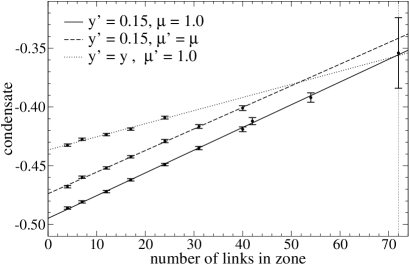
Figure 2: Numerical results for different zone sizes within a $6\times 6$ lattice, for fixed values of $y=0.5$, $\mu=0$, $t=1.5$, and $N_{t}=10$. The total number of links in the lattice is 72, where the three linear fits meet (within error bars).

In Fig. 2 we show that, within error bars, the chiral condensate indeed behaves linearly in the number of links inside the fermion zone, even for the smallest zones (at least for these parameter values). Thus we can use a linear extrapolation to obtain the lattice condensate for the entire lattice, using three or four different zone sizes.

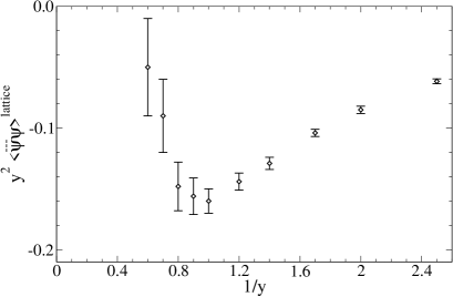
Figure 3: Our results for the lattice condensate as function of $y$, obtained by extrapolating several different zone sizes for a finite value of $t$.

In Fig. 3 we show our results for a range of values of the coupling $y$. These results are obtained on lattices up to $8\times 8$ using several different zone sizes and for finite values of $t$. The error bars are statistical error bars only. We expect the finite size effects due to the spatial lattice to be smaller than these error bars; however, preliminary results indicate the $t=\infty$ extrapolation could lead to a reduction by about 10%. We are currently working on estimating the finite size effects in more detail [12].

For $y<1$ these results agree quite well with the strong coupling expansion [4], whereas the strong decrease with increasing $y$ for $1<y<2$ is in good agreement with Euclidean Monte Carlo simulations [3]. It is unclear yet whether or not the condensate obtained this way is small or exactly zero in the continuum limit, $y\to\infty$.

References

- [1] R. D. Pisarski, Phys. Rev. D 29, 2423 (1984).
- [2] T. W. Appelquist, M. J. Bowick, D. Karabali and L. C. Wijewardhana, Phys. Rev. D 33, 3704 (1986); P. Maris, Phys. Rev. D 54, 4049 (1996).
- [3] A. N. Burkitt and A. C. Irving, Nucl. Phys. B 295, 525 (1988).
- [4] C. J. Hamer, J. Oitmaa and W. h. Zheng, Phys. Rev. D 57, 2523 (1998).
- [5] S. J. Hands, J. B. Kogut and C. G. Strouthos, arXiv:hep-lat/0208030.
- [6] C. J. Burden, J. Praschifka and C. D. Roberts, Phys. Rev. D 46, 2695 (1992); P. Maris, Phys. Rev. D 52, 6087 (1995); G. Grignani, G. W. Semenoff and P. Sodano, Phys. Rev. D 53, 7157 (1996); M. N. Chernodub, E. M. Ilgenfritz and A. Schiller, arXiv:hep-lat/0208013.
- [7] M. Franz and Z. Tesanovic, Phys. Rev. Lett. bf 87, 257003 (2001); M. Franz, Z. Tesanovic, and O. Vafek, Phys. Rev. B 65, 180511 (2002); ibid., Phys. Rev. B 66, 054535 (2002); Igor F. Herbut, Phys. Rev. Lett. 88, 047006 (2002); ibid., arXiv:cond-mat/0202491.
- [8] Dean Lee, arXiv:cond-mat/0202283; ibid., arXiv:hep-lat/0209047, these proceedings.
- [9] C. J. Burden and C. J. Hamer, Phys. Rev. D 37, 479 (1988).
- [10] J. E. Hirsch, D. J. Scalapino, R. L. Sugar, and R. Blankenbecler, Phys. Rev. Lett. 47, 1628 (1981); ibid., Phys. Rev. B 26, 5033 (1982).
- [11] H. G. Evertz, G. Lana, and M. Marcu Phys. Rev. Lett. 70, 875 (1993); H. G. Evertz, arXiv:cond-mat/9707221.
- [12] Dean Lee and Pieter Maris, in preparation.