Zone methods and the fermion sign problem

Abstract

We review a recently proposed approach to the problem of alternating signs for fermionic many body Monte Carlo simulations in finite temperature simulations. We derive an estimate for fermion wandering lengths and introduce the notion of permutation zones, special regions of the lattice where identical fermions may interchange and outside of which they may not. Using successively larger permutation zones, one can extrapolate to obtain thermodynamic observables in regimes where direct simulation is impossible.

1 Introduction

The zone method approach to the fermion sign problem is based on the observation that in many finite temperature simulations fermion permutations are short ranged [1]. This can be true even for systems with massless modes and long distance correlations, as we demonstrate with an explicit example. In this proceedings article we derive an estimate for the finite temperature fermion wandering length and discuss the main features of the zone method.

2 Worldlines

We begin with a brief review of the worldline formalism [2].  We introduce ideas in one spatial dimension before moving on to higher dimensions.  Let us consider a system with one species of fermion on a periodic chain with $L$ sites, where $L$ is even.  Aside from an additive constant, the general Hamiltonian can be written as

$$H=-h\sum_{i}\left[a_{i+1}^{\dagger}a_{i}+a_{i}^{\dagger}a_{i+1}\right]+\sum_{i}c_{i}a_{i}^{\dagger}a_{i}.$$ (1)

Following [2] we break the Hamiltonian into two parts, $H_{\text{e}}$ and $H_{\text{o}}$,

$$H_{\text{e/o}}=\sum_{i\text{ even/odd}}\left[\begin{array}[]{c}-ha_{i+1}^{\dagger}a_{i}-ha_{i}^{\dagger}a_{i+1}\\ +{\textstyle{c_{i}\over 2}}a_{i}^{\dagger}a_{i}+{\textstyle{c_{i+1}\over 2}}a_{i+1}^{\dagger}a_{i+1}\end{array}\right].$$

We note that $H=H_{\text{e}}+H_{\text{o}}$. For large $N$, we can write

$$\exp(-\beta H)\approx(S_{\text{o}}S_{\text{e}})^{N},$$ (2)

where

$$S_{\text{e/o}}=\exp(-{\textstyle{\beta\over N}}H_{\text{e/o}}).$$ (3)

Inserting a complete set of states at each step, we can write $Tr\left[\exp(-\beta H)\right]$ as

$$\sum_{z_{0},...,z_{2N-1}}\left\langle z_{0}\right|S_{\text{o}}\left|z_{2N-1}\right\rangle...\left\langle z_{1}\right|S_{\text{e}}\left|z_{0}\right\rangle.$$ (4)

The worldline trajectory of each of the fermions can now be traced from Euclidean time $t=0$ to time $t=\beta$. Since we are computing a thermal trace, the worldlines from $t=0$ to $t=\beta$ define a permutation of identical fermions.  Even permutations carry a fermion sign of $+1$ while odd permutations carry sign $-1$. The generalization to higher dimensions is straightforward. In two dimensions, for example, $\exp(-\beta H)$ takes the form

$$\left.\begin{array}[]{c}\left[\exp\left[-{\textstyle{\beta\over N}}(H_{\text{e}}^{x}+H_{\text{o}}^{x}+H_{\text{e}}^{y}+H_{\text{o}}^{y})\right]\right]^{N}\\ \qquad\qquad\qquad\approx(S_{\text{o}}^{y}S_{\text{e}}^{y}S_{\text{o}}^{x}S_{\text{e}}^{x})^{N}.\end{array}\right.$$ (5)

3 Wandering length

In one spatial dimension, the Pauli exclusion principle inhibits fermion permutations except in cases where the fermions wrap around the lattice boundary.  For the remainder of our discussion, therefore, we consider systems with two or more dimensions.  The first question we address is how far fermion worldlines can wander from start time $t=0$ to end time $t=\beta$.  We can put an upper bound on this wandering distance by considering the special case with no on-site potential and only nearest neighbor hopping.

Let us consider motion in the $x$-direction.  For each factor of $S_{\text{o}}^{x}S_{\text{e}}^{x}$ in (5) a given fermion may remain at the same $x$ value, move one lattice space to the left, or move one lattice space to the right.  If $h$ is the hopping parameter, then for large $N$ the relative weights for these possibilities are approximately $1$ for remaining at the same $x$ value, $\beta hN^{-1}$ for one move to the left, and $\beta hN^{-1}$ for one move to the right.  In (5) we see that there are $N$ factors of $S_{\text{o}}^{x}S_{\text{e}}^{x}$.  Therefore for a typical worldline configuration at low filling fraction, $f,$ we expect $\sim\beta h$ hops to the left and $\sim\beta h$ hops to the right.  For non-negligible $f$ some of the hops are forbidden by the exclusion principle.  Assuming random filling we expect $\sim(1-f)\beta h$ hops to the left and $\sim(1-f)\beta h$ hops to the right.

The net displacement is equivalent to a random walk with $2(1-f)\beta h$ steps.  The expected wandering length, $\Delta,$ is therefore given by

$$\Delta=\sqrt{2(1-f)\beta h}.$$ (6)

In cases with on-site potentials, fermion hopping is dampened by differences in potential energy.  Hence the estimate (6) serves as an upper bound for the general case.  We have checked the upper bound numerically using simulation data generated by many different lattice Hamiltonians with and without on-site potentials.

4 Permutation Zone Method

Let $W$ be the logarithm of the partition function,

$$W=\log\left\{Tr\left[\exp(-\beta H)\right]\right\}.$$ (7)

Let us partition the spatial lattice, $\Gamma$, into zones $Z_{1},Z_{2},...,Z_{k}$ such that the spatial dimensions of each zone are much greater than $\Delta$.  For notational convenience we define $Z_{0}=\emptyset$.  For any $R\subset\Gamma$, let $W_{R}$ be the logarithm of a restricted partition function that includes only worldline configurations such that any worldline starting at $t=0$ outside of $R$ returns to the same point at $t=\beta$.  In other words there are no permutations for worldlines starting outside of $R$.  We note that $W_{\Gamma}=W,$ and $W_{\emptyset}$ is the logarithm of the restricted partition function with no worldline permutations at all.  Since the zones are much larger than the length scale $\Delta$, the worldline permutations in one zone has little or no effect on the worldline permutations in another zones.  Therefore

$$W_{Z_{0}\cup...Z_{j}}-W_{Z_{0}\cup...Z_{j-1}}\approx W_{Z_{j}}-W_{\emptyset}.$$ (8)

Using a telescoping series, we obtain

$$W_{\Gamma}-W_{\emptyset}=\sum_{j=1,...,k}(W_{Z_{0}\cup...Z_{j}}-W_{Z_{0}\cup...Z_{j-1}}),$$ (9)

$$W_{\Gamma}-W_{\emptyset}\approx\sum_{j=1,...,k}(W_{Z_{j}}-W_{\emptyset}).$$ (10)

For translationally invariant systems tiled with congruent zones we find

$$W=W_{\Gamma}\approx W_{\emptyset}+{\textstyle{\left|\Gamma\right|\over\left|Z_{1}\right|}}(W_{Z_{1}}-W_{\emptyset}),$$ (11)

where $\left|\Gamma\right|/\left|Z_{1}\right|\equiv k$, the number of zones.  For general zone shapes one can imagine partitioning the zones themselves into smaller congruent tiles.  Therefore the result (10) should hold for large arbitrarily shaped zones.  For this case we take $\left|\Gamma\right|$ to be the number of nearest neighbor bonds in the entire lattice and $\left|Z_{1}\right|$ to be the number of nearest neighbor bonds in the zone.  We will refer to $\left|Z_{1}\right|$ as the zone size of $Z_{1}$.  This is just one choice for zone extrapolation.  A more precise and complicated scheme could be devised which takes into account the circumscribed volume, number of included lattice points, and other geometric quantities.

As an example of the permutation zone method, we compute the average energy $\left\langle E\right\rangle h^{-1}$ for a free fermion Hamiltonian with only hopping on an $8\times 8$ lattice.  We set the number of time steps $N=8$ and consider values $\beta h=1.0$, $1.5$, and $2.0$.  The corresponding values for $\Delta$ are $1.0$, $1.2$, and $1.4$ respectively.  The Monte Carlo updates were performed using our own version of the single-cluster loop algorithm [3]. In Figure 1 we show data for rectangular zones with side dimensions $0\times 0$, $1\times 1$, $2\times 1$, $2\times 2$, $3\times 2$, $3\times 3$, …, $6\times 6$.  We also show a least-squares fit (not including the smallest zones $0\times 0$ and $1\times 1$) assuming linear dependence on zone size as predicted in (10).  We find agreement at the $1\%$ level or better when compared with the exact answers shown on the far right, which were computed using momentum-space decomposition.

While the physics of the free hopping Hamiltonian is trivial, the computational problems are in fact maximally difficult.  The severity of the sign problem can be measured in terms of the average sign, $<$Sign$>$, for contributions to the partition function.  For $\beta h=1.0$, $<$Sign$>\sim 0.005;$ for $\beta h=1.5$, $<$Sign$>$ $\sim 10^{-6};$ and for $\beta h=2.0$, $<$Sign$>$$\sim 10^{-9}$.  Direct calculation using position-space Monte Carlo is impossible by several orders of magnitude for $\beta h\geq 1.5$.

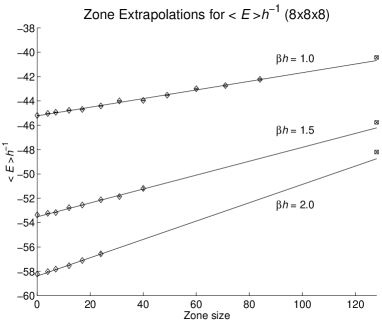
Figure 1: Average energy at $\beta h=1.0,1.5,2.0$ for the free fermion Hamiltonian on an $8\times 8$ lattice.

5 Summary

We have reviewed the zone method approach to the fermion sign problem. We have demonstrated that the exchange of identical fermions is short-ranged and has a maximum range of $\sqrt{2(1-f)\beta h}$ lattice sites, where $\beta$ is the inverse temperature, $h$ is the hopping parameter, and $f$ is the filling fraction. We have introduced the notion of permutation zones, special regions of the lattice where identical fermions may interchange and outside of which they may not. Using successively larger permutation zones, one can extrapolate to obtain thermodynamic observables. Applications of the zone method to chiral symmetry breaking in (2+1) dimensional QED is discussed in another article in these proceedings [4].

References

- [1] D. Lee, cond-mat/0202283.
- [2] J. Hirsch, D. Scalapino, R. Sugar, R. Blankenbecler, Phys. Rev. Lett. 47 1628 (1981); Phys. Rev. B 26 5033 (1982).
- [3] H. G. Evertz, to appear in Numerical Methods of Lattice Quantum Many-Body Problems, edited by D. J. Scalapino, Perseus, Berlin, 2001; H. G. Evertz, G. Lana, M. Marcu, Phys. Rev. Lett. 70, 875 (1993); H. G. Evertz, M. Marcu in Quantum Monte Carlo Methods in Condensed Matter Physics, p. 65, edited by M. Suzuki, World Scientific, 1994.
- [4] P. Maris, D. Lee, these proceedings.