Multiple molecular dynamics time-scales in Hybrid Monte Carlo fermion simulations.

Abstract

A scheme for separating the high- and low-frequency molecular dynamics modes in Hybrid Monte Carlo (HMC) simulations of gauge theories with dynamical fermions is presented. The algorithm is tested in the Schwinger model with Wilson fermions.

At this conference, much discussion focussed on the dominant systematic error facing dynamical fermion simulations; the chiral extrapolation. It is proving to be a significant challenge to run Wilson fermion simulations of QCD using the HMC algorithm at light quark masses [1].

The standard implementation of HMC introduces pseudofermion fields to mimic the fermion action, and generates new proposals to a Metropolis test by integrating the molecular-dynamics (MD) equations of motion for a Hamiltonian in a fictitious simulation time. The maximum step-size for a useful Metropolis acceptance rate is set by a characteristic time-scale of the action used in the Hamiltonian [2]. Recent studies find that as the fermion is made lighter, the force induced by the pseudofermions generates increasingly violent high-frequency fluctuations. This effect is called “ultra-violet slowing-down” in Ref. [3]. In this report, we describe a modification to HMC that attempts to address this problem. A number of interesting algorithms have been devised recently that reduce the influence of the UV fermion modes on either the Monte Carlo update scheme or in the lattice discretisation [3, 4, 5, 6, 7].

1 MULTIPLE MD TIME-SCALES

A scheme for integrating the equations of motion for the MD phase of the HMC algorithm by introducing different time-scales for different segments of the action was introduced in Ref. [8].

The leap-frog integrator is constructed from the two simple time-evolution operators generated by the the kinetic and potential energy terms. Their effect on the system coordinates, $\{p,q\}$ are

$$V_{T}(\Delta\tau):\{p,q\} \longrightarrow \{p,q+\Delta\tau\;p\}$$

$$V_{S}(\Delta\tau):\{p,q\} \longrightarrow \{p-\Delta\tau\;\partial S,q\}$$ (1)

The simplest reversible leap-frog integrator is then

$$V(\Delta\tau)=V_{S}(\frac{\Delta\tau}{2})V_{T}(\Delta\tau)V_{S}(\frac{\Delta\tau}{2}).$$ (2)

If the action (and thus the Hamiltonian) is split into two parts,

$${\cal H}=\underbrace{T(p)+S_{1}(q)}_{{\cal H}_{1}}+\underbrace{S_{2}(q)}_{{\cal H}_{2}},$$ (3)

then the two leap-frog integrators for these two pieces can be constructed as

$$V_{1}(\Delta\tau) = V_{S_{1}}(\frac{\Delta\tau}{2})\;V_{T}(\Delta\tau)\;V_{S_{1}}(\frac{\Delta\tau}{2})$$

$$V_{2}(\Delta\tau) = V_{S_{2}}(\Delta\tau)$$ (4)

and a reversible integrator for the full Hamiltonian can be constructed by combining the two schemes:

$$V(\Delta\tau)=V_{2}(\frac{\Delta\tau}{2})\;\left[V_{1}(\frac{\Delta\tau}{m})\right]^{m}\;V_{2}(\frac{\Delta\tau}{2}),$$ (5)

with $m\in Z$. This compound integrator effectively introduces two evolution time-scales, $\Delta\tau$ and $\Delta\tau/m$.

We suggest that the multiple time-scale scheme is only helpful when two criteria are fulfilled simultaneously:

1. the force term generated by $S_{1}$ is cheap to compute compared to that of $S_{2}$ and

2. the split captures the high-frequency modes of the system in $S_{1}$ and the low-frequency modes in $S_{2}$.

The popular implementation of the scheme in dynamical fermion simulations with pseudofermions is to split the Hamiltonian into the Yang-Mills term and the pseudofermion action:

$$S_{1} = S_{G},$$

$$S_{2} = \phi^{*}[M^{\dagger}M]^{-1}\phi$$ (6)

Unfortunately for light fermions, the highest frequency fluctuations are in the pseudofermion action, which also has the more computationally expensive force term, thus the criteria are not met. The key to using the method then is to implement a low-computational cost scheme that separates the high- and low-frequency fermion molecular-dynamics.

2 POLYNOMIAL FILTERING

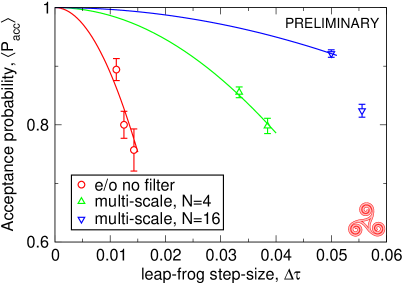
Figure 1: The HMC acceptance rate as a function of MD step-size for the standard leap-frog method, and for the new algorithm with $N=4$ and $16$

A very low-order polynomial approximation offers a cheap means of mimicking most of the short-distance physics of the fermion interations. Recent interest in polynomial approximations to a matrix inverse was inspired by the multi-boson algorithm of Ref. [10]. This led to the development of the Polynomial HMC (PHMC) algorithm [11]. Following this idea, we write an exact representation of the two-flavour probability measure

$$\det M^{\dagger}M=\int\!\!{\cal D}\phi{\cal D}\phi^{*}{\cal D}\chi{\cal D}\chi^{*}e^{\left\{-S_{\phi}-S_{\chi}\right\}}$$ (7)

with

$$S_{\phi}=\left|[M{\cal P}(M)]^{-1}\phi\right|^{2}\mbox{ and }S_{\chi}=\left|{\cal P}(M)\chi\right|^{2}$$ (8)

The fields $\phi$ are modified pseudofermions and we term the new fields $\chi$, “guide” bosons. The algorithm exactly recovers the probability measure for the two-flavour theory for any choice of polynomial. This scheme is similar to the split-pseudofermion method of Ref. [9] with one distinction; using polynomials allows us to modify the fermion modes easily and cheaply. The success of the algorithm hinges on the empirical observation that the fermion modes that induce the high-frequency fluctuations are localised and can be handled by very low-order polynomials. This means the force term for the guide bosons, generated by $S_{\chi}$ can be computed cheaply and a multiple time-scale integrator can be built that simultaneously fulfills the two criteria discussed earlier. The time-scale split is then

$$S=\underbrace{S_{G}+S_{\chi}}_{UV,\;\;\partial S\mbox{ cheap}}+\underbrace{S_{\phi}}_{IR,\;\;\partial S\mbox{ costly.}}$$ (9)

Note that in general, $p$ time-scales can be introduced straightforwardly by first adding $p-1$ sets of guide fields, then constructing a heirarchy of leapfrog integrators, with $m_{i}$ leap-frog steps at the $i^{\rm th}$ level. This introduces $p$ time-scales, $\Delta\tau>\frac{\Delta\tau}{m_{p-1}}\dots\frac{\Delta\tau}{m_{p-1}\dots m_{1}}$.

3 TESTING THE ALGORITHM

The performance of the method is under investigation in simulations of the two-flavour massive Schwinger model ($2d$ QED). HMC runs presented here are performed on $64\times 64$ lattices, with $\beta=4.0,\kappa=0.2618$. Non-hermitian Chebyshev polynomial approximations are used [12]. Measurements of the dependence of the acceptance probability on the polynomial degree and tuning the MD parameters, $\Delta\tau$ and $m$ are being made.

Fig. 1 shows the acceptance rate for the standard HMC algorithm (with even-odd preconditioned pseudofermions) along with the polynomial-filtered method. Two different polynomials were used; $N=4$ and $N=16$. The solid lines are fits to the expected behaviour of HMC as $\Delta\tau\rightarrow 0$, namely

$$\langle P_{\rm acc}\rangle=\mbox{erfc}\left\{(\Delta\tau/\tau_{0})^{2}\right\},$$ (10)

where the value of $\tau_{0}$ is determined by the best fit. $\tau_{0}$ is then a characteristic time-scale for the modes encapsulated in the pseudofermionic part of the action, $S_{\phi}$ in Eqn. 8. Since evaluation of the force term $\partial S_{\phi}$ dominates in this parameter range, $\tau_{0}$ is a good indicator of algorithm performance.

4 TUNING THE ALGORITHM

The algorithm has a number of free parameters, allowing a good deal of scope to optimise the performance. Fig. 2 shows the characteristic time-scale for pseudofermion integration, $\tau_{0}$ as a function of Chebyshev polynomial degree. $\tau_{0}$ rises very rapidly initially as the degree of the filter algorithm is increased, and $\tau_{0}$ for $N=16$ is about four times larger than for the standard HMC algorithm. Inverting the pseudofermion matrix requires roughly the same computational cost, and thus the algorithm is four times more efficient than HMC (assuming autocorrelations are the same).

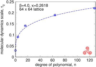
Figure 2: The characteristic time-scale $\tau_{0}$ vs polynomial degree, $N$. The dashed line guides the eye.

For low values of $N$ (the polynomial degree) the computational bottleneck is solver performance while for larger values, the evaluation of the force term arising from interactions between the gauge fields and the guide bosons begins to dominate. Effective and simple strategies for tuning the algorithm are still under investigation. We are also investigating alternative choices of polynomial filters beyond Chebyshev approximation.

MP is grateful to Enterprise-Ireland for support under grant SC/01/306.

References

- [1] A. C. Irving [UKQCD], hep-lat/0208065.
- [2] B. Joo et.al. [UKQCD], hep-lat/0005023.
- [3] A. Borici, hep-lat/0208048.
- [4] A. Duncan, E. Eichten and H. Thacker, Phys. Rev. D 59 (1999) 014505.
- [5] A. Hasenfratz and F. Knechtli, hep-lat/0203010.
- [6] K. Orginos, D. Toussaint and R. L. Sugar [MILC], Phys. Rev. D 60 (1999) 054503.
- [7] C. Alexandrou et.al. Phys. Rev. D 61 (2000) 074503.
- [8] J. C. Sexton and D. H. Weingarten, Nucl. Phys. B380, 665 (1992).
- [9] M. Hasenbusch, Phys. Lett. B 519 (2001) 177.
- [10] M. Luscher, Nucl. Phys. B 418 (1994) 637.
- [11] R. Frezzotti and K. Jansen, Phys. Lett. B 402 (1997) 328.
- [12] A. Borici and P. de Forcrand, Nucl. Phys. B 454 (1995) 645.